Convexification of Charge Equilibrium within the Dendrites of Rechargeable Batteries
Abstract
The amorphous propagation of microstructures during the electrochemical charging of a battery is the main reason for the capacity decay and short circuit. The charge distribution across the micro-structure is the result of both local and global equilibrium and is non-convex problem merely due to stochastic placement of the atoms. As such, obtaining the charge equilibrium () is a critical factor, since the amount of charge determines the success rate of the bond formation for the ionic species approaching the microstructure and consequently the ultimate morphology of the electrochemical deposits. Herein we develop a computationally-affordable method for determining the charge allocation within such microstructures. The cost function and the span of the charge distribution correlates very closely with the trivial method as well as a conventional method, albeit having significantly less computational cost. The method can be used for optimization in non-convex environments, specially those of stochastic nature.
American University of Beirut, Riad ElSolh, Beirut, Lebanon 1107-2020
Bahçeşehir University, 4 Çırağan Cad, Beşiktaş, Istanbul, Turkey 34353
California Institute of Technology, 1200 E California Blvd, Pasadena, CA 91125
Keywords: Charge Equilibrium, Dendrites, Convexification, Optimization.
1 Introduction
Metallic anodes such as lithium, sodium and zinc are arguably highly attractive candidates for use in high-energy and high-power density rechargeable batteries [1, 2, 3]. In particular, lithium metal possess the lowest density and smallest ionic radius which provides a very high gravimetric energy density and possesses the highest electropositivity ( vs SHE) that likely provides the highest possible voltage, making it suitable for high-power applications such as electric vehicles. ()[4, 5]. During the charging, the fast-pace formation of microstructures with relatively low surface energy from Brownian dynamics, leads to the branched evolution with high surface to volume ratio [6]. The quickening tree-like morphologies could occupy a large volume, possibly reach the counter-electrode and short the cell (Figure 1a). Additionally, they can also dissolve from their thinner necks during subsequent discharge period. Such a formation-dissolution cycle is particularly prominent for the metal electrodes due to lack of intercalation111Intercalation: diffusion into inner layer as the housing for the charge, as opposed to depositing in the surface.[1]. Previous studies have investigated various factors on dendritic formation such as current density[7], electrode surface roughness [8, 9, 10], impurities [11], solvent and electrolyte chemical composition [12, 13], electrolyte concentration [14], utilization of powder electrodes [15] and adhesive polymers[16], temperature [17], guiding scaffolds [18, 19], capillary pressure [20], cathode morphology [21] and mechanics [22, 23]. Some of conventional characterization techniques used include NMR [24] and MRI [25]. Recent studies also have shown the necessity of stability of solid electrolyte interphase (i.e. SEI) layer for controlling the nucleation and growth of the branched medium [26, 27].
Earlier model of dendrites had focused on the electric field and space charge as the main responsible mechanism [28] while the later models focused on ionic concentration causing the diffusion limited aggregation (DLA) [29, 30, 31]. Both mechanisms are part of the electrochemical potential [32, 33], indicating that each could be dominant depending on the localizations of the electric potential or ionic concentration within the medium. Nevertheless, their interplay has been explored rarely, especially in continuum scale and realistic time intervals, matching scales of the experimental time and space.
Dendrites instigation is rooted in the non-uniformity of electrode surface morphology at the atomic scale combined with Brownian ionic motion during electrodeposition. Any asperity in the surface provides a sharp electric field that attracts the upcoming ions as a deposition sink. Indeed the closeness of a convex surface to the counter electrode, as the source of ionic release, is another contributing factor. In fact, the same mechanism is responsible for the further semi-exponential growth of dendrites in any scale. During each pulse period the ions accumulate at the dendrites tips (unfavorable) due to high electric field in convex geometry and during each subsequent rest period the ions tend to diffuse away to other less concentrated regions (favorable). The relaxation of ionic concentration during the idle period provides a useful mechanism to achieve uniform deposition and growth during the subsequent pulse interval. Such dynamics typically occurs within the double layer (or stern layer [34]) which is relatively small and comparable to the Debye length. In high charge rates, the ionic concentration is depleted and concentration on the depletion reaches zero [35]; nonetheless, our continuum-level study extends to larger scale, beyond the double layer region [36].
Various charging protocols have been utilized for the prevention of dendrites [37], which has previously been used for uniform electroplating [38]. We have proven that the optimum rest period for the suppression of dendrites correlates with the relaxation time of the double layer for the blocking electrodes which is interpreted as the RC time of the electrochemical system [39]. We have explained qualitatively how relatively longer pulse periods with identical duty cycles will lead to longer and more quickening growing dendrites [40]. We developed coarse grained computationally affordable algorithm that allowed us reach to the experimental time scale (). Additionally, in the recent theoretical work we indicated that there is an analytical criterion for the optimal inhibition of growing dendrites [41].
Additionally, the ultimate morphology of the dendritic electrodeposites, depends on the possibility of the bond-formation when ion reaches the outer boundary of the microstructure. The success of electron transfer in such approach would highly be determined to the amount of the charge presents in the electron transfer site. Therefore, in this paper, we elaborate on the charge distribution in equilibrium across the dendritic microstructures, where the placement of the stochastically-grown dendrites. Subsequently, we verify our method via comparison with trivial method, which is far more computationally expensive as well as a conventional package. The convexification of charge distribution can be utilized widely, as well as the charge equilibrium in the electrodeposits.
2 Methodology
2.1 Computational Method


Figure 1 represents the dendritic propagation in the lab scale as well as in our computations. The ionic flux is generated in response to the variation of the electrochemical potential, which is per see the result of the variations (i.e. gradient) of concentration () or electric potential (). In the ionic scale, the regions of higher concentration tend to collide and repel more and, given enough time, diffuse to lower concentration zones, following Brownian motion. Such inter-collisions could be added-up in the larger scale and be addressed via diffusion length [40] 222The diffusion coefficient is generally concentration dependent [43], due to dilute concentration in the electro-neutral region, we assume the negligible variations. representing the average progress of a diffusive wave in a given time and is obtained directly from the diffusion equation [44]. On the other hand, ions tend to acquire drift velocity in the electrolyte medium when exposed to electric field and during the given time their progress by the drift velocity.
Therefore the total effective displacement with neglecting convection333Convection-wise, since the Rayleigh number is highly dependent to the thickness (i.e. ), for a thin layer of electrodeposition we have and thus the convection is negligible. [45] would be:
| (1) |
where is the ionic diffusion coefficient in the electrolyte, is the coarse time interval444 where is the inter-collision time, typically in the range of ., is a normalized vector in random direction, representing the Brownian dynamics, is the mobility of cations in electrolyte and is the local electric field, which is the gradient of electric potential ( ). Such vector sum is represented in the Figure 1b.
The probability of successful jump depends on how much charge each atom has from the sea of electrons. Such charge equilibrium would be obtained from the minimization of the total potential energy for the amorphous material, which is generally obtained by means of Taylor expansion as [46]:
| (2) |
where the second term in Equation 2 is in fact the electronegativity and is defined by:
since all the composing atoms in dendrites are identical the variation in fact breaks down to the cost function as the difference in the total potential energy based on the charge allocation as:
| (3) |

where is the interatomic distance from to defined as:
and and are the coordinates of the atoms relative to a reference point. Assuming that the set of charge values could be represented by the vector , one can interpret the optimization problem in the quadratic form as:
| (4) |
where the total energy is in fact the matrix from of Equation 3 and the reciprocal distance matrix is stablished:
and and are the valence electrons and electron charge respectively. The first constraint in Equation 4 means that the total sum of charges is a constant value given to the dendrite and the second and third constraints determine the capacity range of charge fraction for each atom in the microstructure.
2.1.1 Locating minimum charge
The energy difference defined by Equation 4 as the cost function is depends on the charge allocation in the atoms as well as their distance. Assuming the given charge to a charge, in order to minimize the energy term , the corresponding charges with the lower distance (closer) should contain lower relative charge values and vice versa. In fact the allocation of charges should be such that the most populated atomic regions in the crystal, formed by the random walk procedure, should contain the lowest fraction of the charge, since the denominator in the Equation 3 is quite large in those regions. Such position in fact could be obtained for the case of even distribution in the atomic charges. Assuming as such position, the value of the reciprocal distance sum should be the maximum:
| (5) |
The minimum charge via this this expression signifies it’s the closest proximity to the other charges.

2.1.2 Convexification
Finding the closest proximity of the minimum charge in the Equation 5 ensures the closest radial distance to the surrounding atoms. In other words, the largest allocation of charge magnitude should be given to the atoms farthest from the the most compact regions. Therefore, starting from the minimum charge as the reference and moving outward radially, any charge distribution should have an increasing trend, and there will be no sensitivity for variation in the azimuthal direction as:
As well, the quadratic form of the potential energy in Equation 3 suggests that the charge distribution in the radial direction has convex shape, which we translate in the radial direction to:
Performing numerical segmentation, this typically leads to for consecutive charges. Since the atoms possess non-uniform spacing, we arrive at:
noting the difference in the slope we arrive the following:
therefore the value of charge consecutively can be obtained as:
| (6) |
| Parameter | Symbol | Value | Unit |
|---|---|---|---|
| # atoms | |||
| Diffusivity | |||
| Permittivity | |||
| Temperature | |||
| Domain length | |||
| Voltage |
The Equation 6 assigns to a charge a value that ascribes convexity to the distribution given the charge value of preceding points. Furthermore, it establishes convexification of randomly distributed points starting from a minimum charged atom. Such iteration has been performed for multiple values of the variation difference for the charge distribution based on the constraints in the Equation 4 such that the minimum value of the objective function (Eq. 3) is obtained. The outlined algorithm has been visualized in the Figure 2 based on the parameters given in the Table 1. Figure 3 shows the charge distribution within the given stochastically-developed microstructure, where the location of the minimum charge is highlighted. The black lines and green vectors represent the iso-potential contours and electric field respectively.
2.2 Sample Computation
We carry out the sample computation for the method we have developed and we compare it against the conventional MATLAB framework, as well as the trivial solutions, and filtered trivial solution. We study the one dimensional case where atoms are allocated in a straight line based on the numbers given in the Table 2. Here we propose the following methods to compare to:
| 11 | 11 | -10 | 10 | 0 | 3.66 |
2.2.1 Analytical Solution
Since the central position from Equation 3 can be regarded as the minimum charge point, we can interpret that the center of the 1D line could be the location for the minimum charge. From the constraints in the Equation 4, the type of analytical function can be extracted. The charge should have the increasing slope condition as well as positive second derivative for the formation of the convex shape. If is the one dimensional coordinates, therefore analogous to the given constraints the forms are obtained as:
where . The line will have a symmetric charge distribution, one could study one of it’s identical halves, using the combinatorics the two forms via absorbing the two coefficients and into the new pre-factor . Considering the continuum-scale linear charge density the charge distribution would have a form of:
Therefore the energy minimization in Equation 4 will translate into the following:
| (7) |
Exact solution
Assuming: , one needs to find two free parameters , . The total energy can be obtained as:
and the constraints will be obtained using the chain derivative rule as:
Since the distribution form is increasing the boundary condition should satisfy at the end () and therefore:
Considering the maximum value in the inequality, we arrive to the following via combination:
This is a quadratic equation versus the exponent . Therefore, assuming it can be solved and the charge density is obtained as:
| (8) |
Simplified solution
The exact form of charge distribution in Equation 8 can be approximated with a simpler form. Here we prove that the exponent has an upper bound of :
Proving for maximum case one has:
| (9) |
Since the is positive value, the we must have:
As well the square sign should be non-negative, therefore:
Taking the inequality 9 to the power 2 we get:
which is always true and the upper bound is determined. Therefore the exponent could be considered as . Thus the sum condition gives:
and the coefficient is updated accordingly versus the total charge sum . Hence, the simplified charge would be:
| (10) |
Note that this is valid for and the other (negative) half can be established from symmetry.
2.2.2 Enhanced Trivial Method
Using the trivial method, we iteratively scan the charge distribution which minimizes the total energy in Equation 4 from the all possible permutations from combinatorics. The approximate iterative solution could be finding the non-zero integer distribution to the pre-determined sum constraint given as:
| (11) |
where, due to integer nature of the solution, the fixed total sum has been augmented -fold to allow higher precision of the distribution and the resulted distribution will ultimately scaled back -fold to satisfy the sum constraint in Equation 4. As well, the range constraints could been translated into the followings to save a significant portion of the trivial solutions from Equation 11:
| (12) |
The next comparison has been performed with the conventional MATLAB package function in terms of cost and accuracy. Since this function locates the local minima, it was run for different initial distribution values in the close proximity of the analytical solution, to target the global minimum. As well, the initial condition was given based on the analytical solution in the Equation 10.
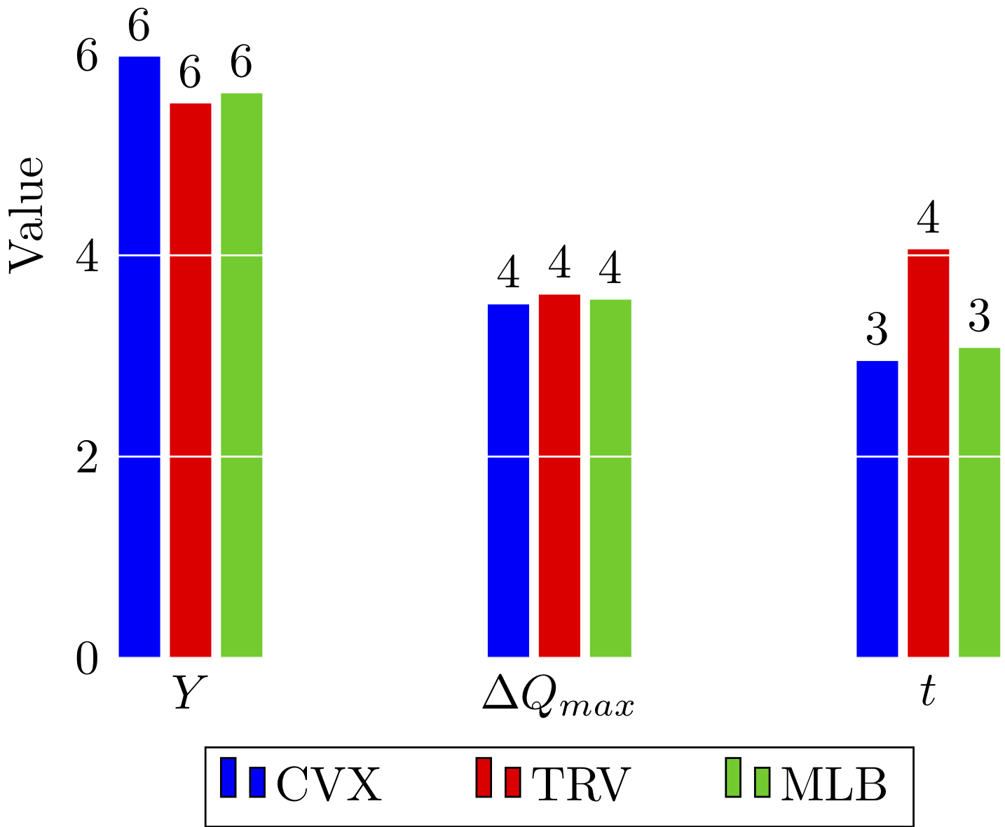
The resulted distributions have been visualized in the Figure 4a and the corresponding significant numbers are compared in the Figure 4a. It is worth noting that the computational time required for the trivial case post-filtration is significantly less than the filtered cases via Equation 12, with the factor of .

3 Results & Discussions
Finding the minimum energy for amorphous microstructures is usually a non-convex problem, which makes it difficult to solve. This is merely due to stochastic allocation of the atoms. Since the reciprocal distance matrix is symmetric (), for any given matrix there exists matrix such that:
Due to symmetry, the trace of reciprocal matrix is the sum of it’s eigenvalues . Since, the distance of each atom to itself is zero, and hence:
the zero-sum constraint shows that at least one eigenvalue is negative. Therefore the problem is not convex.
The flowchart 2 shows the information flow for determining the charge allocation leading to the minimum energy , which is mainly divided into two compartment of locating the minimum charge, and establishing a convex charge distribution. Such division in fact is an approximation, providing a significantly less computational cost versus the whole-in minimization of the total energy given in the Equation 3. In fact, the minimization of the reciprocal distance sum in the Equation 5 ensures that the most populated central (body) regions would be the location of the minimum charge and vice versa, the outer (boundary) regions would possess the highest portion of the charge sum, since they will be farthest from the rest of the atoms to create large potentials. This has been illustrated in the random dendritic microstructure illustrated in the Figure 3. Such allocation means that the outer atoms in fact will have higher possibility for the electron donation rather than the inner layers.
The comparative analysis of our method has been performed for the 1D arrangement of the atoms based on the Table 2. The verification has been illustrated versus the enhanced trivial search method as well as the commercial package. The accuracy comparison is shown in the Figure 4a and the effectiveness is represented in the Figure 4b.


Additionally the advantage of the developed method is that the result is independent of the initial condition, as opposed to the commercial package. Typical methods of finding the optimum solution requires wither restricting the search within a convex set [47], or relaxing non-convex constraints [48, 49]. Our method is numerically following the same track, searching iteratively via small perturbations in the convexity (Fig. 5a) to obtain the minimum energy . Additionally the developed method finds the optimum charge distribution via the physical and spatial awareness of the convex dispersal of the charge. Such convex hull is illustrated in the Figure 5b, where the colors qualitatively represent the relative charge values.
4 Conclusions
In this paper, we developed a convexification method for the charge equilibrium within the given stochastically-evolved dendritic microstructure. Our computationally affordable method, which has mainly been divided to simpler compartments, has been compared against the conventional method as well as the commercial packages.
The significance of the method is the independence from the initial condition and very low computational cost. Our method could be used for determining the charge allocation in a larger clusters of microstructures where the convex optimization would not be possible. In particular the charge magnitude would determine the reaction probability, the rate of propagation and the densification of microstructure during the branched evolution.
Acknowledgement
We would like to thank internal support from the Faculty of Engineering and Architecture at American University of Beirut.
References
- [1] Zhe Li, Jun Huang, Bor Yann Liaw, Viktor Metzler, and Jianbo Zhang. A review of lithium deposition in lithium-ion and lithium metal secondary batteries. J. Power Sources, 254:168–182, 2014.
- [2] Pucheng Pei, Keliang Wang, and Ze Ma. Technologies for extending zinc air batterys cyclelife: A review. Applied Energy, 128:315–324, 2014.
- [3] Michael D Slater, Donghan Kim, Eungje Lee, and Christopher S Johnson. Sodium-ion batteries. Adv. Funct. Mater., 23(8):947–958, 2013.
- [4] Siyuan Li, Jixiang Yang, and Yingying Lu. Lithium metal anode. Encyclopedia of Inorganic and Bioinorganic Chemistry, pages 1–21.
- [5] W. Xu, J. L. Wang, F. Ding, X. L. Chen, E. Nasybutin, Y. H. Zhang, and J. G. Zhang. Lithium metal anodes for rechargeable batteries. Energy and Environmental Science, 7(2):513–537, 2014.
- [6] Kang Xu. Nonaqueous liquid electrolytes for lithium-based rechargeable batteries. Chemical Reviews-Columbus, 104(10):4303–4418, 2004.
- [7] F. Orsini A.D. Pasquier B. Beaudoin J.M. Tarascon et al. In situ scanning electron microscopy (sem) observation of interfaces with plastic lithium batteries. J. Power Sources, 76:19–29, 1998.
- [8] C. Monroe and J. Newman. The effect of interfacial deformation on electrodeposition kinetics. J. Electrochem. Soc., 151(6):A880–A886, 2004.
- [9] Christoffer P Nielsen and Henrik Bruus. Morphological instability during steady electrodeposition at overlimiting currents. arXiv preprint arXiv:1505.07571, 2015.
- [10] PP Natsiavas, K Weinberg, D Rosato, and M Ortiz. Effect of prestress on the stability of electrode–electrolyte interfaces during charging in lithium batteries. Journal of the Mechanics and Physics of Solids, 95:92–111, 2016.
- [11] J. Steiger, D. Kramer, and R. Monig. Mechanisms of dendritic growth investigated by in situ light microscopy during electrodeposition and dissolution of lithium. J. Power Sources, 261:112–119, 2014.
- [12] N. Schweikert, A. Hofmann, M. Schulz, M. Scheuermann, S. T. Boles, T. Hanemann, H. Hahn, and S. Indris. Suppressed lithium dendrite growth in lithium batteries using ionic liquid electrolytes: Investigation by electrochemical impedance spectroscopy, scanning electron microscopy, and in situ li-7 nuclear magnetic resonance spectroscopy. J. Power Sources, 228:237–243, 2013.
- [13] Reza Younesi, Gabriel M Veith, Patrik Johansson, Kristina Edström, and Tejs Vegge. Lithium salts for advanced lithium batteries: Li-metal, li-o 2, and li-s. Energy and Environmental Science, 8(7):1905–1922, 2015.
- [14] C. Brissot, M. Rosso, J. N. Chazalviel, and S. Lascaud. In situ concentration cartography in the neighborhood of dendrites growing in lithium/polymer-electrolyte/lithium cells. J. Electrochem. Soc., 146(12):4393–4400, 1999.
- [15] I. W. Seong, C. H. Hong, B. K. Kim, and W. Y. Yoon. The effects of current density and amount of discharge on dendrite formation in the lithium powder anode electrode. J. Power Sources, 178(2):769–773, 2008.
- [16] GM Stone, SA Mullin, AA Teran, DT Hallinan, AM Minor, A Hexemer, and NP Balsara. Resolution of the modulus versus adhesion dilemma in solid polymer electrolytes for rechargeable lithium metal batteries. J. Electrochem. Soc., 159(3):A222–A227, 2012.
- [17] Asghar Aryanfar, Tao Cheng, Agustin J Colussi, Boris V Merinov, William A Goddard III, and Michael R Hoffmann. Annealing kinetics of electrodeposited lithium dendrites. The Journal of chemical physics, 143(13):134701, 2015.
- [18] Yuanzhou Yao, Xiaohui Zhao, Amir A Razzaq, Yuting Gu, Xietao Yuan, Rahim Shah, Yuebin Lian, Jinxuan Lei, Qiaoqiao Mu, Yong Ma, et al. Mosaic rgo layer on lithium metal anodes for effective mediation of lithium plating and stripping. Journal of Materials Chemistry A, 2019.
- [19] Ji Qian, Yu Li, Menglu Zhang, Rui Luo, Fujie Wang, Yusheng Ye, Yi Xing, Wanlong Li, Wenjie Qu, Lili Wang, et al. Protecting lithium/sodium metal anode with metal-organic framework based compact and robust shield. Nano Energy, 2019.
- [20] Wei Deng, Wenhua Zhu, Xufeng Zhou, Fei Zhao, and Zhaoping Liu. Regulating capillary pressure to achieve ultralow areal mass loading metallic lithium anodes. Energy Storage Materials, 2019.
- [21] Alexander W Abboud, Eric J Dufek, and Boryann Liaw. Implications of local current density variations on lithium plating affected by cathode particle size. Journal of The Electrochemical Society, 166(4):A667–A669, 2019.
- [22] Chen Xu, Zeeshan Ahmad, Asghar Aryanfar, Venkatasubramanian Viswanathan, and Julia R Greer. Enhanced strength and temperature dependence of mechanical properties of li at small scales and its implications for li metal anodes. Proceedings of the National Academy of Sciences, 114(1):57–61, 2017.
- [23] Peng Wang, Wenjie Qu, Wei-Li Song, Haosen Chen, Renjie Chen, and Daining Fang. Electro–chemo–mechanical issues at the interfaces in solid-state lithium metal batteries. Advanced Functional Materials, page 1900950, 2019.
- [24] Rangeet Bhattacharyya, Baris Key, Hailong Chen, Adam S Best, Anthony F Hollenkamp, and Clare P Grey. In situ nmr observation of the formation of metallic lithium microstructures in lithium batteries. Nat. Mater., 9(6):504, 2010.
- [25] S Chandrashekar, Nicole M Trease, Hee Jung Chang, Lin-Shu Du, Clare P Grey, and Alexej Jerschow. 7li mri of li batteries reveals location of microstructural lithium. Nat. Mater., 11(4):311–315, 2012.
- [26] Yunsong Li and Yue Qi. Energy landscape of the charge transfer reaction at the complex li/sei/electrolyte interface. Energy & Environmental Science, 2019.
- [27] Laleh Majari Kasmaee, Asghar Aryanfar, Zarui Chikneyan, Michael R Hoffmann, and AgustÃn J Colussi. Lithium batteries: Improving solid-electrolyte interphases via underpotential solvent electropolymerization. Chem. Phys. Lett., 661:65–69, 2016.
- [28] J. N. Chazalviel. Electrochemical aspects of the generation of ramified metallic electrodeposits. Phys. Rev. A, 42(12):7355–7367, 1990.
- [29] C. Monroe and J. Newman. Dendrite growth in lithium/polymer systems - a propagation model for liquid electrolytes under galvanostatic conditions. J. Electrochem. Soc., 150(10):A1377–A1384, 2003.
- [30] Thomas A Witten and Leonard M Sander. Diffusion-limited aggregation. Phys. Rev. B, 27(9):5686, 1983.
- [31] Xin Zhang, Q Jane Wang, Katharine L Harrison, Katherine Jungjohann, Brad L Boyce, Scott A Roberts, Peter M Attia, and Stephen J Harris. Rethinking how external pressure can suppress dendrites in lithium metal batteries. Journal of The Electrochemical Society, 166(15):A3639–A3652, 2019.
- [32] Allen J. Bard and Larry R. Faulkner. Electrochemical methods: fundamentals and applications. 2 New York: Wiley, 1980., 1980.
- [33] Deepti Tewari and Partha P Mukherjee. Mechanistic understanding of electrochemical plating and stripping of metal electrodes. Journal of Materials Chemistry A, 7(9):4668–4688, 2019.
- [34] Martin Z Bazant, Brian D Storey, and Alexei A Kornyshev. Double layer in ionic liquids: Overscreening versus crowding. Phys. Rev. Lett., 106(4):046102, 2011.
- [35] V. Fleury. Branched fractal patterns in non-equilibrium electrochemical deposition from oscillatory nucleation and growth. Nature, 390(6656):145–148, 1997.
- [36] Asghar Aryanfar, Daniel J Brooks, AgustÃn J Colussi, Boris V Merinov, William A Goddard III, and Michael R Hoffmann. Thermal relaxation of lithium dendrites. Phys. Chem. Chem. Phys., 17(12):8000–8005, 2015.
- [37] Jun Li, Edward Murphy, Jack Winnick, and Paul A Kohl. The effects of pulse charging on cycling characteristics of commercial lithium-ion batteries. J. Power Sources, 102(1):302–309, 2001.
- [38] M. S. Chandrasekar and M. Pushpavanam. Pulse and pulse reverse plating - conceptual, advantages and applications. Electrochim. Acta, 53(8):3313–3322, 2008.
- [39] M. Z. Bazant, K. Thornton, and A. Ajdari. Diffuse-charge dynamics in electrochemical systems. Physical Review E, 70(2), 2004.
- [40] Asghar Aryanfar, Daniel Brooks, Boris V. Merinov, William A. Goddard Iii, AgustÃn J. Colussi, and Michael R. Hoffmann. Dynamics of lithium dendrite growth and inhibition: Pulse charging experiments and monte carlo calculations. The Journal of Physical Chemistry Letters, 5(10):1721–1726, 2014.
- [41] Asghar Aryanfar, Daniel J Brooks, and William A Goddard. Theoretical pulse charge for the optimal inhibition of growing dendrites. MRS Advances, 3(22):1201–1207, 2018.
- [42] Asghar Aryanfar, Michael R Hoffmann, and William A Goddard III. Finite-pulse waves for efficient suppression of evolving mesoscale dendrites in rechargeable batteries. Physical Review E, 100(4):042801, 2019.
- [43] S Chandrashekar, Onyekachi Oparaji, Guang Yang, and Daniel Hallinan. Communication 7li mri unveils concentration dependent diffusion in polymer electrolyte batteries. Journal of The Electrochemical Society, 163(14):A2988–A2990, 2016.
- [44] Jean Philibert. One and a half century of diffusion: Fick, einstein, before and beyond. Diffusion Fundamentals, 4(6):1–19, 2006.
- [45] Philip J Pritchard, John W Mitchell, and John C Leylegian. Fox and McDonald’s Introduction to Fluid Mechanics, Binder Ready Version. John Wiley & Sons, 2016.
- [46] Anthony K Rappe and William A Goddard III. Charge equilibration for molecular dynamics simulations. The Journal of Physical Chemistry, 95(8):3358–3363, 1991.
- [47] Behçet Açıkmeşe, John M Carson, and Lars Blackmore. Lossless convexification of nonconvex control bound and pointing constraints of the soft landing optimal control problem. IEEE Transactions on Control Systems Technology, 21(6):2104–2113, 2013.
- [48] Changliu Liu, Chung-Yen Lin, Yizhou Wang, and Masayoshi Tomizuka. Convex feasible set algorithm for constrained trajectory smoothing. In 2017 American Control Conference (ACC), pages 4177–4182. IEEE, 2017.
- [49] Changliu Liu, Chung-Yen Lin, and Masayoshi Tomizuka. The convex feasible set algorithm for real time optimization in motion planning. SIAM Journal on Control and optimization, 56(4):2712–2733, 2018.