Convergence estimates for the Magnus expansion IIA. matrices with operator norm
Abstract.
We review and provide simplified proofs related to the Magnus expansion, and improve convergence estimates. Observations and improvements concerning the Baker–Campbell–Hausdorff expansion are also made.
In this Part IIA, we investigate the case of matrices with respect to the operator norm. We consider norm estimates and minimal presentations in terms of the Magnus and BCH expansions. Some results are obtained in the complex case, but a more complete picture is obtained in the real case.
Key words and phrases:
Magnus expansion, Baker–Campbell–Hausdorff expansion, growth estimates, Davis–Wielandt shell, conformal range of operators, minimal exponential presentations2010 Mathematics Subject Classification:
Primary: 47A12, 15A16, Secondary: 15A60.Introduction to Part IIA
The present paper is a direct continuation of Part II [12]. This assumes general familiarity with Part I [11] and a good understanding of Part II [12]. In Part II, we obtained norm estimates and inclusion theorems with respect to the conformal range. In Part IIA, we take a closer look to the more treatable case of matrices. Some investigations will be about testing or sharpening our earlier results for matrices; other ones will deal with minimal Magnus or Baker–Campbell–Hausdorff presentations. Studying matrices may seem to be a modest objective, but, in reality, the computations are not trivial. (Basic analytical calculations already appear in Magnus [15]; and more sophisticated techniques appear in Michel [16] but in the context of the Frobenius norm. Our computations are similar in spirit but more complicated, as the operator norm is taken seriously.) The information exhibited here is relatively more complete in the case of real matrices, and much more partial in the case of complex matrices.
In Section 1, we recall some theorems and examples from Part II. Our results here with respect to matrices can be viewed relative to these. In Section 2, we review some technical tools concerning matrices. To a variable extent, all later sections use the information discussed here, hence the content of this section is crucial (despite its elementary nature); however, its content can be consulted as needed later. Nevertheless, a cursory reading is advised in any case.
Section 3 and 4 discuss how Schur’s formulae and the BCH formula simplify for matrices, respectively. In Section 5, we show that for complex matrices exponentials only rarely play the “role of geodesics” (i. e. parts of minimal Magnus presentations). In Section 6, examples of BCH expansions from are given with interest in norm growth. In Section 7, we demonstrate that (appropriately) balanced BCH expansions of real matrices with cumulative norm are uniformly bounded. Next, we turn toward BCH minimal presentations of real matrices (with norm restrictions). Sections 8 and 9 study the moments of the Schur maps and apply them to minimal BCH presentations. In Section 10, the (critical) “BCH unit ball” is described resulting the “wedge cap”. At this point several further questions are left open, but having that prime interesting case seen, we leave the discussion of BCH presentations here.
Then, we start the investigation of Magnus (minimal) expansions for real matrices. We find that, in this setting, Magnus minimal presentations are more natural and approachable than BCH minimal presentations. In Section 11, we prove a logarithmic monotonicity property for the principal disks of real matrices. In Section 12 we consider some examples which test our earlier norm estimates for the Magnus expansion but also help to understand the real case better by introducing the “canonical Magnus developments”. Section 13 develops a systematic analysis of the real case. The first observation is that in this case the Magnus exponent can be read off from the conformal range / principal disk. Based on the previous examples, we consider (minimal) normal presentations for real matrices given as time-ordered exponentials which are not ordinary exponentials. The conclusion is that those normal presentations are better suited to the geometric description of than the customary exponentials. In Section 14, we give information about the asymptotics of the optimal norm estimate for real matrices. In Section 15, however, it is demonstrated that the Magnus exponent of complex matrices cannot be read off from the conformal range as simply as in the real case. (Thus the previous methods cannot transfer that easily.)
Notation and terminology
Line of formula will be denoted as . If are points of an Euclidean (or just affine) space, then denotes the segment connecting them. This notation is also applied for (half-)open segments. It can also be used in conveniently when . Instead of ‘by the unicity principle of analytic continuation’ we will often say ‘by analytic continuation’ even if the function is already constructed. In general, we try to follow the notations established in Parts I and II.
1. Some results from Part II (Review)
Here we recall some points of Part II.
It cannot replace the detailed discussion given in Part II, but it serves reference.
1.A. Conformal range
Suppose that is a real Hilbert space. The logarithmic distance on is given by
| (1) |
Theorem 1.1.
Suppose that is continuous. Then
In case of equality, is a (not necessarily strictly) monotone subpath of a distance segment connecting to . ∎
For let be denote their angle. This can already be obtained from the underlying real scalar product . For , , let
For , we define the (extended) conformal range as
and the restricted conformal range as
(This is a partial aspect of the Davis-Wielandt shell, see Wielandt [20], Davis [5], [6] and also [12].)
Theorem 1.2.
(Time ordered exponential mapping theorem.)
If is -valued ordered measure, then
| (2) |
and
| (3) |
In particular, if , then is well-defined, and for its spectral radius
| (4) |
1.B. Convergence theorems
Theorem 1.3.
(Mityagin–Moan–Niesen–Casas logarithmic convergence theorem.)
If is a -valued ordered measure and , then the Magnus expansion is absolute convergent. In fact, also holds.
The statement also holds if is replaced by any -algebra.
We say that the ordered measure is a multiple Baker–Campbell–Hausdorff (mBCH) measure, if, up to reparametrization, is of form . In this case, also allows a mass-normalized version
| (5) |
where , and thus . It is constructed by replacing with if , and eliminating the term if . As it is obtained by a kind a reparametrization, its Magnus expansion is not affected.
Theorem 1.4.
(Finite dimensional critical BCH convergence theorem.)
Let be a finite dimensional Hilbert space . Consider the valued mBCH measure with cumulative norm . Then, the convergence radius of the Magnus (mBCH) expansion of is greater than . In particular, finite dimensional mBCH expansions with cumulative norm converge. ∎
Lemma 1.5.
Let be a mass-normalized mBCH-measure as in (5), .
Consider all the Hilbert subspaces of such that
(i) is an invariant orthogonal decomposition for all .
(ii) , and these are orthogonal (unitary).
Then there is a single maximal such . ∎
In the context of the previous lemma, if the maximal such is , then we call reduced. In particular, this applies if .
Theorem 1.6.
(Finite dimensional logarithmic critical BCH convergence theorem.)
Let be a finite dimensional Hilbert space. Consider the valued mass-normalized mBCH measure as in (5) with cumulative norm . We claim:
(a) Unless the component operators have a common eigenvector for or (complex case), or a common eigenblock (real case), then also holds.
(b) If is reduced, then, for any , holds. Thus, the -able radius of the Magnus (BCH) expansion is also greater than . ∎
1.C. Growth estimates
For , let us define as the solution of the equation
Then is a decreasing diffeomorphism. In particular,
Theorem 1.7.
Let , . Then
| (6) |
Theorem 1.8.
(a) As ,
| (7) |
(b) As ,
| (8) |
where
(the integrand extends to a smooth function of ). Numerically, ∎
The function is not very particular, it can be improved. An example we have considered to test the effectivity of (6)–(8) was
Example 1.9.
(The analytical expansion of the Magnus critical case.)
On the interval , we consider the measure , such that
Thus, for ,
Then,
Consequently,
| (9) |
as . ∎
2. Computational background for matrices
For the sake of reference, here we review some facts and conventions
related to matrices we have already considered in Part II.
However, we also take the opportunity to augment this review
by further observations of analytical nature.
2.A. The skew-quaternionic form (review)
One can write the matrix in skew-quaternionic form
| (10) |
Then,
and
2.B. Spectral type (review)
Let us use the notation
It is essentially the discriminant of , as the eigenvalues of are .
In form (10),
| (11) |
In the special case of real matrices, we use the classification
elliptic case: two conjugate strictly complex eigenvalues,
parabolic case: two equal real eigenvalues,
hyperbolic case: two distinct real eigenvalues.
Then, for real matrices, measures ‘ellipticity/parabolicity/hiperbolicity’: If , then is elliptic; if , then is parabolic; if , then is hyperbolic.
In the general complex case, there are two main categories: parabolic and non-parabolic .
2.C. Principal and chiral disks (review)
For real matrices we can refine the spectral data as follows: Assume that . Its principal disk is
This is refined further by the chiral disk
The additional data in the chiral disk is the chirality, which is the sign of the twisted trace, This chirality is, in fact, understood with respect to a fixed orientation of . It does not change if we conjugate by a rotation, but it changes sign if we conjugate by a reflection. From the properties of the twisted trace, it is also easy too see that respects chirality.
One can read off many data from the disks. For example, if , then . This is not surprising in the light of
Lemma 2.1.
makes a bijective correspondence between possibly degenerated disks in and the orbits of with respect to conjugacy by special orthogonal matrices (i. e. rotations).
makes a bijective correspondence between possibly degenerated disks with center in and the orbits of with respect to conjugacy by orthogonal matrices. ∎
The principal / chiral disk is a point if has the effect of a complex multiplication (that is a quasicomplex matrix). In general, matrices fall into three categories: elliptic, parabolic, hyperbolic; such that the principal /chiral disk are disjoint, tangent or secant to the real axis, respectively.
2.D. Conformal range of real matrices (review)
The principal / conformal disks turn out to be closely related to the conformal range:
Lemma 2.2.
Consider the real matrix We claim:
(a) For acting on ,
(b) For acting on ,
This is but with the components of disjoint from filled in. ∎
Thus is the boundary of the principal (or chiral) disk factored by conjugation. In terms of hyperbolic geometry (in the Poincaré half-space), may yield points or circles in the elliptic case; asymptotic points or corresponding horocycles (paracycles) in the parabolic case; lines or pairs of distance lines (hypercycles) in the hyperbolic case. (In the normal case, it yields points, asymptotic points or lines; in the non-normal case, it yields circles, asymptotically closed horocycles, asymptotically closed pairs of distance lines.) is but the -convex closure.
2.E. Recognizing log-ability
For finite matrices . Consequently, is -able if and only if . ( can be replaced by ). Or, for real matrices, in terms of the principal disk, is -able if and only if . ( can be replaced by .)
2.F. Canonical forms of matrices in skew-quaternionic form
In , the effect of conjugation by a rotation matrix is given by
| (12) |
Thus, through conjugation by a rotation matrix, any real matrix can be brought into shape
with
If we also allow conjugation by , then
can be achieved. ( is the chirality class of the matrix.)
In , using conjugation by rotation matrices, the coefficient of can be eliminated. Then using conjugation by diagonal unitary matrices, the phase of the coefficient of can be adjusted. In that way the form
| (13) |
with
| , , , |
can be achieved. Conjugating by , or a similar restriction can be assumed. Using the definite abuse of notation , we find and ; and is unitary. Thus, by a further unitary conjugation,
or a similar restriction can be assumed. (We could also base a canonical form on and , but the present form is conveniently close to the real case.)
Here normal matrices are characterized by that or .
2.G. The visualization of certain subsets of
In what follows we will consider certain subsets of . By the rotational effect (12), an invariant subset is best to be visualized through the image of the mapping
( can be considered as a subset of the asymptotically closed Poincaré half-space.)
In particular, the image of the centered sphere in of radius is
a “conical hat”.
2.H. Arithmetic consequences of dimension
For complex matrices , the Cayley–Hamilton equation reads as
| (14) |
Obvious consequences are as follows: For the trace,
i. e.,
in the invertible case,
and, more generally, for the adjugate
| (15) |
Applying (15) to the identity , and expanded, we obtain
| (16) |
Lemma 2.3.
(o) Any non-commutative (real) polynomial of can be written as linear combinations of
| (18) |
with coefficients which are (real) polynomials of
| (19) | , , , , . |
(a) Any scalar expression built up from and , , using algebra operations can by written as a polynomial of (19).
(b) Any matrix expression built up from and , , using algebra operations can by written as linear combination of (18) with coefficients which are polynomials of (19).
Proof.
(o) Using (14) and (17), and also their version with the role of and interchanged, repeatedly, we arrive to linear combinations (with appropriate coefficients). Due to, (16), however, the last two terms can be traded to . (a–b) are best to be proven by simultaneous induction on the complexity of the algebraic expressions. In view of (o), the only nontrivial step is when we take determinant of a matrix expression. This, however, can be resolved by using . ∎
If we examine the proof of Lemma 2.3, we see that it also gives an algorithm for the reduction to standard form.
Example 2.4.
In general, if we allow adjoints in our expressions, then their complexity increases. We only note the identity
| (20) |
which can be checked by direct computation. (Matrix expressions with “more than two variables” can also be dealt systematically, but the picture is more complicated.)
Rearranging (14) into a full square, we obtain
| (21) |
It is useful to introduce the notation
Indeed, in (22), can be replaced by , in which form, (21) implies (22). Then (24) follows by interchange of variables, and (23) follows by polarization in the first two commutator variables.
The commutator analogue of Lemma 2.3 is
Lemma 2.5.
Any (real) commutator polynomial of with no uncommmutatored terms can be written as linear combinations of
| (25) |
with coefficients which are (real) polynomials of
| (26) | , , . |
Proof.
Commutator expressions can be reduced to linear combinations of iterated left commutators, whose ends of length four are either trivial or can be reduced by (22) or (23) (essentially). After the reduction only commutators of length or are left with appropriate coefficients. Conversely, by (22) or (23) or (24), the multipliers , , can be absorbed to commutators. ∎
Lemma 2.6.
We find:
Proof.
(a) Even the particular case of Example 2.4 demonstrates that the entries of (18) and (19) are algebraically independent over the reals. This also implies independence in general case over the reals. As all the algebraic rules are inherently real, this also implies independence over the complex numbers.
(b) It is easy to see that in the statement of Lemma 2.3, , , can be replaced by , , , respectively. Regarding the base terms, the identities
| (27) |
and
| (28) |
show the independence of the new base terms as . ∎
As a consequence, we have obtained a normal form for (formal) commutator expressions in the case of matrices. As the absorption rules (22–24) are quite simple, this normal form is quite practical.
We also mention the identities
| (29) |
| (30) |
| (31) |
which are easy to check by direct computation.
2.I. Self-adjointness, conform-unitarity, normality
Note that if is a complex self-adjoint matrix, then it is of real hyperbolic or parabolic type. Thus
with equality if and only if is a (real) scalar matrix.
In particular, for any complex matrix ,
Equality holds if and only is normal and its eigenvalues have equal absolute values, i. e. is conformal-unitary (i. e. it is a unitary matrix times a positive scalar) or is the matrix. (This follows by considering the unitary-conjugated triangular form of the matrices.) Note that the matrix is excluded from being conform-unitary. In the real case, we can speak about conform-orthogonal matrices. Then, conform-orthogonal matrices are either conform-rotations or conform-reflections.
For complex matrices, in terms of the Frobenius norm,
Thus, , , are all equivalent to the normality of . Actually, one can see, in terms of the operator norm, .
A somewhat strange quantity is . One can check that it vanishes if and only if or is conform-unitary.
Lemma 2.7.
If is a complex matrix, then
Proof.
Straightforward computation. ∎
In the case of real matrices the computations are typically much simpler, especially in skew-quaternionic form. For example,
Lemma 2.8.
If is a real matrix, then
Proof.
Simple computation. ∎
2.J. Exponentials (review, alternative)
Recall that and are entire functions on the complex plane such that
For ,
Lemma 2.9.
Let be a complex matrix. Then
Proof.
gives a decomposition to commuting operators for which, by multiplicativity, the exponential can be computed separately. In the case of the first summand this is trivial. In the case of the second summand, the identity (21) and the comparison of the power series implies the statement. ∎
2.K. The differential calculus of and (review)
First of all, it is useful to notice that
(as entire analytic functions). Then one can easily see that
and
(as entire analytic functions).
In particular, differentiation will not lead out of the rational field
generated by and .
2.L. A notable differential equation (review)
Lemma 2.10.
The solution of the ordinary differential equation
with initial data
is given by
where
In particular,
We will also use the special notation
2.M. The calculus of
In what follows, we also use the meromorphic function
has poles at , where is a positive integer. It is easy to see that
Consequently, is a differential field (induced from, say, ), which is subset of the differential field . It is not much smaller: As
it is not hard to show that the degree of the field extension is
2.N. A collection of auxiliary functions
Lemma 2.11.
The expressions
(a)
(b)
(c)
(d)
(e)
(f)
(g)
define meromorphic functions on the complex plane such that
(i) They are holomorphic on except at where is a positive integer. In those latter points they have poles of order
(ii) They are strictly monotone increasing on the interval with range .
(iii) In particular, they are strictly positive on the interval .
Proof.
These facts can be derived using various methods of (complex) analysis. ∎
The following table contains easily recoverable information:
Furthermore, it is also easy to check that the identities
hold.
Lemma 2.12.
(a) The function extends to an analytic function on (a neighbourhood of) . Special values are , .
(b) The function extends to an analytic function on (a neighbourhood of) . Special values are , .
(c) As analytic functions,
In particular, and are strictly decreasing.
Proof.
(a) It is sufficient to find a compatible extension to . One can check that, on the real line, has poles with asymptotics at for positive integers ; and otherwise is positive on the real line. This implies that
defines an appropriate extension. The special values are straightforward.
(b) As has only simple poles with asymptotics , these are cancelled out once multiplied by . The special values are straightforward.
(c) This is straightforward. ∎
2.O. The function (review, alternative)
If , and , then it is easy to see that is invertible. (For a fixed , the possible values yield the segment .) Then one can define, for ,
| (32) |
This gives an analytic function in .
Lemma 2.13.
(a) In terms of the real domain,
Note, this can be rewritten as for .
(b) As an analytic function,
| (33) |
(c) vanishes nowhere on . holds only for with .
(d) at .
(e) is strictly monotone decreasing on with range .
Proof.
(b) For , differentiating under the integral sign, we find
(a) The special value is trivial. Restricted to , using (33), we find . Considering the primitive functions, we find for , with an appropriate . As limits to a finite value for , only the case is possible. Restriction to is similar.
(e) is immediate from (32).
(c) From (32), is immediate. Then it is sufficient to restrict to . Then the statement follows from (d).
(d) Elementary analysis. ∎
From Lemma 2.13(a), it is easy to the see that, for ,
| (34) |
holds. By analytic continuation, it also holds in an open neighbourhood of .
2.P. Logarithm (review, alternative)
Recall that, in a Banach algebra, is -able if and only if the spectrum of is disjoint from . In that case, the logarithm of is defined as
| (35) |
Lemma 2.14.
Let be a real matrix.
(a) Then is a -able if and only if and .
(b) In the -able case
| (36) |
Suppose that is complex matrix which is -able. Let
One can see that this is the product of the square root of eigenvalues (with multiplicity).
Lemma 2.15.
Suppose that is complex matrix which is -able.
(a) Then , .
(b) Furthermore, the extended form of (36) holds:
| (37) |
Proofs.
Lemma 2.14(a) and Lemma 2.15(a) can be obtained from the examination of the eigenvalues in a relatively straightforward manner. For the rest, it is sufficient to prove 2.15(b). The proof is almost “tautological”: Using the differentiation rule (33), by a long but straightforward symbolic computation, one obtains, for ,
(Indeed, the symbolic computation is perfectly valid for, say, , , where ; and even can be replaced by . Then, by analyticity in and analyticity in , the general identity valid.) Integrated, (37) is obtained. ∎
2.Q. near , some asymptotics
From Lemma 2.13(a) (and analytic continuation), it easy to see that
is valid for . This is informative regarding what kind of analytic reparametrizations are useful for near . More in terms of real analysis, one has
Lemma 2.16.
(a) For , the function
is monotone decreasing with range .
(b) In particular, for ,
Proof.
Part (a) can addressed by elementary analyis. Part (a) implies part (b). ∎
2.R. Norms (review)
Lemma 2.17.
Let be a real or complex matrix. Then, for the norm,
| (38) | ||||
and, for the co-norm,
| (39) | ||||
In particular,
| (40) |
In the case of real matrices, the results are the same for the Hilbert spaces and . ∎
For matrices, we define the signed co-norm as
| (41) |
Then,
| (42) |
and
| (43) |
However, we will essentially consider the signed co-norm only for real matrices.
Lemma 2.18.
Let be a real matrix. Then
| (44) | ||||
| (45) |
On the other hand,
| (46) | ||||
It is true that
| (47) | ||||
Furthermore,
| (48) | ||||
2.S. Directional derivatives
Whenever is a function on an open domain of matrices, we define the derivative of at in direction , along smooth curves as
whenever it gives the same value for all such that is smooth, , . This is a sufficiently flexible notion to deal with some mildly singular . If is smooth, then the directional derivatives agrees to the usual multidimensional differential. E. g.
or
| (49) |
| (50) |
| (51) |
Furthermore,
| (54) |
2.T. Smoothness of norm
Now we examine the smoothness properties of the norm of complex matrices. For a complex matrix , we set
(This is the higher eigenvalue of .) It is easy to see that for
(complex coefficients), it yields
Lemma 2.19.
(o) On the space of complex matrices, the norm operation is smooth except at matrices such that the “norm discriminant”
(a) The directional derivative of the function at , along smooth curves, is, just
(b) The directional derivative of the function at , along smooth curves, is
(c) The directional derivative of the function at any conform-unitary , along smooth curves, is
(d) The directional derivative of the function at any not conform-unitary , is
Proof.
(o) The smoothness part follows from the norm expressions (38/1–2). The non-smoothness part will follow from the explicit expressions for the directional derivatives. Part (a) is trivial. Part (b) is best to be done using Taylor expansions of smooth curves. Part (c) follows from (b) by the conform-unitary displacement argument: Neighbourhoods of conform-unitary matrices are related to each other just by multiplication by conform-unitary matrices (left or right, alike). Such a multiplication, however, just simply scales up the norm. Part (d) follows from the basic observations (49–51) and standard composition rules. ∎
Remark 2.20.
For the sake of curiosity, we include the corresponding statement for co-norms. Here the situation is analogous but slightly more complicated as there is an additional case for non-smoothness. Indeed, the signed co-norm (41) has similar smoothness properties as the norm. However, when absolute value is taken to obtain the co-norm, then there is an additional source for non-smoothness: the case when the determinant vanishes.
For a complex matrix , we set
(This is the lower eigenvalue of .) It is easy to see that for
(complex coefficients), it yields
Lemma 2.21.
(o) On the space of complex matrices, the co-norm operation is smooth except at matrices such that
or
(a) The directional derivative of the function at , along smooth curves, is, just
(á) The directional derivative of the function at with , , along smooth curves, is
(In this case, and .)
(b) The directional derivative of the function at , along smooth curves, is
(c) The directional derivative of the function at any conform-unitary , along smooth curves, is
(In this case, .)
(d) The directional derivative of the function at any not conform-unitary , is
Proof.
Similar to the previous statement. ∎
For the signed co-norm, the corresponding statement to Lemma 2.19 is easy to recover from
(for ). But this counterpart to Lemma 2.19 is not particularly simple.
However, things are manageable for real matrices; which case is even more simple as the use of and can be avoided:
Lemma 2.22.
(o) On the space of real matrices, the norm and signed co-norm operations are smooth except at matrices such that
(a) The directional derivative of the function at , along smooth curves, is
The directional derivative of the function at , along smooth curves, is
(b) The directional derivative of the function at , along smooth curves, is
Here, for (with real coefficients),
The directional derivative of the function at , along smooth curves, is
Here, for (with real coefficients),
(c) The directional derivative of the function at any conform-unitary , along smooth curves, is
The directional derivative of the function at any conform-unitary , along smooth curves, is
(In this case, .)
(d) The directional derivative of the function at any not conform-unitary , is
The directional derivative of the function at any not conform-unitary , is
Proof.
It follows from the complex picture. ∎
Next, we concentrate on a special case regarding complex matrices.
Lemma 2.23.
(a) Let be a complex matrix. Then
(b) With some abuse of notation, for , let
Then,
and
(c) The map
is smooth, with the possible exception of . However, if is non-normal (or ), then smoothness also holds at .
Proof.
(a), (b) are straightforward computations. This follows from (a), (b) and the concrete form of the norm. Note that the vanishing of is equivalent to normality. ∎
Lemma 2.24.
Suppose that is a complex matrix.
(a) If is conform-orthogonal, then
(b) In the generic case ,
(c) Consequently, if , then
(d) Consequently, if is normal, then
2.U. Some inequalities for norms
Corollary 2.25.
(a) If is a real matrix, then
and
The inequalities are strict if .
(b) In fact, if , then the maps
and
are strictly decreasing on the interval .
Proof.
(a) If is written as in (10), then the inequalities trivialize as and .
(b) follows along similar lines. ∎
Corollary 2.26.
(a) If is a complex matrix, then
The inequality is strict if .
(b) In fact, if , then the map
is strictly decreasing on the interval .
Proof.
It is sufficient to prove (b), which follows from Lemma 2.24(c). ∎
(Similar statement is not true for the unsigned co-norm, not even in the real case.)
2.V. Moments of linear maps
If is a (real) linear map, then it can be represented uniquely by a complex matrix such that
This matrix is the moment associated to .
2.W. Possible exponentials from (review)
Lemma 2.28.
For , let us consider the set
The the following hold:
(a) If is hyperbolic () with two positive eigenvalues,
where is hyperbolic, with .
(b) If is hyperbolic () with no two positive eigenvalues, then
(c) If is a positive scalar matrix, then
Among its elements, the one with the lowest norm is .
(d) If is a negative scalar matrix, then
Among its elements, the two elements with the lowest norm are and . ( is not log-able).
(e) If is parabolic () but not a positive or negative scalar matrix, then
(f) If is elliptic (), then there are unique and and such that and
In that case,
Among its elements, the one with the lowest norm is .
Proof.
can be recovered by elementary linear algebra. The comments about the norms follow from the simple norm expression of (44/3). (Note that the skew-involutions are all traceless.) ∎
2.X. Further particularities in the real case
(I) If is a real matrix, then we set
This operation is chiral; if is orthogonal, then . One can check that
(Other reasonable choice would be .)
(II) Assume that is a real matrix such that . We define the -distortion (multiplicative distortion) of as
2.Y. The flattened hyperboloid model HP and some relatives
(Recall, a review of hyperbolic geometry can be found in Berger [2]; for our conventions, see [12].)
The flattened hyperboloid model, sometimes also popularized as the “Gans model” (cf. [7]), is the “vertical” projection of the usual hyperboloid model. The transcription from the CKB model is
and the transcription to the CKB model is
An advantage of HP is that its points are represented by points of ; its disadvantage is, however, that the asymptotical points of the hyperbolic plane are represented only by asymptotical points of .
For technical reasons, we will also consider the -transformed HP model with
The problem with construction is that it not well-adapted to asymptotic points, except at , where it (or, rather, its inverse) realizes blow-ups.
For this reason, a similar but better construction can be derived from the CKB model, we let
It (or, rather, its inverse) realizes a blow-up of unit disk of CKB with to . The points are blown up.
3. Schur’s formulae for matrices
3.A. BCH and Schur’s formulae (review)
Recall, that for formal variables and ,
| (55) |
Whenever and are elements of a Banach algebra , then the convergence of can be considered. Natural notions of convergence are (a) absolute convergence of terms grouped by joint homogeneity in and ; (b) absolute convergence of terms grouped by separate homogeneity in and ; or (c) absolute convergence of terms grouped by non-commutative monomials in and . We adopt the first viewpoint as it is equivalent to the convergence of the corresponding Magnus series; (b) is stricter, and (c) is even stricter and less natural; but even case (c) makes relatively little difference to (a), as it is discussed in Part I. Now, if is absolute convergent, then . Another issue is whether holds. This latter question is basically about the spectral properties of . As it was discussed in already Part I, if or just , and is sufficiently small, then and
| (56) |
and similarly, and
| (57) |
where and
(56) and (57) are F. Schur’s formulae and they embody partial but practical information about the BCH series.
3.B. Schur’s formulae in the matrix case
In the setting, Schur’s formulae can be written in closed form:
Lemma 3.1.
If are complex matrices, and , then
| (58) |
and
| (59) |
hold.
Proof.
Alternative proof.
For , it follows from the traditional form of Schur’s formulae combined with (22). Then the formulas extends by analytic continuation. ∎
Simple consequences are
Lemma 3.2.
If , then there exists uniquely, a local analytic branch of near such that .
Proof.
The Schur map provides an inverse to the differential of , thus the inverse function theorem can be used. ∎
Lemma 3.3.
Assume that is complex matrix such that and
(a) Then the moment associated to is
(b) Then the moment associated to is
Proof.
This follows from Lemma 3.1. ∎
Using Lemma 3.1, we can obtain higher terms in the BCH expansion. Let . Then
holds. Taking further derivatives, we can compute . Due to the rules of derivation, and equations of type (29–31) we obtain commutator expressions of , , with coefficients which are polynomials of (higher derivatives of as functions) and , , . Specifying , we obtain the corresponding higher terms in the BCH expression. Similar argument applies with . In particular, we obtain
Lemma 3.4.
If are complex matrices, and , then
| (60) |
and
| (61) |
hold.
Proof.
Direct computation. ∎
(Although generating functions for the higher terms are known, cf. Goldberg [8], computing with them is messier.)
Due to the nature of the recursion, one can see that and , for , will be linear combinations of , , with functions of , , .
Taking this formally, cf. Lemma 2.5, all this implies the qualitative statement of the Baker–Campbell–Hausdorff formula, i. e. that the terms in the BCH expansion, grouped by (bi)degree, are commutator polynomials, for matrices. This was achieved here as the special case of the argument using Schur’s formulae. (Which is a typical argument, see Bonfiglioli, Fulci [3] for a review of the topic, or [10] for some additional viewpoints.) The difference to the general case is that the terms in the expansion (grouped by degree in ) can be kept in finite form (meaning the kind of polynomials we have described).
4. The BCH formula for matrices
Let us take another viewpoint on the BCH expansion now. Recall, in the case of matrices, as it was demonstrated by Lemma 2.5 and Lemma 2.6, commutator polynomials can be represented quite simply, and allowing a formal calculations. It is also a natural question whether those commutator terms of the BCH expansion can be obtained in other efficient manners. The following formal calculations will address these issues.
Let us use the notation
| (62) |
and
| (63) |
Then it is easy to that
| (64) |
Then Lemma 2.3 can be applied to . Due to the traceless of , , only the scalar terms , , and remain. In the vector terms . Thus we arrive to
| (65) | ||||
(This is valid for any formal expression of .)
This is very close to a commutator expansion. Using (27) and (28), we obtain
| (67) | ||||
where
and
| (68) |
| (69) |
From this, we can see that the qualitative version of the BCH theorem is a very weak but not entirely trivial statement: It is equivalent to divisibility in (68) and (69). Therefore, in the setting of matrices, an alternative approach to the BCH theorem is simply to compute the coefficients and . Due to the simplicity of matrices, this, indeed, can be done by direct computation:
Lemma 4.1.
Consider the traceless matrices , as before.
(a) Then
(b) Let
Then, as long as is log-able,
| (70) | ||||
Proof.
This follows from our formulas concerning the exponential and the logarithm. ∎
We could have formulated the previous statement in the general case, but it would have been more complicated due to the trace terms. Taking formally, we note that the determinant term is a formal perturbation of . (Substituting , , gives ).
Theorem 4.2.
Let as before. Let
Then
| (71) | ||||
is valid as long as .
(Note that formally, , , , , , , , , are all perturbations of for .)
Proof.
As a preparation, let us set
In this form, this is a formal series in and , with coefficients which are polynomials of . By consideration of parities, we see that it gives an analytic power series convergent for uniformly in . (Using the addition rule for , and utilizing the functions , we can express it as a composite analytic function for uniformly in . In fact, it yields
But this is not particularly enlightening.) Note, for ,
Now, we the start the proof proper. By Lemma 4.1 and the discussion in this section, we know that
| (72) | ||||
Thus, we have to prove
| (73) |
As the integrands can be expanded as power series of (uniformly in ), it is even sufficient to prove this as for formal power series in .
Taken formally, the statement and the proof of the previous theorem gives an alternative demonstration of the qualitative (commutator expansion) statement of the BCH theorem (for matrices). This is, however, more for the sake of curiosity; in practice, it is simpler to use (70) in order to expand as in (66), and obtain (67) with (68), (69).
5. Magnus minimality of mBCH expansions in the case
Recall (from Part I) that in a Banach algebra , for an element we define its Magnus exponent as
(giving for an empty set). As ordered measures can be replaced by piecewise constant measures with arbitrarily small increase in the cumulative norm, the infimum can be taken for mBCH measures. We will say that is Magnus-minimal if . Now, the natural generalization of Theorem 1.6.(b) would be the following:
(X) “In the setting of finite dimensional Hilbert spaces, if is a reduced BCH measure, then (i. e. is not Magnus minimal).”
The objective of this section is to check (X) for matrices by direct computation. (In Section 13, we will see more informative approach in the real case.)
Theorem 5.1.
(a) Suppose that is real matrix, which is not normal. Then is not Magnus-minimal, i. e.
(b) Similar statement holds in the complex case.
Proof.
We can assume that is sufficiently small, in particular, . For , , let
Then,
this yields a (m)BCH expansion for . It is sufficient to prove that
| (74) |
in order to demonstrate non-Magnus minimality. Using (58) and (22), we find
and, using Lemma 2.19(d),
(Note that being non-normal implies smoothness for the norm.) Similarly,
and,
Then (74) holds, and so does the statement. (Remark: it is useful to follow through this computation for (13) with .) ∎
As a consequence, we see that any Magnus minimal mBCH presentation must contain only normal matrices.
Theorem 5.2.
(a) Suppose that and are real matrices such that . Then is not Magnus-minimal, i. e.
(b) Similar statement holds in the complex case.
Proof.
Appling the BCH formula, we see that
This implies that for sufficiently small , , with , will be an alternative presentation with smaller cumulative norm. ∎
Definition 5.3.
(a) We say that the complex normal matrices and are aligned if, up to (simultaneous) unitary conjugation, they are of shape
where , , .
(b) We say that the complex normal matrices and are skew-aligned if, up to simultaneous unitary conjugation, they are of shape
where , and but . (Note that in this case and are conform-unitary. We also remark that , , , is a symmetry by conjugation with . )
Lemma 5.4.
Suppose that are nonzero complex matrices such that and are normal. Then
holds if and only if and are aligned or skew-aligned. The aligned and skew-aligned cases are mutually exclusive. For example, aligned pairs commute and skew-aligned pairs do not commute.
Proof.
If (or ) is not conform unitary, then its norm is realized at an eigenvector. Due to the additive restriction it must be common eigenvector of and . It can be assumed that this common eigenvector is , then due to normality (the orthogonality of eigenspaces), the matrices are aligned. If and are conform-unitary, then it can be assume that the norm of the sum is taken again, and due to the restrictions we have a configuration which is an skew-alignment but and allowed. The excess cases can be incorporated to the aligned case, what remains is the skew-aligned case. The commutation statement is easy to check. ∎
Lemma 5.5.
Suppose that and are nonzero, normal, real matrices.
(a) and are aligned if and only if up to simultaneous conjugation by orthogonal matrices they are of shape
where , , [hyperbolically aligned case], or up to simultaneous conjugation by orthogonal matrices they are of shape
with , [elliptically aligned case].
(The hyperbolic and elliptic cases are not mutually exclusive, but the common case involves only with scalar matrices.)
(b) and are skew-aligned if and only if up to simultaneous conjugation by orthogonal matrices they are of shape
where , and , .
Proof.
This follows from the standard properties of normal (in this case: symmetric and conform-orthogonal) matrices. ∎
Theorem 5.6.
(a) Suppose that are real normal matrices which are skew-aligned. Then is not Magnus-minimal, i. e.
(b) Similar statement holds in the complex case.
Proof.
Assume that and is an arbitrary matrix. Then
and
make sense and analytic for . Furthermore, .
If
then cannot be Magnus minimal, as it can be replaced which is of smaller cumulative norm for small . We are going to use this idea.
By Schur’s formulae,
(This holds as was assumed.)
In our situation the matrices and are conform-unitary matrices, thus
cf. Lemma 2.19(c); similar formula holds with .
First, we treat the complex case. Now, assume that
and
but . Note that, in this case, and
In our computation will be fixed, but can be taken “sufficiently small”.
Let
where
and
and
In this case,
where and . (In fact, and were chosen accordingly.) Regarding the previous computation, we note that as (for fixed ). Thus also. This makes the computation valid for small .
Our next observation is that . Indeed, suppose that . This means that
As we know
this implies
and
Substituting with these yields
Then is nonzero, as any multiplicative component is nonzero.
By this, we have shown that
if is sufficiently small (for fixed ). This already contradicts to Magnus minimality, as we can always restrict to around the join area between and .
The real case is not different but we can choose only . The resulted matrices are all real (as , etc., are all ). ∎
Theorem 5.7.
(a) Assume is a mass-normalized mBCH measure of real matrices, which is Magnus minimal, i. e. ,
Then there are two possible cases:
(i) Up to conjugation by orthogonal matrices, is of shape such that one of the components is of shape or ( matrix) [hyperbolic case]. Or,
(ii) is constant orthogonal, i. e. it is of shape where is orthogonal [elliptic case].
(b) Assume is a mass-normalized mBCH measure of complex matrices, which is Magnus minimal, i. e. ,
Then, up to conjugation by unitary matrices, is of shape such that one of the components is of shape where .
As a consequence we see that reduced mass-normalized mBCH measures of cannot be minimal (valid in real and complex sense alike).
Proof.
(a) From the previous lemmas we know that the matrices must be normal, one aligned next to each other. If one of the matrices is of elliptic type then its neighbour must be equal to it. Assume that all are of decomposable (parabolic or hyperbolic) type. Note that scalar matrices are freely movable in the decomposition so we can temporarily assume that the of hyperbolic type are next to each other. Then its eigenspace decompositions are the same. Beyond that we have only scalar matrices, thus decomposability follows. Minimality implies that at least one of the components is minimal, thus we have the special shape. (b) is similar except simpler. ∎
Remark.
Minimality may lead to further restrictions on the orthogonal or the unit . However, if , then all the indicated shapes are Magnus minimal. ∎
6. Asymptotics of some BCH expansions from
For the purposes of this section, we consider some auxiliary functions.
Lemma 6.1.
(a) The function
extends from to an analytic function on . ; and is nowhere vanishing on .
(b) is monotone decreasing on with range .
Proof.
(a) is simply connected, and the branchings (or vanishing) for the square roots can occur at or , thus ultimately only for . Thus the statement is sufficient to check at with power series.
(b) Elementary function calculus. ∎
Lemma 6.2.
(a) The function
is analytic on . and ; vanishes only at for .
(b) The function is monotone increasing on (bijectively); moreover, it also yields a bijection from to itself.
Remark 6.3.
Consequently, for ,
and
as analytic functions. But, in fact, the denominators vanish only az . ∎
Example 6.4.
Consider the matrices
For , let
Then
For , we can consider
If , then
(a) Now, for , let
Then , and
Thus,
As , we see that (eventually) and . Consequently
In that (elliptic) domain is computed by . Now, elementary function calculus shows that as ,
We see that in Baker–Campbell–Hausdorff setting we can produce the asymptotics , although having exponent instead of is strange.
(b) It is interesting to see that in the setting of the present example, one cannot do much better:
If we try to optimize for , then, after some computation, it turns out that the best approach is along a well-defined ridge. This ridge starts hyperbolic, but turns elliptic. Its elliptic part is part is parametrized by , and
Then
Actually, gives a parabolic , but for it is elliptic. Then . As , one can see that (eventually) and ; and, more importantly,
Now, as ,
and
Hence, using the notation , we find
This is just slightly better than .
(c) In the previous example let with . Let
| (75) |
Then
In fact, a special value is
Using elementary analysis, one can see that is strictly monotone increasing on . ∎
Example 6.5.
Consider the matrices
For , let
Then
For , we can consider
If , then
For optimal approach, consider , and let
Then
As , we have (eventually) and ; and, Now, as ,
and
Hence, using the notation , we find
This leading coefficient is worse than the corresponding one in the previous example. ∎
The previous two examples suggest, at least in the regime of real matrices, two ideas. Firstly, that for BCH expansions substantially stronger asymptotical estimates apply as compared to general Magnus expansions. Secondly, that for larger norms in BCH expansions normal matrices are preferred. These issues will be addressed subsequently, with more machinery.
7. Critical singular behaviour of BCH expansions in the real case
For the purposes of the next statement let
and
According to Theorem 1.4, the map
is defined everywhere. In particular, the subset
is included, where takes values or .
Theorem 7.1.
(a) For ,
and is analytic (meaning that it is a restriction from an analytic function which is defined on an open subset of containing .)
(b) Let . Then
(Here and can be understood either as for or .)
Proof.
(a) This follows from Theorem 1.6 and the analyticity of .
(b) In these circumstances, , and as trace can factorized out, and as detracing does not increase the norm (Corollary 2.25), we can restrict to the case . By conjugation invariance we can also assume . Taking (45) into consideration, we can restrict to matrices
and
where , and .
Essentially, we have to consider while . (Thus all parameters depend on indices which we omit.) Going through the computations, we find
Note that due to the convexity of the unit disk,
Furthermore, every value from can be realized as (even if we fix ). Thus
From this, the statement follows. ∎
Remark 7.2.
Using the notation , we find
as . As for crude estimates, one can check that
holds for , cf. (75). ∎
Theorem 7.3.
Let , . Cf. Example 6.4(c) for the definition of . Then
Thus for real matrices, sufficient balancedness implies uniform boundedness for BCH expansions. The most interesting case is (i. e. ). In this case the lower bound is sharp; using a slightly different formulation, see Theorem 10.5.
8. Moments associated to Schur’s formulae
Let
We can decompose further; so that
is the regular or non-normal (here: non-selfadjoint) interior of ; and
is the Schur-parabolic or normal (here: self-adjoint) pseudoboundary. Then
Note that is open in , consequently, for the closure in ,
We can decompose so that
is the zero-boundary;
is the Schur-hyperbolic or conform-reflexional boundary;
is the Schur-elliptic or conform-rotational boundary;
is the Schur-elliptic degenerate boundary;
is the non-normal degenerate boundary. Then
Some components here can be decomposed further naturally: can be decomposed to conform-identity part and the generic part ; can be decomposed to traceless part and the generic part ; and similarly can be decomposed to traceless part and the generic part .
We let
the external set of . This set can be decomposed to the degenerate or normal exterior and the non-normal exterior . It is reasonable to discriminate further by whether holds or not. However, will not be, ultimately, of much interest for us:
Let
(where and are not included). Here the point is that elements of and are not that useful to exponentiate, as they can easily be replaced by elements of smaller norm:
Lemma 8.1.
(a) If , then there exists such that and .
(b) If , there there is only one such that ; namely .
(c) If , there are two possible such that . If or , then .
Proof.
This is straightforward from Lemma 2.28. ∎
Note that if and only if and the norm is smooth at . (This is the reason for the notation.) Then
| (76) |
yields a linear operator . This can be represented by such that
Similarly, we can define
| (77) |
and such that
As , , are locally open at these expressions, we know that (for ). It is easy to see that if is orthogonal, then
| (78) |
and
Similarly statements holds for . Furthermore,
| (79) |
and
By Lemma 3.2, the condition (ie. & ) can be relaxed to & in the previous discussion. (Thus it extends to most of .)
If , then (76) still makes sense, although it is not linear in . Thus, the (non-linear) forms and are defined, but we leave and undefined. Nevertheless, (78) and (79) still hold.
If , then we will be content to define for . This is done as follows: We extend as such that for negative scalar matrices it yields (two-valued). Then still makes sense uniquely. Now, for , we define
( is central). This argument applies more generally, if , with respect to an appropriate skew-involution ; but it will be no interest for us.
Another observation is that and are never trivial (i. e. identically zero). Indeed, in each case, the direction yields to a differentiable increase or decrease (the latter is for ) in the norm. We will see concrete expressions for and later.
Lemma 8.2.
(o) Then
and
where
| (82) | ||||
(a) Consequently,
| (83) |
with equality only if . In particular,
| (84) |
(b) If and , then , thus
If and , then , thus
(c) Restricted to , and , and to the level set , the maps and are injective.
(d) We can also consider the correspondence induced by conjugation by orthogonal matrices, that is the map
where the domain is determined by the restrictions (80) and (81).
Restricted to the , and , and to the level set , the map is injective.
Proof.
(o), (a), and (b) are straightforward computations, cf. Lemma 3.3. Only (84) requires a particular argument: By (83), we see that implies ; however is in contradiction to . Due to the fibration property with respect to conjugation be rotation matrices, (d) will imply (c). Regarding (d): Assume we have and given. Note that, due to , we know not only , but . Hence, using , the value of can be recovered. Using (83), we can compute . As , we can recover . Then, from , we can recover . Thus we also know . Using , we can deduce the value of . As is already known, the value of can also be recovered. ∎
Motivated by Lemma 9.4 later, in the context of Lemma 8.2, we also define the normalized expressions
| (85) |
and
| (86) |
We are looking for a generalization of Lemma 8.2(c)(d) to the normalized expressions. In that matter, will play crucial role. The notation refers to the (asymptotically closed) CKB model, as is supposed to take values in it. (Indeed, by (83), we obtain interior points in the CKB model for , and asymptotical points for .)
For a moment, let us consider the variant which uses the flattened hyperboloid model given by
| (87) |
It is not defined for (where the denominators vanish), but this is only a minor annoyance. Using (82), we can write
| (88) |
Using Lemma 2.12, we can write it as
This form shows that the expression above is unexpectedly well-defined for as long as . This also applies to , as HP can simply written back to CKB.
Now, we show that extends to the case if we make a suitable blow-up in . This means that instead of trying the domain
we will consider the domain
where the canonical correspondence is given by
(This, somewhat colloquially, describes the map .)
Thus, we can define as long as .
Lemma 8.3.
(a) extends by the formula
with
and
and
smoothly to the domain , i. e. to the domain subject to the conditions
| (89) |
(b) If , then (which is or ).
If , then .
However, if and , then is in the open unit disk.
(c) extends by the formula
except it is formally not defined for or .
Proof.
(a) It is sufficient to prove that never vanishes. If , then . If , then vanishing requires ; thus ; consequently , a contradiction.
(b), (c): Direct computation. ∎
Note that the decomposition is invariant for conjugation by rotation matrices, thus it descends to a decomposition . By the blow up map, this induces a decomposition . We recapitulate the situation for . We have
the subset with , , , as the regular (or non-normal) interior;
the subset with , , , as the Schur-parabolic (or self-adjoint) pseudo-boundary.
the subset with , as the zero boundary;
the subset with , as the Schur-hyperbolic (or conform-reflexion) boundary;
the subset with , , as the Schur-elliptic (or conform-rotational) boundary;
the subset with , as the Schur-elliptic degenerate boundary;
the subset with , as the non-normal degenerate boundary;
the subset with as the exterior set.
Thus
Again, certain components can be decomposed naturally: can be decomposed to with , and to with . can be decomposed to with , and to with . can be decomposed to with , and to with . can be decomposed to with , and to with . can be decomposed to the Schur-elliptic part with , and to the non-normal part with . (We could further discriminate by whether holds or not.)
Note that is nontrivially blown up from , but otherwise and are quite similar. As long as we avoid , we can pass from CKB to ACKB without trouble. In the context of Lemma 8.3, the critical case is when . Technically, however, this requires another (very simple) blow-up in domain.
Let us consider the domain
where the canonical simply forgets . Technically, the blow-up simply duplicates (cuts along) . This separates the connected into the two components of .
Now, is well-defined as long as . The analogous statement to Lemma 8.3 is
Lemma 8.4.
(a) extends by the formula
(b) If , then .
However, if , then is in .
(c) extends by the formula
with values in , except it is formally not defined for .
Proof.
Direct computation. ∎
Let us use the notation (which refers to the norm). Ultimately, we will be interested in the case when and is fixed.
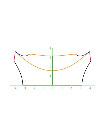
For the sake of visualization, in Figure 8, we show a cross-section of for .
In general, the situation is similar for . For , the degenerate boundary shrinks only to ; and there is no degenerate boundary for . Now, contains two such bands, and is two such band glued together (all meant for a fixed ). In this setting contains two segments, and is a circle.
Another sort of blow-up which affects the variables is given by passing to the coordinates such that , and
| (90) |
In merit, as a blow-up, this affects only the case of the zero-boundary (where it is slightly advantageous). As such, its use is marginal for us. However, (90) is retained as a practical change of coordinates, which is particularly useful if is kept fixed.
Lemma 8.5.
In the context of Lemma 8.3 and Lemma 8.4, the extended actions on some boundary pieces (restricted for a fixed , with ) are given as follows:
(a) If (so ), i. e. we consider the Schur-hyperbolic boundary , then
Here is arbitrary.
The normalized expressions extend as
and (if ,)
These curves (in ) are two-sided -hypercycles (-distance lines).
(b) If (so ), i. e. we consider the purely elliptic boundary , then
Here the domain restriction can be expressed as
The normalized expressions extend as
and (if ,)
These curves (in ) in the CKB model are radially contracted images of (possibly two open pieces of) the unit circle. (They give quasi Cassini ovals.)
(c) If , i. e. we consider (in particular ), then
The domain restrictions are expressed as
The extended actions are given by
and
In particular, the image of is
and
(For , this is just the origin, which comes from . For , the endpoints come from , the origin comes from , the intermediate points come from .)
(d) If , i. e. we consider , or rather , then
and
The absolute values of the seconds coordinates are strictly monotone increasing in ,
and
(The lower limits come from , the upper limits come from , the intermediate values come from .
Proof.
Direct computation. ∎
For the sake of visualization, in Figure 8, we show pictures about the range of restricted to and to a fixed , with parameter lines induced by and , for the cases , , , ; and the image of the relevant boundary pieces in the cases , . Furthermore, in Figure 8, we also include a picture about the corresponding range of in the case .
We see the following: Through , the various components of map as follows:
The Schur-hyperbolic boundary (i. e. , ) maps injectively to the outer rim.
The Schur-elliptic boundary (i. e. , ) maps injectively to the inner rim except to the origin.
The closure of the pseudoboundary (i. e. ) gives two pinches on the sides. (This is improved by , which is injective on .)
The degenerate boundary maps to the inner slit. More precisely:
For , there is no degenerate boundary.
For , the degenerate boundary is , it maps to the origin.
For , the degenerate boundary is (restricted to norm ). Then maps to the upper and lower tips of central slit, maps to the origin, maps to join them.
The red lines: varies, (or ) is fixed. The blue lines: (or ) varies, is fixed. It is quite suggestive that maps injectively into two simply connected domains, but this requires some justification, which is as follows.
In fact, the proof of the next lemma will introduce some important computational techniques:
Lemma 8.6.
Suppose that .
(a) Let be the subset of which contains the elements of norm . Then the operations and (cf. (85)) are injective on .
(b) Let be the subset of which is the restriction to . Then the operation (cf. (86)) is injective on .
In fact, its image is the union of two simply connected domains bounded by the image of the boundary pieces , laying in the upper and lower half-planes, respectively.
Proof.
Due to the circular fibration property, it is sufficient to prove (b). By the monotonicity properties of the boundary pieces (cf. Lemma 8.5) one can characterize the simply connected domains. Then one can check that (or ) start to map into the two simply connected domains near the boundary pieces, which is tedious but doable. (It requires special arguments only in the case of ; see comments later.) Then, for topological reasons, it is sufficient to demonstrate that the Jacobian of (or ) on never vanishes.
Then, it is sufficient to consider the model. We have to compute the Jacobian of
with
with respect to ( is fixed) subject to , . We find
| (91) | ||||
where the arguments of should be . Each summand is non-positive; in fact, strictly negative, with the possible exception of the last one. Thus the Jacobian is negative.
Moreover, this method with the Jacobian applies to around (i. e. , ) and (i. e. , ) as (91rhs/1) is always negative. Moreover, it also applies to and where (91rhs/1)–(91rhs/3) extend to zero smoothly but (91rhs/4) gives an nonzero contribution.
In fact, if we pass to , then it becomes regular even near the asymptotical points: It yields
| (92) |
This extends smoothly to the case , i. e. to . It is easy to see that, on this set, the Jacobian is strictly negative again. (Note that in this case , thus and are positive.)
This still leaves the uneasy case of regarding boundary behaviour. However, even those cases can be handled, as failure of indicated behaviour at those point (1-1 points for each simply connected domain for a fixed ) would cause irregular behaviour at other points. ∎
The following discussion will be important for us. For , we let
One can immediately see that
that is
On the other hand,
Lemma 8.7.
Proof.
By direct computation one can check that
(The arguments of should be .)
Then the statement follows from the observation that every term in the sum is strictly negative on the specified domain. ∎
Here an important observation is that depends solely on , and, by homogeneity, only on . Similar definitions, statements, and observations can be made regarding , and .
Remark 8.8.
Let us address the question that whether and can be extended to formally beyond the already discussed cases.
(o) If such that
| (93) |
then extends by the formula
where
and
and
and
and
This dispenses with the condition (81).
(a) If , , then can be replaced by an arbitrary . Formally, this leads to
where is undecided. Here
and
and
and
and
(The undecidedness of does not appear .)
(b) If , , then becomes undecided. Here
and
and
and
and
(The undecidedness of does appear .)
These calculations were formal. The real geometrical picture is computed in what follows. “Undecidedness” will appear as conical degeneracy. ∎
Lemma 8.9.
Suppose with (thus ) and . Then
In particular, if
then
(For , should be understood as .)
Proof.
Direct computation. ∎
Lemma 8.10.
Suppose , , and . Then
In particular, if
then
Similarly,
In particular, if
then
Proof.
Direct computation. ∎
Lemma 8.11.
Suppose that , and, in particular, or . Let . Then
Proof.
Direct computation. ∎
9. BCH minimality
Definition 9.1.
We say that is a BCH minimal pair (for ), if for any such that it holds that or .
In this section we seek restrictions for BCH minimal pairs.
Any element can easily be perturbed into the product of two -able elements (for example, one close to and one close to ). By a simple compactness argument we find: If , then allows a minimal pair such that and . In minimal pairs, however, we can immediately restrict our attention to some special matrices:
By Lemma 8.1, all minimal pairs are from . By the same lemma, we also see that the elements of and are all minimal pairs.
Definition 9.2.
Assume that . We say that is an infinitesimally minimal BCH pair, if we cannot find such that
| (94) |
Lemma 9.3.
Assume that , and is not infinitesimally minimal. Then one can find such that
yet
In particular, infinitesimal minimality is a necessary condition for minimality.
Proof.
If (94) holds, the let and with a sufficiently small . ∎
Lemma 9.4.
Suppose that such that and are not positive multiples of each other. Then the pair is not infinitesimally minimal; in particular, is not minimal.
Proof.
The the nonzero linear functionals and are not positive multiples of each other, thus one can find such that (94) holds. ∎
Lemma 9.5.
If is BCH minimal, then .
Proof.
For , and are inner points CKB, for , and are asymptotic points CKB. From this, and the previous lemma, if is infinitesimally minimal, then or . Regarding the second case, by infinitesimal minimality, is required. Then we can take , and, by Lemma 8.7, and will give a counterexample to BCH minimalty with a sufficiently small . ∎
Lemma 9.6.
Suppose that is an infinitesimally minimal BCH pair. We claim:
(a) If , then .
(b) If , then or or .
(c) If , then or or .
Proof.
(a) By Lemma 8.11, for the relation holds . (‘ ’ means ‘approximately’.) Then the statement is a consequence of Lemma 9.3, and furthermore, Lemma 8.9.
(b) and (c) follow from the observation that the maps and , if they are linear functionals, should be proportional to each other (cf. Lemma 9.3). ∎
By taking adjoints, the relation described in the previous lemma is symmetric in and . This leads to
Theorem 9.7.
For minimal BCH pairs, where all factors are of positive norm, one has the following incidence possibilities:
Here means ‘perhaps possible’, and means ‘not possible’.
Proof.
This is a consequence of the previous statements. ∎
Next, we obtain more quantitative restrictions.
Lemma 9.8.
(a) For consider the pairs
or
where . Then the pairs will produce, up to conjugation by rotation matrices, every (infinitesimally) BCH minimal pair from . In these cases
(b) Similar statement holds for with respect to .
Proof.
(a) By infinitesimal minimality, the matrices should be aligned. BCH minimality follows from Magnus minimality. (b) This is a trivial extension of (a). ∎
Lemma 9.9.
Consider the function given by
and the linear functional given by
Then we can choose such that and unless
| (95) |
holds, in which case finding such a is impossible.
Proof.
If , or , or , or , then
or
or
or
respectively, are a good choices.
(In merit, this is just a simple geometrical statement about a half-cone.) ∎
Lemma 9.10.
Suppose that , , and , where . Suppose that is infinitesimally BCH minimal. Then
and
| (96) |
(For the , the LHS is understood as , but then the condition is vacuous anyway. Also note that the condition is imposed by .)
Lemma 9.11.
Suppose that , , and , where . If is infinitesimally BCH minimal, then
and
| (97) |
Lemma 9.12.
Suppose that and . Assume that and . Let denote the angle between the vectors and . We claim that if is an infinitesimally BCH minimal pair, then , and
| (98) |
Proof.
(By conjugation we can assume that
Then direct computation yields the statement.) ∎
Assume that is a subset of closed under conjugation by rotation matrices. Then the set is also closed conjugation by rotation matrices. Thus it can be represented by its image through accurately. We say that set has a factor dimension , if the map applied to it can be factorized smoothly through a smooth manifold of dimension .
Theorem 9.13.
Factor dimensions of the BCH minimal subsets of the sets restricted to , , are
Remark.
The numbers given are sort of upper estimates, but one can see that one cannot reduce them generically. ∎
Proof.
The previous statements and simple arguments show this. E. g. Lemma 9.10 takes care to , etc. ∎
Furthermore, note that the image of the restriction of contains the images of the restrictions of and , which contain the image of the restriction of (and also in reverse order).
Note that is surely well-defined if and (as the BCH presentation is not Magnus-minimal).
Lemma 9.14.
Consider the map with , , . (Thus and .) We claim:
(a)
(b) is log-able if and only if
(c) In the log-able case: Let denote the projection to the second and third coordinates. Then, for the Jacobian,
where the arguments of and should be .
In particular, this is non-vanishing if .
Proof.
(a) This is direct computation. (b) This is a consequence of Lemma 2.14(a).
(c) The formula for can be applied, then direct computation yields the result. Regarding non-vanishing, we can see that beyond , all multiplicative terms are positive. ∎
Note that is surely well-defined if and (as the BCH presentation is not Magnus-minimal).
Lemma 9.15.
Consider the map with , , . (Thus and .) We claim:
(a)
where
such that the arguments of and should be .
(b) is log-able if and only if
where are as before.
(c) In the log-able case: Let denote the projection to the second and third coordinates. Then, for the Jacobian,
where are as before, and
and the arguments of and should be .
In particular, this is non-vanishing if .
Proof.
(a) is direct computation. (b) is a consequence of Lemma 2.14(a). (c) The formula for can be applied, then direct computation yields the result. Regarding non-vanishing, we can see that beyond , all multiplicative terms are positive. ∎
Let denote either or . It would be desirable to show that
(SEHC1) “If and then
has no local extremum.”
A statement which would provide this can be formulated as follows. For , let . One can recognize it as a sort of the gradient of norm. Then a stronger statement is
(SEHC2) “If and then
and
| (99) |
(the standard vectorial product is meant) are not nonnegatively proportional.”
An even stronger possible statement is as follows. For , let be defined by
(SEHC3) “If and , then the Jacobian
is nonvanishing.”
This latter statement can be established in particular cases (for and ) but I do not know a general argument.
Remark 9.16.
For ,
seems to be the case (for and fixed). For ,
seems to hold. These estimates can be established in several special cases. ∎
10. The balanced critical BCH case
Let . Consider
This is not a closed set. The reason is that is not defined at , thus the usual compactness argument does not apply. This failure in well-definedness affects only two cases, and . Yet, the closure is larger than by several quasi -s of , as Theorem 7.1 shows. (In this setting, is the same as except the latter one is well-defined everywhere but still non-continuous at the critical points. Thus, a quite legitimate version of the set above is its union with .)
Theorem 10.1.
(a) The elements of
are exactly the elements which are are of shape
with
and
(b) The elements of
are all of shape with and such that is a BCH minimal pair.
(c) The interior of is connected, containing .
Proof.
(a) The set should be closed to conjugation by orthogonal matrixes, and by continuity of , theirs exponentials are . Then only the norms are of question but Theorem 7.1 takes care of that. (b) , (c) These follow from the openness of as long as the domain is restricted to the spectrum in . ∎
The set is closed for conjugation by orthogonal rotations, thus it can be visualized through . Then , expectedly a -dimensional object, describes . In the previous section we have devised several restrictions for (infinitesimally) BCH minimal pairs. In fact, we find that must be contained in the union of continuous images of finitely many, at most dimensional, manifolds, which can described explicitly. Despite this, computation with these objects is tedious.
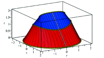
Therefore we restrict our attention to the case (i. e. ), which is the most important for us. Before giving any argument, by the following Figure 10, let us show what we will obtain:
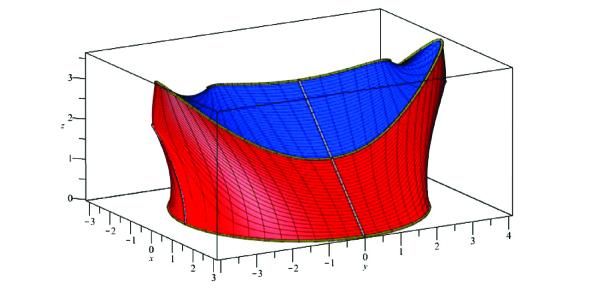
\phantomcaption
is a “wedge cap”. What see is the following (note that here):
In the middle top, we see the Schur bihyperbolic ridge, the image of the (infinitesimally) minimal pairs from .
Joining it, we see Schur parabolical segments (in the -plane), the image of the (infinitesimally) minimal pairs from .
The middle ridge is the Schur elliptic-hyperbolic ridge, the image of the (infinitesimally) minimal pairs from or (transposition invariance shows equality).
In the front and back see we the closure singularity segments (in the -plane), the images coming from limiting to
In the very bottom, we see the Schur bielliptic rim, the image of the (infinitesimally) minimal pairs from and , but of which are exceptional (that is the former case is eliminated).
The upper, blue area is the Schur smooth-hyperbolic area, the image of the (infinitesimally) minimal pairs from or . (Again, note transposition invariance.)
The lower, red area is the Schur smooth-elliptic area, the image of the (infinitesimally) minimal pairs from or .
Remark 10.2.
The situation with with is similar, cf. Figure 10.2,
except the “closure” singularity does not develop. ∎
Let us now make the “statement” of Figure 10 more precise. Let us fix the choice .
We define the Schur bihyperbolic parametrization as the map
We define the Schur parabolic parametrization as the map
We define the Schur elliptic*-hyperbolic parametrization as the map
We define the closure parametrization as the map
We define the Schur bielliptic parametrization as the map
We define the Schur smooth-hyperbolic parametrization as the map
(Here we have used the abbreviations of Lemma 8.2.)
Similarly, we define the Schur smooth-elliptic parametrization as the map
We will call these maps as the canonical parametrizations in the case.
Remark 10.3.
For , the canonical parametrizations can defined similarly in the case, except the situation is simpler: These is no closure parametrization but the Schur bielliptic parametrization can be defined fully for . ∎
Theorem 10.4.
(a) Every element of occurs the image of BCH minimal pair with respect norms with the exception of the closure singularities. Conversely, every image of a such a BCH minimal pair or a point of the closure singularity is in .
(b) The canonical parametrizations taken together map to bijectively, and the images fit together topologically as suggested by Figure 10.
Proof.
First we prove that non BCH minimal points map to the interior. Indeed as least one component can be replaced by an element of norm less then . As the exponential map and the logarithm will be open in these circumstances, perturbing that the entry yields an open neighborhood in the image. This proves the first part of (a). The second part, and, in fact, the rest of the statement, follows by topological reasons if we prove that the images of the canonical maps fit together topologically as a half-sphere. For the 1-dimensional canonical parametrizations injectivity and topological incidences are easy to check. Next one can prove that the 2-dimensional parametrizations limit on their boundary in an expected manner. In that blow-ups in ACKB or AHP are instrumental, except at the pairs , continuity (in fact, well-definedness) breaks down. Yet, we know that the limits exponentiate to , and we know the range of the norm by Theorem 7.1. By this, the closure singularies can be recovered. Also, the sign relations in (the trace) coordinate are easy due to the BCH formula. To the 1-dimensional canonical parametrization we can add the cases of the smooth-hyperbolic and smooth-elliptic canonical parametrizations. By the sign relations in , then it is sufficient to prove that -projections of the parts of smooth-hyperbolic and smooth-elliptic canonical parametrizations have non-vanishing Jacobians. Thus the fill out the corresponding regions in Figure 10(c) as they should. (That also shows that they fit to the closure singularities properly.) ∎
Theorem 10.5.
(Here the exceptional cases and do not participate in the supremum. But, writing , they could.)
Indication of proof.
Thus, one has to prove
According to Theorem 10.1, we can replace by , in fact, by . By various estimates, we can localize the maxima near to tip of the horns of Figure 10(a). By further estimates, one show that the direction of gradients for the Schur smooth-elliptic parts and Schur smooth-hyperbolic parts near the tip are inconsistent to the maxima. Thus it remains to optimize on the Schur elliptic*-hyperbolic part. There, ultimately, we obtain the tips as expected for the maxima. ∎
Remark 10.6.
In the previous proof, the critical part is the reduction to the 1-dimensional boundary pieces. In a less ad hoc way it is also achieved by showing, say, (SECH3) for , which is quite doable as a special case. For 1-dimensional optimizations there are just several methods. ∎
It seems reasonable to expect that
(SM0) “If and , then the maximum of for is taken for a traceless pair of matrices.”
Indeed, large norm seems to come from non-commutativity, and thus including tracial parts seems to be quite pointless. Again, this is quite provable in several special cases, but I do not know a general proof. It may be possible, however, that a quite simple argument will suffice.
Remark 10.7.
The localizations of the maxima, however, are not trivial even in the case . Indeed, in this setting, there is a critical value
such that for , the maxima are taken on the Schur bihyperbolic ridge (cf. Figure 10.2); and for , the maxima are taken on the Schur elliptic*-hyperbolic ridge; and for , on both. ∎
Thus one can expect that
(SM+) “If and but is sufficiently large, then the maximum of for is taken for a traceless Schur elliptic-hyperbolic pair, the norm of the conform-involution is less or equal than the norm of conform-skew-involution.”
However, this needs further exploration.
Remark 10.8.
If this is true, then Example 6.4 seems to be sharp case. ∎
11. Principal disks and logarithm
Lemma 11.1.
Suppose that is a -able real matrix with principal disk
In that case,
| (100) |
and
| (101) |
where
and
In particular, if , then , and , .
Theorem 11.2.
Suppose that are -able real matrices such that
Then
| (102) |
and
| (103) |
Remark.
The monotonicity of is strict, except if and are centered on the real line and .
The monotonicity of is strict, except if and are centered on the real line and . ∎
Proof.
Let denote the functional expression on the right side of (100). Then it is a straightforward but long computation to check the identity
| (104) |
This is valid, except if and , the exceptional configurations. In particular, if , then
The principal disks with form a connected set, consequently
| (105) |
or
should hold globally for . The question is: which one? It is sufficient to check the sign at a single place. Now, it is not hard to check that
(except if ), which shows that (105) holds. The meaning of (105) is that expanding principal disks smoothly with non-real centers leads to growth in the norm of the logarithm.
Let us return to principal disks in the statement. If , then we can expand the smaller one to the bigger one with non-real centers. (Indeed, magnify from its lowest point, until the perimeters touch, and then magnify from the touching point.) This proves the (102) for . The general statement follows from the continuity of the norm of the logarithm. Notice that the norm grows if we can expand through .
Lemma 11.3.
Suppose that are real matrices. Then
holds if and only if
and
Proof.
The norms and co-norms can be read off from the principal disk immediately. Hence the statement is simple geometry. ∎
Theorem 11.4.
Suppose that are -able real matrices. If
then
The monotonicity is strict. Similar statement applies to .
Proof.
In this case, the matrices will also be -able. Moreover, holds. Now, . By the previous theorem, and holds for every . According to the previous lemma, this implies the main statement. The monotonicity is transparent in this case, as both and are compatible with conjugation by orthogonal matrices, hence the orbit correspondence is one-to-one. respects chirality, hence the statement can also be transferred to chiral disks. ∎
12. Examples: The canonical Magnus developments in
Example 12.1.
(Magnus parabolic development.) On the interval , consider again the measure , such that
Then, for ,
Here
Thus
Consequently,
As
| (106) |
As ,
| (107) |
This is not only better than (9), but it has the advantage that it can be interpreted in terms of the solution of a differential equation blowing up. ∎
Example 12.2.
(Magnus elliptic development.) Let be a parameter. On the interval , consider the measure such that
Then, for
It is easy to see that
Here . We find that
Thus, if , then
It is notable that
which is contracted from the boundary point by factor . ∎
Example 12.3.
(Magnus hyperbolic development.) More generally, let be a real parameter. On the interval consider the measure , such that
Then, for
is the same as , and . If , then
| (108) |
Consequently,
| (109) |
Remark 12.4.
For and ,
holds. (Understood as for . It is also for .) Thus, under these assumptions, the absolute value in (109) is unnecessary. ∎
13. Magnus minimality in the case
Theorem 13.1.
Let . Consider the family of disks parameterized by , such that the centers and radii are
for ; and
(a) The circle is tangent to at
These points are inverses of each other relative to the unit circle. If the points are equal (), then the disk is the osculating disk at .
The disks themselves are orthogonal to the unit circle. The disks are distinct from each other. Extending , we have , .
(b)
(c) The disks are the maximal disks in . The maximal disk touches only at , .
Proof.
(a) The disks are distinct because, the centers are distinct: For ,
(Cf. ) The rest can easily be checked using the observation
(b) This is direct computation.
(c) In general, maximal disks touch the boundary curve , and any such touching point determines the maximal disk. (But a maximal disk might belong to different points.) Due to the double tangent / osculating property the given disks are surely the maximal disks, once we prove that they are indeed contained in . However, together with Theorem 1.2 implies that . The distinctness of the circles implies that they touch the boundary only at the indicated points. ∎
Alternative proof for ..
Here we give a purely differential geometric argument.
One can see that the given disks are characterized by the following properties:
() If , then the disk is tangent to at these points.
() If , i. e. , then the disk is the osculating disk at .
Now, we prove that . First, we show that . Indeed,
hence, by Theorem 1.2, the of any element of is contained in
Let be the maximal real number such that for any , and . (Due to continuity, there is a maximum.) Indirectly, assume that . Then one of following should happen:
(i) Besides and there is another pair (due to inversion symmetry) of distinct points and , where touches the boundary of .
(ii) touches the boundary at or .
(iii) is osculating at or at .
(Symmetry implies that are equally bad.) Case (i) is impossible, because the given circles are distinct and the characterising properties hold. Case (ii) is impossible, because, due to and the extremality of , the situation would imply that strictly contains the osculating disk at or , which is a contradiction to . Case (iii) is impossible, because for the oriented plane curvature of ,
holds if . (In general, for .) This implies , proving the statement. ∎
In what follows, we will not make much issue out of expressions like when ; we just assume that they are equal to , in the spirit of continuity.
Theorem 13.2.
Suppose that . Suppose that is a disk in , which touches at . Then for an appropriate nonnegative decomposition ,
The bigger the is, the bigger the corresponding disk is. corresponds to the maximal disk, corresponds to the point disk.
Proof.
Let denote the argument of . Then its first component is Magnus exponentiable by norm , and its second component is Magnus exponentiable by norm . Thus the principal disk must lie in . One can compute the center and the radius of the chiral disk (cf. the Remark), and find that is on the boundary of the disk. So, must be the maximal contracted from . One, in particular, finds that the radius of is
This shows that bigger leads to bigger disk. ∎
Remark.
It is easy to see that, for ,
This immediately implies the existence of a certain normal form. For the sake of compact notation, let
which is the set of the conjugates of by orthogonal matrices.
Theorem 13.3.
Suppose that such that . Assume that is the smallest real number such that , and touches at . Then there is an nonnegative decomposition , and a matrix , such that
| (111) | ||||
| (112) | ||||
| (113) | ||||
| (114) |
The case corresponds to .
The case corresponds to point disk case, the expression does not depend on .
The case corresponds to the maximal disk case, it has degeneracy .
In the general case , the presentation is unique in terms of .
Proof.
This is an immediate consequence of the previous statement and the observation ∎
In what follows, we use the notation
to denote the arithmetic expression on the RHS of (111). In itself, it just a matrix value, but the statement above offers three particularly convenient ways (normal forms) to present is as a left-exponential: (112) is sufficiently nice and compact with norm density on an interval of unit length. (113) and (114) are concatenations of intervals of length and with norm density . One part is essentially a complex exponential, relatively uninteresting; the other part is the Magnus parabolic or hyperbolic development of Examples 12.1 and 12.3, but up to conjugation by a special orthogonal matrix, which is the same to say as ‘up to phase’.
Theorem 13.4.
Suppose that such that . Then
Or, in other words,
Suppose that such that , , . If , then can be of the three kinds: Magnus elliptic, when touches at or , but it is not an osculating disk; Magnus parabolic, when touches at or , and it is an osculating disk; or Magnus hyperbolic when touches at two distinct points. If then touches at a single point, asymmetrically; we can call these Magnus loxodromic. We see that Examples 12.1, 12.2, and 12.3, cover all the Magnus parabolic, hyperbolic and elliptic cases up to conjugation by an orthogonal matrix. In general, if is not Magnus hyperbolic, then it determines a unique Magnus direction (in the notation Theorem 13.3). It is the direction of the farthest point of from the origin. If is Magnus hyperbolic, then this direction is determined only up to sign in the real part.
Lemma 13.5.
Suppose such that , , , . Then and .
We claim that is Magnus hyperbolic or parabolic if and only if
If is Magnus elliptic or parabolic, then
Proof.
intersects the unit circle at
. In particular, ; multiplying them, we get . Then . If one them is equal to , then it is a Magnus parabolic case; if those are smaller than , then it is a Magnus hyperbolic case; if one of them is bigger than , this it must be a Magnus elliptic case. (Cf. the size of the chiral disk in Theorem 13.2.) ∎
Recall that we say that the measure is a minimal Magnus presentation for , if and .
Lemma 13.6.
Any element has at least one minimal Magnus presentation.
Proof.
is connected, which implies that any element has at least one Magnus presentation . If is small enough, then we can divide the supporting interval of into many subintervals, such that the variation of on any of them is less than . Replace by a normal form on every such subinterval. By this we have managed to get a presentation of variation at most by a data from . Conversely, such a data always gives a presentation, whose depends continuously on the data. Then the statement follows from a standard compactness argument. ∎
Lemma 13.7.
Suppose that , such that is Magnus hyperbolic, but for any . Suppose that .
Then, as the sequence converges,
or more precisely,
Proof.
We can assume that . From the formula of one can see that is an entire function of . One actually finds that the center is
(One can check that in the expansion , every term is divisible by ; in the expansion , every term is divisible by .) Eventually, one finds that
and
The hyperbolic developments are uniform motions in the sense that the increments differ from each other by conjugation by orthogonal matrices as changes. In fact, they are locally characterized by the speed , and a phase, i. e. conjugation by rotations.
Lemma 13.8.
Assume that ; ; ; . On the interval , consider the measure given by
where
Then
unless and .
Proof.
It is sufficient to prove this for a small subinterval around . So let us take the choice , . Then
Let
(i) If , then
This shows that gets Magnus elliptic. However,
shows Magnus non-minimality.
(ii) If , , then
This also shows Magnus ellipticity, and
shows Magnus non-minimality.
(iii) If , , then . Hence, full cancellation occurs, this is not Magnus minimal.
(iv) If , , then , and
This shows that gets Magnus hyperbolic. Then, assuming Magnus minimality and using the previous lemma, we get a contradiction by
This proves the statement. ∎
Lemma 13.9.
Assume that ; ; . On the interval , let us consider the measure given by
where
Then
Proof.
Again, it is sufficient to show it for a small subinterval around .
(i) Suppose . As , restrict to the interval
Then
Let
If we assume Magnus minimality, then
Thus, is Magnus parabolic. By direct computation, we find
in contradiction to
which is another way to express from the density. (The coefficients of differ for .)
(ii) Consider now the case .
shows Magnus ellipticity, and
shows non-minimality. ∎
Now we deal with the unicity of the normal forms as left exponentials. In the context of Theorem 13.3 we call the elliptic component of , and we call the hyperbolic length of .
Theorem 13.10.
Suppose that such that , and is a minimal Magnus presentation for supported on .
Then, restricted to any subinterval , the value is a multiple of by a nonnegative real number. Furthermore the interval functions
are additive. In particular, if is Magnus hyperbolic or parabolic, then is always .
Proof.
Let us divide the supporting interval of into smaller intervals . On these intervals let us replace by a left-complex normal form. Thus we obtain
where are are some intervals, and are hyperbolic developments (up to conjugation). (They can be parabolic but for the sake simplicity let us call them hyperbolic.) Further, rearrange this as
where the hyperbolic developments suffer some special orthogonal conjugation but they remain hyperbolic developments. Now, the elliptic parts
must be nonnegatively proportional to each other, otherwise cancelation would occur when the elliptic parts are contracted, in contradiction to the minimality of the presentation. By this, we have proved that in a minimal presentation elliptic parts of disjoint intervals are nonnegatively proportional to each other.
Suppose that in a division occurs. Contract the elliptic parts in but immediately divide them into two equal parts:
Now replace everything but the last term by a normal form
Taking the determinant of the various left-exponential term we find
Thus , hence, by minimality , moreover . However, the constitutes a normal form (prolonged in the elliptic part), which in this form is unique, thus, eventually
| (115) |
must hold.
Suppose now that or occurs with . Consider . By Magnus minimality and Lemma 13.8, the hyperbolic development must fit into single hyperbolic development (without phase or speed change). Furthermore, by Lemma 13.9, must be parabolic fitting properly to the elliptic parts. Thus , in fact, yields a normal form . Then (115) holds.
The third possibility in is that all the intervals are of zero length. Then the hyperbolic developments fit into a single development , but (115) also holds.
Thus (115) is proven. It implies nonnegative proportionality relative to the total . Now, subintervals of minimal presentations also yield minimal presentations, therefore additivity holds in full generality. Regarding the interval functions, the additivity of is trivial, the additivity of is just demonstrated, and is just the minus the absolute value (norm) of . ∎
Remark 13.11.
Suppose that is a measure. Assume that is a subinterval such that . Let us replace by a Magnus minimal presentation of , in order to obtain an other measure . Then we call a semilocal contraction of .
We call semilocally Magnus minimal, if finitely many application of semilocal contractions does not decrease . (In this case, the semilocal contractions will not really be contractions, as they are reversible.) We call locally Magnus minimal, if any application of a semilocal contraction does not decrease . It is easy to see that
The arrows do not hold in the other directions. For example, is semilocally minimal but not Magnus minimal. Also, is locally Magnus minimal but not semilocally Magnus minimal: Using semilocal contractions we can move and beside each other, and then there is a proper cancellation.
The proper local generalization of Magnus minimality is semilocal Magnus minimality. If is locally Magnus minimal, the we can define and by taking a finite division of of to intervals of variation less than , and simply adding and . What semilocality is needed for is to show that is nonnegatively proportional to , and to a proper definition of the Magnus direction of .
Having that, semilocally Magnus minimal presentations up to semilocal contractions behave like Magnus minimal presentations. They can also be classified as Magnus elliptic, parabolic, hyperbolic, or loxodromic. (But they are not elements of anymore but presentations.) In fact, semilocally Magnus minimal presentations up to semilocal contractions have a very geometrical interpretation, cf. Remark 13.15. (Interpreted as elements of .) ∎
As Theorem 13.3 suggests, hyperbolic and parabolic developments are rather rigid, while in other cases there is some wiggling of elliptic parts.
Theorem 13.12.
Suppose that , , and is a minimal presentation to supported on the interval .
(a) Suppose that is Magnus hyperbolic or parabolic. Then there are unique elements and such that
Thus, minimal presentations for Magnus hyperbolic and parabolic matrices are unique, up to reparametrization of the measure.
(b) Suppose that is point disk. Then there is a unique element such that
Thus, minimal presentations for quasicomplex matrices are unique, up to reparametrization of the measure.
(c) Suppose that is not of the cases above. Then there are unique elements , , , and surjective monotone increasing function such that
and
Thus, minimal presentations in the general case are unique, up to displacement of elliptic parts.
Proof.
Divide to and , and replace the minimal presentation by norma forms. They must fit in accordance to minimality. ∎
Remark.
The statement can easily be generalized to semilocally Magnus minimal presentations. ∎
Theorem 13.12 says that certain minimal Magnus presentations are essentially unique. Theorems 13.13 and 13.14 will give some explanation to the fact that it is not easy to give examples for the Magnus expansion blowing up in the critical case .
Theorem 13.13.
Suppose that , , and is a minimal presentation to supported on the interval . If is of shape
with some matrix (i. e., it is essentially an exponential), then is a normal matrix with norm .
Proof.
Due to homogeneity, and must be proportional to . But it is easy to see that (up to parametrization) only the homogeneous normal densities (112) have this property, and they are locally constant only if the Magnus non-elliptic component vanishes with , or when they are of special hyperbolic type with . ∎
(This redevelops Theorem 5.1 in the real case.)
Theorem 13.14.
Suppose that is a measure,
but does not exist. Then there are uniquely determined elements and , a nonnegative decomposition , with , and surjective monotone increasing functions such that
and
Thus, critical cases with blowing up are the Magnus elliptic and parabolic (but not quasicomplex) developments up to reparametrization and rearrangement of elliptic parts.
Proof.
The presentation must be Magnus minimal, otherwise the would be OK. Divide to and , and replace the minimal presentation by normal parts. They must fit in accordance to minimality. It is easy to see that in the Magnus hyperbolic / loxodromic cases has no chance to reach . The disks are the largest in the Magnus hyperbolic cases, and the chiral disks of Magnus strictly hyperbolic developments do not reach the negative axis. So the Magnus elliptic and parabolic cases remain but the quasicomplex one is ruled out. ∎
Thus, even critical cases with are scarce.
Remark 13.15.
We started this section by investigating matrices with . It is a natural question to ask whether the treatment extends to matrices with, say, . The answer is affirmative. However, if we consider this question, then it is advisable to take an even bolder step:
We can extend the statements for , the universal cover of . This of course, implies that we have to use the covering exponential and should also be replaced by . Now, the chiral disks of elements of live in , the universal cover of .
Mutatis mutandis, Theorems 13.1, 13.2, 13.3 extend in a straightforward manner. Remarkably, Theorems 1.1 and 1.2 have versions in this case (the group acting on the universal cover of ), however we do not really need them that much, because chiral disks can be traced directly to prove a variant of Theorem 13.4. Elements of also have minimal Magnus presentations. In our previous terminology, they are semilocally Magnus minimal presentations. In fact, semilocally Magnus minimal presentations up to semilocal contractions will correspond to elements of . Their classification to Magnus hyperbolic, elliptic, parabolic, loxodromic, quasicomplex elements extends to . This picture of helps to understand . Indeed, we see that every element of have countably many semilocally Magnus minimal presentations up to semilocal contractions, and among those one or two (conjugates) are minimal. The Magnus exponent of an element of is the minimal Magnus exponent of its lifts to . ∎
Example 13.16.
Let be the solution of on the interval . Consider
The determinant of the matrix is , we want to compute its real Magnus exponent. The optimistic suggestion is . Indeed, in the complex case, or in the doubled real case, this is realizable from
However, in the real case, there is “not enough space” to do this. A pessimistic suggestion is . Indeed, we can change sign by an elliptic exponential, and then continue by a hyperbolic exponential. This, we know, cannot be optimal. In reality, the answer is . In fact, is Magnus parabolic, one can check that . This is easy to see from the chiral disk.
In this case there are two Magnus minimal representations, because of the conjugational symmetry. ∎
14. Optimal asymptotical norm estimate for
If is an ordered valued measure with cumulative norm such that , then, according to the previous sections, the maximal possible norm of its Magnus expansion is realized via maximal disks, through canonical Magnus parabolic or hyperbolic developments. Thus this maximal norm is of shape where . Thus we have optimize in , although at this point it is not clear that is unique depending .
Using the implicit function theorem, however, it is easy to see that, for , the optimal ridge is defined with , where
Then
| (116) |
We see that this is somewhere in the middle, below the upper estimate (7) and above the parabolic case (106); but all deviations are of .
Using an appropriate reparametrization and the implicit function theorem, one can see that, for , the optimal ridge is defined with , where
Then
| (117) |
This is below the upper estimate (8) by , and above the parabolic case (107) by , and above the lower estimate (110) by .
It is natural to ask whether the general upper estimate can be improved to, say
as .
Remark 14.1.
One can show that yields a well-defined analytic function for . This is, however, complicated, as it requires global estimates. ∎
15. A counterexample for complex matrices
According to Theorem 13.4, , , and implies that with some appropriate such that . Here we demonstrate that the corresponding statement is not valid for complex matrices.
Let . In the CKB model, we will consider the Magnus range
Then it is easy to see that its hyperbolic boundary
is parametrized by the curve
The tangent line at is given by the equation
(In this section, are understood as .) Note that , , .
It is not hard to see that the equation of the ellipse tangent to at the three parameter points is given by
(the coefficient of is nonnegative).
Example (Proposition) 15.1.
For the choice
the elliptical disk
is realized as the conformal range of a complex matrix in CKB (i. e. as ). Regarding this (4 different cases up to unitary conjugation),
but
| (118) |
Proof.
One can check that, for the given choice, the ellipse lies in the interior of the unit circle, thus it be realized as the boundary of the conformal range of a (purely complex) complex matrix . (Cf. Davis [5],[6], Lins, Spitkovsky, Zhong [14], or, in greater detail, [13].) It is harder to see but this ellipse lies in , intersecting (tangent to) at . (This requires checking the second derivatives near the critical points, and for the rest numerical considerations are sufficient.)
Assume that now with . Then allows an initial restriction such that . Let . Then, however, implies that that . In this case should be the ellipse with boundary . One can, on the other hand, check that this ellipse is not in the unit circle, which is a contradiction.
In fact, if we allow with (with small ), then it still means that the boundary of should pass through certain points near but contained in (making the tangents also close at the given points). This still makes the boundary of close to , yielding a contradiction. (Thus (118) could be quantified further.) ∎
References
- [1]
- [2] Berger, Marcel: Geometry I, II. Universitext. Springer-Verlag, Berlin, 1987.
- [3] Bonfiglioli, Andrea; Fulci, Roberta: Topics in noncommutative algebra. The theorem of Campbell, Baker, Hausdorff and Dynkin. Lecture Notes in Mathematics, 2034. Springer, Heidelberg, 2012.
- [4] Casas, Fernando: Sufficient conditions for the convergence of the Magnus expansion. J. Phys. A 40 (2007), 15001–15017.
- [5] Davis, Chandler: The shell of a Hilbert-space operator. Acta Sci. Math. (Szeged) 29 (1968), 69–86.
- [6] Davis, Chandler: The shell of a Hilbert-space operator. II. Acta Sci. Math. (Szeged) 31 (1970) 301–318.
- [7] Gans, David: A new model of the hyperbolic plane. American Math. Monthly 73 (1966), 291–295.
- [8] Goldberg, Karl: The formal power series for . Duke Math. J. 23 (1956), 13–21.
- [9] Kreĭn, M. G.: The angular localization of the spectrum of a multiplicative integral in Hilbert space (In Russian). Funkcional. Anal. i Priložen. 3 (1969), 89–90.
- [10] Lakos, Gyula: Some proofs of the Poincaré–Birkhoff–Witt theorem and related matters. arXiv:1812.04896
- [11] Lakos, Gyula: Convergence estimates for the Magnus expansion I. Banach algebras. arXiv:1709.01791
- [12] Lakos, Gyula: Convergence estimates for the Magnus expansion II. -algebras. arXiv:1910.03328
- [13] Lakos, Gyula: On the elliptical range theorems for the Davis–Wielandt shell, the numerical range, and the conformal range. arXiv:2211.13145
- [14] Lins, Brian; Spitkovsky, Ilya M.; Zhong, Siyu: The normalized numerical range and the Davis–Wielandt shell. Linear Algebra Appl. 546 (2018), 187–209.
- [15] Magnus, Wilhelm: On the exponential solution of differential equations for a linear operator. Comm. Pure Appl. Math. 7 (1954), 649–673.
- [16] Michel, Jean: Bases des algèbres de Lie et série de Hausdorff. Séminaire Dubreil. Algèbre, 27 n.1 (1973-1974), exp. n.6, 1–9 (1974).
- [17] Mityagin, B. S.: Unpublished notes, 1990.
- [18] Moan, Per Christian; Niesen, Jitse: Convergence of the Magnus series. Found. Comput. Math. 8 (2008), 291–301.
- [19] Schäffer, Juan Jorge: On Floquet’s theorem in Hilbert spaces. Bull. Amer. Math. Soc. 70 (1964), 243–245.
- [20] Wielandt, H.: Inclusion theorems for eigenvalues. In: Simultaneous linear equations and the determination of eigenvalues, pp. 75–78. National Bureau of Standards Applied Mathematics Series, No. 29. U. S. Government Printing Office, Washington, D. C., 1953.