Controlling Segregation in Social Network Dynamics as an Edge Formation Game
Abstract
This paper studies controlling segregation in social networks via exogenous incentives. We construct an edge formation game on a directed graph. A user (node) chooses the probability with which it forms an inter- or intra- community edge based on a utility function that reflects the tradeoff between homophily (preference to connect with individuals that belong to the same group) and the preference to obtain an exogenous incentive. Decisions made by the users to connect with each other determine the evolution of the social network. We explore an algorithmic recommendation mechanism where the exogenous incentive in the utility function is based on weak ties which incentivizes users to connect across communities and mitigates the segregation. This setting leads to a submodular game with a unique Nash equilibrium. In numerical simulations, we explore how the proposed model can be useful in controlling segregation and echo chambers in social networks under various settings.
Index Terms:
Segregation, network formation game, directed stochastic block model, weak ties, mechanism design.1 Introduction
Social networks provide a platform for people to exchange information and form online communities. Subject to the homophily effect [1] and the bias in the information towards like-minded peers [2], social network users tend to connect with others with similar opinion or partisanship, often leading to segregation. Impacts of segregation in social networks include limiting the exposure to diverse perspectives[3], amplifying economic inequality[4], and reinforcing user’s purchase interests in e-commerce[5].
A formal definition of segregation is as follows. Consider a social network represented by a directed graph without loops or multiple edges, where is a partition of the set of users into red (R) community and blue (B) community. Let be the set of edges connecting nodes in different communities. We define the segregation measure as:
| (1) |
This segregation measure compares the actual number and the maximal possible number of inter-community edges. When the network is completely segregated, . Similar definition of segregation can be found in the segregation index defined in [6] and the assortativity coefficient defined in [7]. A vivid example of segregation in a directed graph is from Twitter users’ retweeting behavior before the 2020 presidential election[8], as shown in Fig. 1.

This study aims to control segregation via exogenous incentives, i.e., keep the segregation measure low by encouraging inter-community connections. Specifically, we construct a game which models users’ interactions on social networks. In this game, users are strategic decision makers. When deciding with who to connect, i.e., what edges to form, each user faces a trade off: staying connected to others within the same community vs. obtaining an exogenous incentive for making inter-community connections. First, we show that segregation is a natural consequence of the game. Then, we design a mechanism, named Algorithmic Recommendation Mechanism (ARM), which is based on the weak-tie theory[10] and encourages inter-community connections by offering exogenous incentives. With ARM incorporated in the game, we show that connecting with users both in the same community and different community, i.e., integration, is the only rational choice for users in the game to maximize their utilities, which leads to a low segregation measure . In the end of Section 1, some important symbols used in this article are shown in Table 1.
1.1 Main Results and Organization
(1) By representing the social network as a directed stochastic block model (DiSBM)[11], Section 2 formulates an edge formation game and shows that it leads to a Nash equilibrium where the network is segregated.
(2) Section 3 proposes an Algorithmic Recommendation Mechanism (ARM) which offers users additional rewards by inter-community recommendation. Incorporating this mechanism leads to a Bertrand-like game [12] with a unique Nash equilibrium where segregation is mitigated.
(3) Section 4 considers the case where ARM’s recommendation acceptance probability evolves as a semi-Markov process. Analysis within a stochastic game framework shows that users in the network reach the time-evolving Nash equilibrium of the resulting game.
(4) Finally, Section 5 presents numerical simulations to illustrate how the proposed ARM mitigates segregation and increases inter-community connections. The numerical study also suggests that higher recommendation acceptance probability is effective during polarizing events where the level of segregation is high.
1.2 Related Work
Previous works that are related to ours can be considered under three categories:
(1) Social network segregation: Agent-based opinion dynamics models [6, 13, 14, 15] are the mainstream approach to study the segregation on social networks. Sasahara et al. [6] introduced social influence and unfriending into their model, where users can change both their opinions and connections based on the received information. Baumann et al. [13] proposed a radicalization mechanism which reinforces extreme opinions from moderate initial conditions. Banisch and Olbrich [14] considered the social feedback’s effect on users expressing alternative opinions and analyzed the sufficient conditions for stable bi-polarization on a stochastic block model-structured network. Blex and Yasseri [15] proposed a network-based solution to the Schelling’s model and derived that algorithmic bias in the form of rewiring is incapable of preventing segregation.
In this work, we construct the network as a DiSBM and partition users into two communities (blocks) representing their fixed labels. Similar procedure is considered in [14, 16]. More importantly, we adopt a game-theoretic model instead of opinion dynamics to analyze users’ decision of forming connections with others, which captures the psychological features of decision-making.
(2) Nash equilibrium analysis of social networks: Game theory is a widely used analysis tool for social networks. Jackson and Wolinsky [17] analyzed the stability and efficiency of social networks when self-interested users can form or cut links in a game setting. Bramoullé et al. [18] studied the edge formation as individual players choosing their partners in a 2-by-2 anti-coordination games. Avin et al. [19] constructed an evolutionary network formation game and demonstrated that preferential attachment is the unique Nash equilibrium. Alon et al. [20] formulated a game-theoretic model to deal with the incentives of interested parties outside the network in information diffusion. Mele [21] proposed a potential game on a network where user’s payoff depends on both directed links and link externalities. Game theoretic models have also been applied to structure identification of industrial cyber-physical systems [22], conflict mitigation through third party interventions [23], and trust management mechanism in mobile ad hoc network [24].
In this work, we propose an edge formation game in which the players (i.e., social network users) face the trade off between connecting within community and forming inter-community connections. The link externalities [21] inspire the idea of inter-community friend recommendations in our model, as explained in Section 3.1. We analyze the Nash equilibrium of the game to learn whether the network is segregated or not.
(3) Weak Ties and segregation mitigation strategies: In this paper, we propose an Algorithmic Recommendation Mechanism (ARM); an overview of the framework is shown in Fig. 2. The ARM incorporates the positive effect of weak ties, or ”friends of a friend”. Granovetter’s work [10] on Weak Ties-theory demonstrates that a person’s weak contacts are more likely to bring novel information such as job opportunities to him compared with his close contacts. Liu et al. [25] discussed the increased online weak ties with the emergence of new media platforms and functions such as ”follow the post”, and ”retweet”. Mele [21] proposed a network formation model involving indirect connections, which is an extended version of weak tie.

| Symbols | Description |
| the directed graph representing the network at time | |
| the fixed set of users in the network | |
| the set of directed edges at time | |
| the fixed set of red users * | |
| the fixed set of blue users | |
| the number of red users, which also equals the number of blue users | |
| the probability that a red user follows** another red user at time | |
| the probability that a blue user follows another blue user at time | |
| the probability matrix of the DiSBM corresponding to the network | |
| user ’s utility at time in the original game | |
| user ’s utility at time in the game with ARM | |
| whether user follows user from the different community at time | |
| whether user follows user from the same community at time | |
| the probability that a recommendation by ARM is accepted |
-
*
”Red users” is abbreviation for the users from the red community. So is ”blue users”.
-
**
Throughout the table and the rest of this paper, we use ”follow” interchangeably with ”connect with” to denote initiating a directed edge with others, with the edge from the ”friend” pointing to the initiator (i.e., ”follower”).
2 Directed Network Edge Formation Game
In this section, we first propose an edge formation protocol followed by users in the social network. This protocol results in a directed stochastic block model (DiSBM) where, the parameters correspond to the actions of users. The edge formation protocol is based on a best response strategy followed by users i.e., users respond to what others did in the previous time instant in order to maximize a utility function. By analyzing the game that corresponds to the best response-based edge formation protocol, our main result of the section shows that it has a unique Nash equilibrium that corresponds to a segregated network (network with two disconnected communities), and the best response-based edge formation protocol converges to this Nash equilibrium.
2.1 DiSBM Based Edge Formation Protocol
In social networks, users are naturally partitioned into communities based on nodal attributes such as geographic locations, party affiliations, and personal interests [26]. For example, [27] demonstrates that the network of political communication on Twitter exhibits a highly segregated partisan structure. The directed stochastic block model (DiSBM) [11] is frequently used to represent the structure of such networks with communities.
We consider a time-varying version of the DiSBM model with two communities ( red users and blue users111We assume equal numbers of red and blue users to simplify the expressions and analysis in the following sections, and this assumption can be relaxed easily.) where the model parameters correspond to the actions taken by users in each community in a repeated game (i.e., a normal form game which is repeated via a best response strategy adopted by the players). More specifically, at each time instant , user chooses the edge formation probabilities (i.e., its actions) in a manner that maximizes the expected value of the utility function,
| (2) |
where,
|
|
(3) |
The utility function consists of two components. The first component is ’s number of followers in a different community i.e., its popularity in another community. The second component is ’s number of friends in different community, representing its efforts in maintaining inter-community connections222A similar formulation of social network users’ utility functions was used in [28], where the author defines the cut size (i.e., the number of inter-community edges) as part of the utility function. The corresponding network is undirected.. Thus, the utility function (2) represents how users face a trade-off between popularity in different community and homophily in its own community when forming connections in social networks.
With this notation, the DiSBM based edge formation via utility maximization is given in Protocol 1.
Protocol 1. DiSBM Based Network Edge Formation
Input: where ,
Output:
Process:
-
1)
(i.e., the initial parameters of the model are sampled from a uniform distribution).
-
2)
At each odd time instant (i.e., ), red users take actions according to steps 2.1 and 2.2 below while the blue users adhere to the action they adopted at time .
- 2.1)
-
2.2)
, connects with with probability .
-
3)
At each even time instant (i.e., ), blue users take actions according to steps 3.1 and 3.2 below while the red users adhere to the action they adopted at time .
-
3.1)
, connects with with probability
(5) -
3.2)
, connects with with probability .
-
3.1)
2.2 Discussion of Protocol 1
Protocol 1 induces a DiSBM characterised by best response strategy:
In Protocol 1, red users and blue users take actions alternatively by maximizing utility functions. More specifically, at each odd time instant , red users choose the probability via maximizing the expected utility of a sample uniformly drawn from the red community , while blue users keep the probability . Blue users choose their parameters at even time steps according to similar steps. Therefore, Protocol 1 can be viewed as a DiSBM with time varying parameters resulting from the best response strategies played by users in the network. In other words, Protocol 1 corresponds to a DiSBM with the probability matrix
| (6) |
where are the best response strategies taken by the red and blue users at each time instant, respectively.
Protocol 1 corresponds to the regime with dense intra- and sparse inter-community edges:
In the context of real world social networks, Protocol 1 corresponds to the regime with sparse inter-community edges and dense intra-community edges.444Note that does not need to be symmetric considering that the edges are directed; also the rows or columns in (given in (6)) do not need to sum to . In other words, the the probability matrix is of the form,
| (7) |
A connection probability matrix of the form (7) emulates the structure of many real world social networks where individuals are densely connected within a community (i.e., edges within a community of size ) and sparsely connected between communities (i.e., edges between two communities each of size ).
Connection probability matrices of the form (7) are further motivated by the fact that users act differently when forming intra-community and inter-community edges in social networks. For example, Twitter users have different political opinions and tend to follow or retweet users with similar opinions. Sports forum (e.g. Reddit) users have different favorite teams and tend to communicate more frequently with users who support the same team.
Remark 1 (The game corresponding to the protocol).
Note that there exists a normal-form game corresponding to Protocol 1 where, set of nodes are the players, the interval is the set of actions for each player and, the utility function of each is or , i.e., the expected utility function of users in one community depending on the community belongs to (where is given in (2) and is any fixed time instant). When this normal-form game is of a special type (e.g. a strictly dominant strategy profile, a submodular game), the best response based Protocol 1 is guaranteed to converge to the game’s Nash equilibrium. Henceforth, for any such best response based protocol, we use the term the game corresponding to the protocol to refer to this induced normal-form game by that protocol.
2.3 Nash Equilibrium Analysis of the Game Corresponding to Protocol 1
Thus far (in Sec. 2.1 and 2.2) we discussed the intuition behind the DiSBM based edge formation (Protocol 1) in which the network parameters arise from each community maximizing a utility function (i.e., a best response strategy). In this subsection, we analyze the game that corresponds to Protocol 1 (recall from Remark 1 that this is the induced normal-form game) and the main result of this subsection (Theorem 1) indicates that:
-
i.
Protocol 1 converges to a stationary state i.e., the sequence of parameters () chosen by individuals from each community converges to fixed values ;
-
ii.
the fixed values at the stationary state are and they correspond to the unique Nash equilibrium of the normal-form game corresponding to Protocol 1 i.e., at the stationary state, the network will almost surely have no inter-community edges, leading to echo chambers.
Theorem 1 (Convergence of Protocol 1 to the Nash Equilibrium).
Consider the best response dynamics given in Protocol (Sec. 2.1). Segregation (i.e., ) is the unique Nash equilibrium of the corresponding game and both converge to it as time tends to infinity.
3 How Algorithmic Recommendation Mechanism (ARM) Reshapes the Segregation Equilibrium
Sec. 2 showed that segregation is the Nash equilibrium of the game corresponding to Protocol 1. This leads us to the following question: how can we augment Protocol 1 such that,
-
i.
the normal-form game corresponding to the augmented protocol has a Nash equilibrium that is not segregation;
-
ii.
the strategy profiles of the players converge to the Nash equilibrium (in the previous point) over time.
To this end, this section presents an algorithmic recommendation mechanism (ARM), which incentivizes users to form inter-community edges. Then, we illustrate how ARM changes the Nash equilibrium of the corresponding game (compared with the segregation result shown in Theorem 1) and mitigates segregation in the network.
3.1 Algorithmic Recommendation Mechanism (ARM)
The aim of introducing ARM is to reshape the Nash equilibrium of the game corresponding to Protocol 1 (which leads to a segregated network as shown in Sec. 2.3) such that the resulting network is not segregated. To this end, ARM incentivizes users to form inter-community edges by providing exogenous rewards. More specifically, if follows in the different community, and has not yet followed , ARM will recommend to with a probability proportional to the number of 2 hop connections from to . Then, the link recommendation is accepted by with some probability, thus increasing ’s popularity in another community and its utility (as indicated in the utility function (2)). Fig. 2 shows an example of ARM recommending links.
Recall the function defined in (3) to count the number of edges between different communities. Similarly, we define another function:
|
|
(8) |
Thus, for a given pair of nodes , indicates whether an edge exists and whether it is between the same community. With this notation, we are now equipped to present the ARM.

Algorithm 1. Algorithmic Recommendation Mechanism (ARM) Input: – the edge set at time and – the two node sets representing two communities.
Output: – the set of recommendation links.
Process: At time , for any ordered pair such that are in different communities, ARM forms an edge from to according to steps below:
-
1)
If follows , i.e., , then stop recommendation; otherwise proceed to step .
-
2)
For any user such that , count the total number of edges between such and , i.e., . Recommend to with probability
(9) where
(10) is the number of 2 hop connections from i to j, and is used to offset the linear growth of 2 hop connections (between two users) to the number of users in the network.
-
3)
If was recommended to in step 2, accepts the recommendation (i.e., the edge is formed) according to a Bernoulli random variable with probability of success , where is the acceptance probability.
Discussion of Algorithm :
(1) Step considers the fact that an edge ARM recommends may already exist. In that case, no further steps are taken by ARM.
(2) Step recommends inter-community links with probability according to (9), which favors recommending links between users with more 2 hop connections. To justify how 2 hop connections increase the recommendation probability, suppose is a red user and a blue user, then as indicated in (10), specifies the case that is followed by ’s blue friends; specifies the case that share blue friends in common. In both cases, the bigger the value is, the more likely that ARM will recommend to .
(3) Step considers the fact that each recommended link turns into an actual edge according to a Bernoulli random variable. In practice, the probability of success depends on the amount of incentive provided by the network administrator in the form of exogenous reward.
(4) We provide the complexity analysis of ARM as follows. Step 2 queries the union of ’s follower list and ’s follower list/friend list. With hash table based data structure, the query takes time and the space complexity of the hash table is . The overall time complexity and space complexity are both . There are specialized data structure for real-world large-scale graphs which is out of scope in this work, and we refer interested readers to a survey of graph database models[29].
3.2 Edge Formation Protocol with ARM
To explore how ARM affects segregation, we first augment the utility function (2) in a manner that reflects the trade-off between staying connected within the same community and obtaining exogenous incentives provided by ARM. The augmented utility function is
|
|
(11) |
In (11), the first summation term is the original utility as in (2). The second summation term
|
|
(12) |
is the expected number of inter-community edges formed by ARM for user . The third summation term
| (13) |
is the reward for connecting users from two communities (e.g. a red user connects its red followers to its blue friends) in ARM recommendations. These two summation terms represent ARM’s exogenous incentives, where the users’ benefit of connecting with others depends on the composition of friends of friends555A similar assumption was used in [21] and [30], where the value of indirect links (i.e., weak ties) affects users’ cost of linking..
The edge formation via maximizing the augmented utility (11) is given in Protocol below.
Protocol 2. DiSBM Based Network Edge Formation with ARM Input: where ,
Output:
Process:
-
1)
.
-
2)
At each odd time instant (i.e., ), red users take actions according to steps 2.1 and 2.2 below while the blue users adhere to the action they adopted at time .
-
2.1)
, connects with with probability666As will be discussed in the proof of Theorem 2 (Appendix A.2), is identical for any and is a function of .
(14) where is the expectation with respect to the probability distribution induced by the DiSBM model, and is the augmented utility function defined in (11).
-
2.2)
, connects with with probability .
-
2.1)
-
3)
At each even time instant (i.e., ), blue users take actions according to steps 3.1 and 3.2 below while the red users adhere to the action they adopted at time .
-
3.1)
, connects with with probability
(15) -
3.2)
, connects with with probability .
-
3.1)
-
4)
At each time instant, ARM forms inter-community edges according to Algorithm .
3.3 Nash Equilibrium Analysis of the Game with ARM
In the previous subsection (Sec. 3.2), we proposed Protocol 2 where users play the best response in a network incorporated with ARM. In this subsection, we analyze the game corresponding to Protocol 2 (recall Remark 1) and show that:
-
i.
the game has a submodular structure similar to the Bertrand game [12], which guarantees that Protocol 2 converges to a fixed value ;
-
ii.
the fixed value at the steady state depends on the acceptance probability (defined in Algorithm ). If , the Nash equilibrium of the corresponding game leads to social integration, i.e., the only rational choice for users to maximize their utilities is to connect with both users in the same community and different community.
Theorem 2 (Convergence of Protocol 2 to the Nash Equilibrium).
Consider the best response dynamics given in Protocol 2 (Sec. 3.2). If the acceptance probability (i.e., defined in Algorithm 1) is greater than , then segregation is mitigated (i.e., ) at the unique Nash equilibrium of the corresponding game, and both converge to the Nash equilibrium as time tends to infinity.
Proof.
Theorem 2 illustrates how the proposed ARM reshapes the segregation equilibrium of the game and results in an integrated network, where users are incentivized to form inter-community connections.
4 Stochastic Game with Markovian ARM Parameter
Recall that in Protocol 2 (Sec. 3.2) we assume ARM’s link recommendation is accepted according to a Bernoulli random variable with fixed acceptance probability . In this section we relax the assumption by allowing to evolve over time as the sample path of a semi-Markov process. We then modify Protocol 2 to account for this time-variant effect, and illustrate that the modified protocol (Protocol 3) induces best response dynamics which tracks the Nash equilibrium evolving with the time-variant .
4.1 Edge Formation Protocol with Markovian Acceptance Probability
Motivation: Real world social networks have time-variant level of segregation. We justify this phenomenon by the two motivating examples used in Sec. 2.2 as follows. During a politically polarizing event (e.g. election or legislation), Twitter users tend to segregate and reduce their connections with others from a different community. Similarly, on sports forums such as Reddit’s related channels, users’ online communication tend to be more polarized during sports league’s season (e.g. NBA’s playoff or NCAA’s March Madness), while less polarized during off-season. In the literature, [31] models Twitter users’ emotion dynamics as a Markov process. [8] characterizes the pattern of Twitter users’ retweets during the presidential election using a Markov bridge model. [32, 33] utilize Twitter users’ messages as signals to a hidden Markov model to determine when an anticipated event (e.g. social activities, sports, weather) starts.
The seasonal pattern of segregation requires the network administrator to spend time-varying efforts to control it, i.e., spend different efforts on recommendation at different times to encourage inter-community connections. We capture this temporal pattern by modeling the acceptance probability (defined in Algorithm ) as a semi-Markov process .
The semi-Markov process of the acceptance probability is Markovian only at specified jump instants, i.e., when transits. As transits into the next state, it stays there for a state holding time , which we assume is a constant. measures the interval between two consecutive transitions of (i.e., how often the network administrator changes its operation condition), thus it is much longer than (e.g. 100) the time scale of user’s action in the protocol. More precisely, we define the semi-Markov process as follows:
takes value in a finite state space , has an initial state , and a Markov transition probability matrix conditionally independent of users’ actions
|
|
(16) |
where are respectively red and blue users’ actions at time . With these notations, the protocol with Markovian acceptance probability is given in Protocol 3.
Protocol 3. DiSBM Based Network Edge Formation with Markovian Acceptance Probability Input: where ,
Output:
Process:
-
1)
; is the initial acceptance probability.
-
2)
At each odd time instant (i.e., ), red users take actions according to steps 2.1 and 2.2 below while the blue users adhere to the action they adopted at time .
-
2.1)
, connects with with probability
(17) where is the expectation with respect to the probability distribution induced by the DiSBM model, and is the augmented utility function defined in (11).
-
2.2)
, connects with with probability .
-
2.1)
-
3)
At each even time instant (i.e., ), blue users take actions according to steps 3.1 and 3.2 below while the red users adhere to the action they adopted at time .
-
3.1)
, connects with with probability
(18) -
3.2)
, connects with with probability .
-
3.1)
-
4)
At each time instant, evolves according to the transition rule (16). ARM forms inter-community edges according to Algorithm with acceptance probability .
4.2 Nash Equilibrium Analysis of the Game Corresponding to Protocol 3
In Protocol 3, we consider the edge formation process in an infinite horizon where users aim to maximize their discounted sum of payoff. We study Protocol 3 by analyzing a corresponding stochastic game, with the Markovian acceptance probability as the state of the game. The main result of this subsection (Theorem 3) indicates that:
-
i.
Protocol 3 captures user’s best response dynamics, which converges to a steady state dependent on . Once transits to a new state, user’s best response will converge to a new steady state;
-
ii.
user’s optimal strategy is to myopically optimize its one-stage payoff at each round of the game (with as the state of the game).
Theorem 3 (Convergence of Protocol 3 to the time-varying Nash Equilibrium).
Proof.
The proof of Theorem 3 is based on the assumption that the transition dynamics of are conditionally independent of users’ actions as shown in (16). Therefore before transits to the next state, users’ best response dynamics is similar to that of Protocol 2, i.e., converges to the Nash equilibrium corresponding to (which is fixed during the state holding time ). The detailed argument is given in Appendix A.3 for completeness. ∎
Theorem 3 indicates that user’s best response dynamics will converge and reach the time-evolving Nash equilibrium in the game corresponding to Protocol 3.
5 Numerical Examples of the Edge Formation Game
In this section, we provide numerical results to illustrate how incorporating ARM (Algorithm 1) into the edge formation protocol (Protocol 2) reduces segregation, i.e., users form both intra- and inter-community edges at the Nash equilibrium of the corresponding game. We also illustrate that higher acceptance probability moves the corresponding game’s Nash equilibrium closer towards social integration, i.e., users form more inter-community edges at the Nash equilibrium.
5.1 Convergence of Best Response Strategies Corresponding to Protocol 2
Recall that in Protocol 2, we propose that users alternatively play their best response strategies. In the following numerical example, we illustrate how users’ best response dynamics converges to the Nash equilibrium of the corresponding edge formation game. We consider two communities each with users, and they play the edge formation game according to Protocol 2 for time steps. The ARM’s acceptance probability (defined in Algorithm 1) is set to be . Fig. 4 displays the convergence of two users’ best responses to the unique Nash equilibrium .
The steady state indicates that with ARM incorporated in the protocol and acceptance probability , users are incentivized to connect with users in different community, which illustrates the usefulness of ARM in mitigating segregation.

5.2 The Effect of Varying Recommendation Acceptance Probability
Recall that we set ARM’s acceptance probabilities to be a fixed value in Protocol 2. In order to visualize the effect of different acceptance probabilities (defined in Algorithm ) on the edge formation game, we vary the acceptance probability from to and compare the resulting network structure sampled from the model at the Nash equilibrium. Fig. 5 shows the social network at the Nash equilibrium under different acceptance probabilities, indicating that inter-community edges become denser with higher acceptance probability.
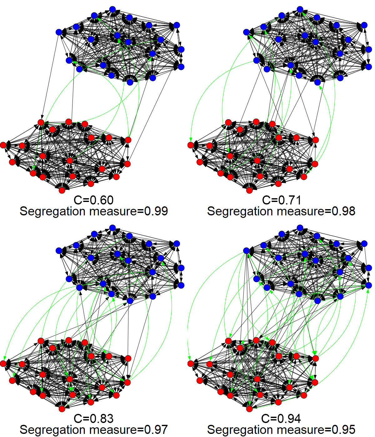
We use the segregation measure defined in (1) as a quantitative measurement of segregation. Networks with high segregation measure have dense intra-community connections but sparse inter-community connections. Fig. 6 shows that segregation measure decreases with higher acceptance probability values, which agrees with our observation of the network structure.
The results indicate that, during polarizing events when users tend to be more segregated, the network administrator can mitigate segregation by spending more efforts on friend recommendations (i.e., to achieve a higher acceptance probability ) so that more inter-community edges can be formed. The results prove ARM’s capability under different social settings.

5.3 Validation of ARM in Opinion Dynamics Model
To verify the efficacy of ARM in mitigating segregation, we implement it on the opinion dynamics model proposed in [14]. In the model, there are two opinions that agents can adopt and express. More precisely, an agent can adopt . The model also accounts for how confident is about the two opinions by two real-valued terms and . At each step, an agent (say ) is chosen at random and expresses its opinion to a randomly chosen neighbor , and responds to ’s expression with agreement or disagreement depending on . The represents an internal evaluation of the opinions based on the social response obtains on expressing them. The value is updated as
| (19) |
where
| (20) |
leading to a positive feedback for and to a negative one if . The parameter represents learning rate.
We incorporate ARM into this model as follows. When agent ’s expression is disagreed by , will be recommended to connect with ’s neighbors who share the same opinion with . Similar to ARM, the recommendation will be accepted with an acceptance probability . Therefore although experiences disagreement with , it will gain some confidence in its expression through agreement with ’s neighbors. The is updated as
| (21) |
where
| (22) |
We use the parameters provided by the authors777See Section 3.2 [14] for implementation details.. The network is a random geometric graph with neighborhood radius . There are agents. take random initial values in . The learning rate . Follow the authors’ implementation, we also set an exploration rate , which measures the probability that agents express their less favorable opinions. We set the recommendation acceptance probability .

As shown in Fig. 7, when agents follow the opinion dynamics model without ARM, the segregation measure of the network keeps increasing and maintains at a high level in the final stage, whereas the segregation measure remains at a relatively low level when agents follow the model is incorporated with ARM. Fig. 8 compares the evolution of the network’s community structure. The network is segregated into nearly disconnected components when ARM is not incorporated. On the contrary, the network is less segregated when ARM is incorporated. This numerical validation in opinion dynamics model verifies the efficacy of ARM in mitigating network segregation.

6 Conclusions and Extensions
Conclusions: This paper considered an edge formation protocol on social networks represented by a directed stochastic block model (DiSBM) to describe how users choose to connect with each other. The edge formation protocol represents how each individual chooses the connection probabilities in order to maximize a utility function that represents the tradeoff between homophily (preference to be connected with one’s own group) and popularity in the different community. Analysis of the game that corresponds to the best response based protocol shows that segregation is the unique Nash equilibrium. We then proposed an algorithmic recommendation mechanism (ARM) to mitigate segregation. ARM recommends users from different communities to form weak ties and provides incentives to those that form them. Assuming each recommendation suggested by the ARM is accepted with an acceptance probability, we show that the segregation level at the Nash equilibrium of the corresponding game depends on it. Thus, the segregation of the network can be controlled by introducing the ARM. We further extend our results to the case where the acceptance probability itself has Markovian dynamics and illustrate how the individuals in the network reach the time-evolving Nash equilibrium of the resulting game. Thus, our results provide a novel mechanism design perspective into the problem of mitigating segregation in social networks.
Limitations and Extensions: The proposed edge formation game and its analysis can be extended to further contexts in several directions.
-
1)
The edge formation protocol proposed in this paper assumes homogeneity among users in one community, i.e., users’ community information solely determines their edge formation probabilities. An interesting future direction is to incorporate heterogeneity (e.g., preferential attachment with fitness) into the network model and apply methods such as friendship paradox sampling [34, 35, 36] to assign different weights to the 2 hop connections between different pairs of users.
-
2)
Another interesting direction is to consider ARM’s parameter (e.g., the recommendation acceptance probability) depends on users’ actions and incorporates a feedback law, i.e., ARM raises the acceptance probability when users become more segregated in network. Such extensions might be helpful in analyzing the existence of Markov Perfect Equilibrium (MPE) of the corresponding stochastic game, which enhances the understanding of users’ long-term strategy in an evolving social network.
- 3)
Appendix A Proofs of Theorems
A.1 Proof of Theorem 1
In Protocol 1, the utility function (2) of each user in the same community is a random variable with the probability distribution induced by the DiSBM model, which has the same expected value. Users in the same community can be viewed as independent copies of a single player. Thus the edge formation game can be reduced to a two-player game, where each player represents users in one community. The utility of the two players, and , are respectively the expected value of the utility function (2) for red and blue users:
| (23) |
| (24) |
It is shown from (23) that is red player’s strictly dominant strategy. This is equivalent to say, at red player’s turn, it will choose as its best response strategy regardless of blue player’s previous action, and will never switch again. Similar result holds for blue player. Therefore the game converges in 2 time steps, i.e., for all .
Thus, the game corresponding to Protocol 1 converges to its unique Nash equilibrium after each player acted once, i.e., users only form intra-community edges and the social network is segregated into echo chambers after .
A.2 Proof of Theorem 2
Similar to the proof of Theorem 1, we assume users in one community are independent copies of a single player and reduce the game with ARM to a two-player game. Based on (11), the utility of the red player and blue player in the two-player game are respectively:
|
|
(25) |
|
|
(26) |
A detailed derivation can be found in Appendix B.
The second order mixed derivatives of (25, 26) yields
| (27) |
Since , the game is submodular, which guarantees that players’ best response strategies converge to a Nash equilibrium [41]. This submodular game also has quadratic utility, which makes it similar to the Bertrand game [12] and thus can be analyzed in a similar approach.
Note that
| (28) |
| (29) |
We apply iterated strict dominance to attain the Nash equilibrium. Let red player’s initial best response set .
-
1)
If , then any is strictly dominated.
-
2)
If , then any is strictly dominated.
The following analysis depends on two different cases of the acceptance probability .
-
1)
If , then , i.e., holds for red player’s possible actions . Thus red player’s best response is
(30) Similarly, blue player’s best response is
(31) Therefore, the Nash equilibrium of the game is
(32) i.e., the social network is in segregation.
-
2)
If , then . Thus, after one iteration, red player’s remaining undominated strategy set, i.e, the best response set is .
Let the set after iterations be , where
(33) (34) We can show that
(35) Therefore, by iteratively applying the best responses and eliminating strictly dominated strategies, the best response strategy converges to the unique Nash equilibrium of the game, which is
(36) The Nash equilibrium () indicates that ARM incentivizes both red and blue users to form inter-community edges, leading to social integration.
A.3 Proof of Theorem 3
Following the proof of Theorem 1 and 2, we assume users in one community are independent copies of a single player and reduce the game to a two-player game. We define the two-player stochastic game resulting from Protocol 3 as follows:
-
1)
A state of the game, , representing the acceptance probability at time .
-
2)
Actions of red player and blue player , , representing their best response strategies at time .
- 3)
-
4)
A transition rule of specified in (16), which is conditionally independent of players’ actions.
-
5)
A discount factor .
-
6)
Value functions of red player and blue player representing their discounted sum of payoff from time
(39) (40)
Based on the above definition of the stochastic game, we aim to derive the player’s optimal strategy under the condition that the acceptance probability evolves as a semi-Markov process. Recall that in Protocol 2 where the acceptance probability is fixed, (in the proof of Theorem 2) we have illustrated the convergence of players’ best response dynamics to the steady state corresponding to the game’s Nash equilibrium. Considering that the state holding time (defined in (16)) is large compared with the time that players take action, we claim that in Protocol 3, players’ best response dynamics converges to the Nash equilibrium corresponding to before it transits.
With this claim, what remains to be proved is how players adapt their actions when transits. Below we illustrate players’ strategy at when transits to another state .
Bellman’s dynamic programming recursion yields [42]:
| (41) |
In (41), and denotes the red user’s value function at time and respectively, assuming that it took the best response at time , which corresponds to the Nash equilibrium of the game with .
The transition dynamics of are conditionally independent of players’ actions. Only the first term in (41), i.e., the one-stage payoff , depends on players’ actions. Thus red player’s optimal strategy is to myopically maximize the one-stage payoff without concerning about the transition of . Similar result holds for blue player’s optimal strategy. Based on the Nash equilibrium (36) derived in Sec. 3.3, are the optimal strategies for red and blue users. Thus, players’ best response dynamics will converge to , i.e., they will reach the time-evolving Nash equilibrium in the resulting game.
Appendix B Derivation of User’s Expected Utility with ARM in Equation (25, 26)
Take red user as an example. The expected number of inter-community edges formed by ARM for any red user is
|
|
(42) |
where denotes expectation over the probability distribution induced by the DiSBM.
On the second line of (42), is the acceptance probability, is the number of blue users, is the probability that the recommendation target has not followed yet, is the probability that is recommended by ARM to any blue user. The third line satisfies when is large, i.e., .
Similarly, ’s expected reward for connecting users from two communities (e.g. a red user connects its red followers to its blue friends) during ARM recommendations is
| (43) |
Acknowledgments
This research was supported in part by the U. S. Army Research Office under grants W911NF-21-1-0093 and W911NF-19-1-0365.
References
- [1] M. McPherson, L. Smith-Lovin, and J. M. Cook, “Birds of a feather: Homophily in social networks,” Annual review of sociology, vol. 27, no. 1, pp. 415–444, 2001.
- [2] C. Musco, C. Musco, and C. E. Tsourakakis, “Minimizing polarization and disagreement in social networks,” in Proceedings of the 2018 World Wide Web Conference, 2018, pp. 369–378.
- [3] M. Cinelli, G. D. F. Morales, A. Galeazzi, W. Quattrociocchi, and M. Starnini, “The echo chamber effect on social media,” Proceedings of the National Academy of Sciences, vol. 118, no. 9, 2021.
- [4] G. Tóth, J. Wachs, R. Di Clemente, Á. Jakobi, B. Ságvári, J. Kertész, and B. Lengyel, “Inequality is rising where social network segregation interacts with urban topology,” Nature communications, vol. 12, no. 1, pp. 1–9, 2021.
- [5] Y. Ge, S. Zhao, H. Zhou, C. Pei, F. Sun, W. Ou, and Y. Zhang, “Understanding echo chambers in e-commerce recommender systems,” in Proceedings of the 43rd International ACM SIGIR Conference on Research and Development in Information Retrieval, 2020, pp. 2261–2270.
- [6] K. Sasahara, W. Chen, H. Peng, G. L. Ciampaglia, A. Flammini, and F. Menczer, “On the inevitability of online echo chambers,” arXiv preprint arXiv:1905.03919, 2019.
- [7] A. Rodriguez-Moral and M. Vorsatz, “An overview of the measurement of segregation: classical approaches and social network analysis,” Complex networks and dynamics, pp. 93–119, 2016.
- [8] R. Luo, B. Nettasinghe, and V. Krishnamurthy, “Echo chambers and segregation in social networks: Markov bridge models and estimation,” IEEE Transactions on Computational Social Systems, 2021.
- [9] V. D. Blondel, J.-L. Guillaume, R. Lambiotte, and E. Lefebvre, “Fast unfolding of communities in large networks,” Journal of statistical mechanics: theory and experiment, vol. 2008, no. 10, p. P10008, 2008.
- [10] M. S. Granovetter, “The strength of weak ties,” American journal of sociology, vol. 78, no. 6, pp. 1360–1380, 1973.
- [11] M. Wilinski, P. Mazzarisi, D. Tantari, and F. Lillo, “Detectability of macroscopic structures in directed asymmetric stochastic block model,” Physical Review E, vol. 99, no. 4, p. 042310, 2019.
- [12] P. Milgrom and J. Roberts, “Rationalizability, learning, and equilibrium in games with strategic complementarities,” Econometrica: Journal of the Econometric Society, pp. 1255–1277, 1990.
- [13] F. Baumann, P. Lorenz-Spreen, I. M. Sokolov, and M. Starnini, “Modeling echo chambers and polarization dynamics in social networks,” Physical Review Letters, vol. 124, no. 4, p. 048301, 2020.
- [14] S. Banisch and E. Olbrich, “Opinion polarization by learning from social feedback,” The Journal of Mathematical Sociology, vol. 43, no. 2, pp. 76–103, 2019.
- [15] C. Blex and T. Yasseri, “Positive algorithmic bias cannot stop fragmentation in homophilic networks,” The Journal of Mathematical Sociology, pp. 1–18, 2020.
- [16] P. R. Neary, “Competing conventions,” Games and Economic Behavior, vol. 76, no. 1, pp. 301–328, 2012.
- [17] M. O. Jackson and A. Wolinsky, “A strategic model of social and economic networks,” Journal of economic theory, vol. 71, no. 1, pp. 44–74, 1996.
- [18] Y. Bramoullé, D. López-Pintado, S. Goyal, and F. Vega-Redondo, “Network formation and anti-coordination games,” international Journal of game Theory, vol. 33, no. 1, pp. 1–19, 2004.
- [19] C. Avin, A. Cohen, P. Fraigniaud, Z. Lotker, and D. Peleg, “Preferential attachment as a unique equilibrium,” in Proceedings of the 2018 World Wide Web Conference, 2018, pp. 559–568.
- [20] N. Alon, M. Feldman, A. D. Procaccia, and M. Tennenholtz, “A note on competitive diffusion through social networks,” Information Processing Letters, vol. 110, no. 6, pp. 221–225, 2010.
- [21] A. Mele, “A structural model of dense network formation,” Econometrica, vol. 85, no. 3, pp. 825–850, 2017.
- [22] Y. Zhang, C. Yang, K. Huang, C. Zhou, and Y. Li, “Robust structure identification of industrial cyber-physical system from sparse data: A network science perspective,” IEEE Transactions on Automation Science and Engineering, 2021.
- [23] Z. Song, H. Guo, D. Jia, M. Perc, X. Li, and Z. Wang, “Third party interventions mitigate conflicts on interdependent networks,” Applied Mathematics and Computation, vol. 403, p. 126178, 2021.
- [24] H.-J. Li, Q. Wang, S. Liu, and J. Hu, “Exploring the trust management mechanism in self-organizing complex network based on game theory,” Physica A: Statistical Mechanics and its Applications, vol. 542, p. 123514, 2020.
- [25] W. Liu, A. Sidhu, A. M. Beacom, and T. W. Valente, “Social network theory,” The international encyclopedia of media effects, pp. 1–12, 2017.
- [26] Y. J. Wang and G. Y. Wong, “Stochastic blockmodels for directed graphs,” Journal of the American Statistical Association, vol. 82, no. 397, pp. 8–19, 1987.
- [27] M. Conover, J. Ratkiewicz, M. Francisco, B. Gonçalves, F. Menczer, and A. Flammini, “Political polarization on twitter,” in Proceedings of the International AAAI Conference on Web and Social Media, vol. 5, no. 1, 2011.
- [28] C. Avin, H. Daltrophe, Z. Lotker, and D. Peleg, “Assortative mixing equilibria in social network games,” in International Conference on Game Theory for Networks. Springer, 2017, pp. 29–39.
- [29] R. Angles and C. Gutierrez, “Survey of graph database models,” ACM Computing Surveys (CSUR), vol. 40, no. 1, pp. 1–39, 2008.
- [30] J. de Marti and Y. Zenou, “Ethnic identity and social distance,” CEPR discussion paper 7566, Tech. Rep., 2009.
- [31] D. Naskar, E. Onaindia, M. Rebollo, and S. Das, “Modelling emotion dynamics on twitter via hidden markov model,” in Proceedings of the 21st International Conference on Information Integration and Web-based Applications & Services, 2019, pp. 245–249.
- [32] A. Iyengar, T. Finin, and A. Joshi, “Content-based prediction of temporal boundaries for events in twitter,” in 2011 IEEE Third International Conference on Privacy, Security, Risk and Trust and 2011 IEEE Third International Conference on Social Computing. IEEE, 2011, pp. 186–191.
- [33] T. Sakaki, M. Okazaki, and Y. Matsuo, “Earthquake shakes twitter users: real-time event detection by social sensors,” in Proceedings of the 19th international conference on World wide web, 2010, pp. 851–860.
- [34] B. Nettasinghe and V. Krishnamurthy, “The friendship paradox: Implications in statistical inference of social networks,” in 2019 IEEE 29th International Workshop on Machine Learning for Signal Processing (MLSP). IEEE, 2019, pp. 1–6.
- [35] ——, “Maximum likelihood estimation of power-law degree distributions using friendship paradox based sampling,” arXiv preprint arXiv:1908.00310, 2019.
- [36] V. Krishnamurthy and B. Nettasinghe, “Information diffusion in social networks: friendship paradox based models and statistical inference,” in Modeling, Stochastic Control, Optimization, and Applications. Springer, 2019, pp. 369–406.
- [37] H.-J. Li, J. Zhang, Z.-P. Liu, L. Chen, and X.-S. Zhang, “Identifying overlapping communities in social networks using multi-scale local information expansion,” The European Physical Journal B, vol. 85, no. 6, pp. 1–9, 2012.
- [38] H.-J. Li, Z. Bu, Z. Wang, and J. Cao, “Dynamical clustering in electronic commerce systems via optimization and leadership expansion,” IEEE Transactions on Industrial Informatics, vol. 16, no. 8, pp. 5327–5334, 2019.
- [39] H.-J. Li, L. Wang, Y. Zhang, and M. Perc, “Optimization of identifiability for efficient community detection,” New Journal of Physics, vol. 22, no. 6, p. 063035, 2020.
- [40] H.-J. Li, Z. Wang, J. Pei, J. Cao, and Y. Shi, “Optimal estimation of low-rank factors via feature level data fusion of multiplex signal systems,” IEEE Transactions on Knowledge and Data Engineering, 2020.
- [41] R. Amir, “Supermodularity and complementarity in economics: An elementary survey,” Southern Economic Journal, pp. 636–660, 2005.
- [42] V. Krishnamurthy, Partially observed Markov decision processes. Cambridge university press, 2016.