Controlling identical linear multi-agent systems over directed graphs

We can distinguish two main cases: either the Laplacian eigenvalues are all real or at least one of them is complex. In the former case, conditions (5a) can be framed within an LMI formulation, through a procedure similar to the one we describe next. In the latter case, we refer to expression (5c), where the problem is lifted to a higher space, considering $A_{e,k}$ instead of $A_{k}$, so as to work with real-valued matrices. We focus on the latter case, which is more general and includes the former. Let us define the inverse of $P_{e,k}$ in (5c)

with $Q_{k}$ symmetric positive definite and $\Sigma_{k}$ skew-symmetric. In fact, $Q_{k}^{-1}=P_{k}-\Pi_{k}^{\top}P_{k}^{-1}\Pi_{k}$ (which is invertible, since applying the Schur complement to $P_{e,k}$ yields $Q_{k}^{-1}\succ 0$) and $\Sigma_{k}=P_{k}^{-1}\Pi_{k}Q_{k}=Q_{k}\Pi_{k}P_{k}^{-1}$ (where the equality holds because $\Pi_{k}P_{k}^{-1}Q_{k}^{-1}=\Pi_{k}-\Pi_{k}P_{k}^{-1}\Pi_{k}^{\top}P_{k}^{-1}\Pi_{k}=(P_{k}-\Pi_{k}P_{k}^{-1}\Pi_{k}^{\top})P_{k}^{-1}\Pi_{k}=Q_{k}^{-1}P_{k}^{-1}\Pi_{k}$ ). Then, we can left- and right- multiply inequality (5c) by $Q_{e,k}$, obtaining

To look for a common state-feedback matrix $K$, even when the matrices $Q_{e,k}$ are different, we take advantage of the results in [16]. We can rewrite (6) as

where $\Phi_{\mu}=\left[\begin{smallmatrix}2\mu&1\\ 1&0\end{smallmatrix}\right]$ describes the stability region, which in our case is the complex half-plane with real part smaller than $-\mu$. Then, according to [16, Section 3.1], (7) is equivalent to the existence of matrices $X_{1,k},X_{2,k}\in{\mathbb{R}}^{2n\times 2n}$ satisfying

where $X_{1,k}$ and $X_{2,k}$ are multipliers that add degrees of freedom by decoupling matrices $Q_{e,k}$ and $A_{e,k}$. Conditions (8) are still necessary and sufficient for $\mu$–synchronization, because they are equivalent to (7).

According to the derivation in [16, Section 3.3], imposing ${X_{2,k}}=\alpha{X_{1,k}}$, with $\alpha>0$, does not add conservatism as far as there are $\nu$ independent matrices ${X_{1,k}}$. We are now going to relax this condition by assuming that matrices $X_{1,k}$ and $X_{2,k}$ have the specific structure

where $X_{e}:=\left[\begin{smallmatrix}X&0\\ 0&X\end{smallmatrix}\right]=I_{2}\otimes X$, with $X\in{\mathbb{R}}^{n\times n}$, is a block-diagonal matrix common to all $\nu$ inequalities, while $Z_{k},W_{k}\in{\mathbb{R}}^{2n\times 2n}$ are different multipliers for every inequality. This assumption introduces conservativeness; therefore, the conditions are now only sufficient. However, we can now expand (8) and obtain the bilinear formulation

with ${\Theta_{k}}=\bigl{(}I_{2}\otimes AX\bigr{)}-\bigl{(}\Lambda_{k}\otimes B{Y}\bigr{)}$, where $\Lambda_{k}=\left[\begin{smallmatrix}\alpha_{k}&-\beta_{k}\\ \beta_{k}&\alpha_{k}\end{smallmatrix}\right]$ is related to the $k$-th eigenvalue $\lambda_{k}=\alpha_{k}+\jmath\beta_{k}$ and $Y:=KX$ is a suitable change of variables. An expanded version of (9) with the variables highlighted is provided in equation (12) at the top of the next page.

Constraints (9) alone, might lead to badly conditioned optimized selections of $K$, due to the fact that the joint spectral abscissa of $A_{e,k}$ for all $k=1,\ldots,\nu$ may potentially grow unbounded for arbitrarily large values of $K$. Thus, as a possible sample formulation of a multi-objective optimization, we fix a maximum desired norm $\bar{\kappa}$ for $K$ and enforce the constraint $\|K\|\leq{\bar{\kappa}}$ through the following LMI formulation:

stemming from the expression $K^{\top}K\preceq{{\bar{\kappa}}}^{2}I$ after applying a Schur complement and exploiting $(X-I)(X^{\top}-I)\succeq 0$.

We then suggest to synthesize a state-feedback matrix $K$ satisfying $\|K\|\leq{\bar{\kappa}}$ and maximizing $\mu$ by solving the bilinear optimization problem

where alternative performance-oriented linear constraints can be straightforwardly included, and then selecting $K=YX^{-1}$. An iterative approach can be used to make the problem quasi-convex and solve it iteratively with standard LMI techniques.

In order to solve the BMI optimization problem (11) with convex techniques, we focus our attention on BMI (9), since the other constraints are linear, and we propose an iterative approach for the problem solution, described in Algorithm 1. The algorithm is composed of two steps:
1) Synthesis step: for given fixed multipliers $Z_{k}$ and $W_{k}$, $k=1,\ldots,\nu$, optimization (11) is solved in the decision variables $(\mu,X,Y,Q_{e,k})$, which corresponds to a generalized eigenvalue problem (easily solvable by a bisection algorithm) due to the fact that matrices $Q_{e,k}$ are all positive definite;
2) Analysis step: for given fixed matrices $X$ and $Y$, optimization (11) is solved in the decision variables $(\mu,Z_{k},W_{k},Q_{e,k})$, which corresponds again to a generalized eigenvalue problem due to positive definiteness of $Q_{e,k}$.

Algorithm 1 essentially comprises iterations of the two steps above, until parameter $\mu$ increases less than a specified tolerance over two steps. To the end of establishing a useful means of comparison in the simulations reported in Section IV, we naively initialize the algorithm by fixing the initial multipliers as scaled identity matrices (with $\alpha>0$ properly tuned). More generally, we emphasize that using the Riccati construction of [10], stabilizability of $(A,B)$ is sufficient for ensuring the existence of a Riccati-based solution of (11) and it is immediate to design an infinite gain margin solution where all the matrices $A_{e,k}$ share a common quadratic Lyapunov function. We do not pursue this initialization here, so as to perform a fair comparison between our algorithm (initialized in a somewhat naive way) and the construction resulting from [10].

The following proposition establishes useful properties of the algorithm.

In our simulations we consider two types of agent dynamics: one is oscillatory,

while the second one is the unstable lateral dynamics of a forward-swept wing, the Grumman X-29A, as in [14],

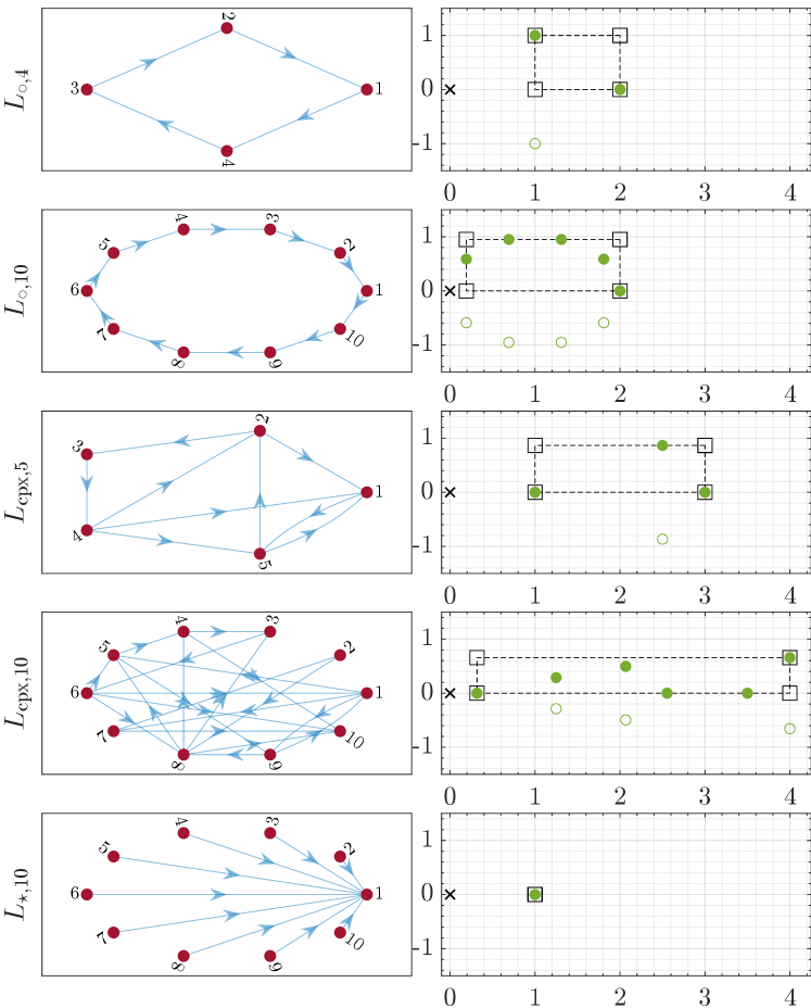
We consider five communication networks: two circular graphs with $N=4$ and $N=10$ agents, two generic directed graphs with $N=5$ and $N=10$ agents characterized by complex eigenvalues, and a star graph with $N=10$ agents. The graph topologies and the eigenvalues of the associated Laplacian matrices are visualized in Fig. 1.

The approaches that we compare are the following ones:

1. a.

   [Riccati], the dual case of [10, Section 5.5]: the gain is structured as $K=B^{\top}P$, where $P$ is the unique solution to the algebraic Riccati equation

   $$A^{\top}P+PA-2bPBB^{\top}P+aI=0,$$

   (13)

   with $b\leq\operatorname{Re}(\lambda_{k})$ and $a>0$. We solve (13) by fixing $b=\min(\operatorname{Re}(\lambda_{k}))$ and adjusting the value of $a$ so as to respect the bound $\|K\|\leq{\bar{\kappa}}$, which is easily done due to the monotonicity of $\|K\|$ with respect to $a$.

2. b.

   [Listmann] from [14]: LMI conditions (6) with $Q_{e,k}=\left[\begin{smallmatrix}Q&0\\ 0&Q\end{smallmatrix}\right]$ and $Y=KQ$ are imposed for the $\lambda_{k}$ corresponding to the corners of a rectangular box in the complex plane that includes all non-zero eigenvalues of $L$ (considering the eigenvalues in the first quadrant is enough, since conjugate eigenvalues lead to the same condition), while incorporating in the LMI-based design the maximum norm condition (10). A fixed number of LMIs need to be solved regardless of the network size.

3. c.

   [$A_{e,k}$]: the method resembles that in “b”, but now conditions (6) are imposed for each $\lambda_{k}$, $k=1,\dots,\nu$.

4. d.

   [Direct]: one iteration of Algorithm 1 is executed, which amounts to solving (11) with $Z_{k}=I_{2n}$, $W_{k}=\alpha I_{2n}$ and $\alpha>0$ properly tuned. Notably, matrices $Q_{e,k}$ do not have a pre-defined structure.

5. e.

   [Algorithm 1]: the procedure in Algorithm 1 is executed up to its termination, as guaranteed by Proposition 2.

In the simulations, the convergence rate of the solutions is estimated from the spectral abscissa of matrices $A_{k}$ in (5a), namely, from the largest-real-part eigenvalue:

We implement the different procedures in MATLAB, using the toolbox YALMIP [17] with MOSEK as an LMI solver. For the algorithm, we consider a tolerance of $10^{-3}$ and ${\bar{\kappa}}=20$ as the bound on the norm of $K$.

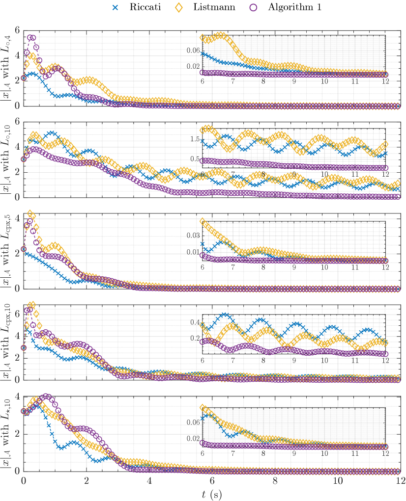
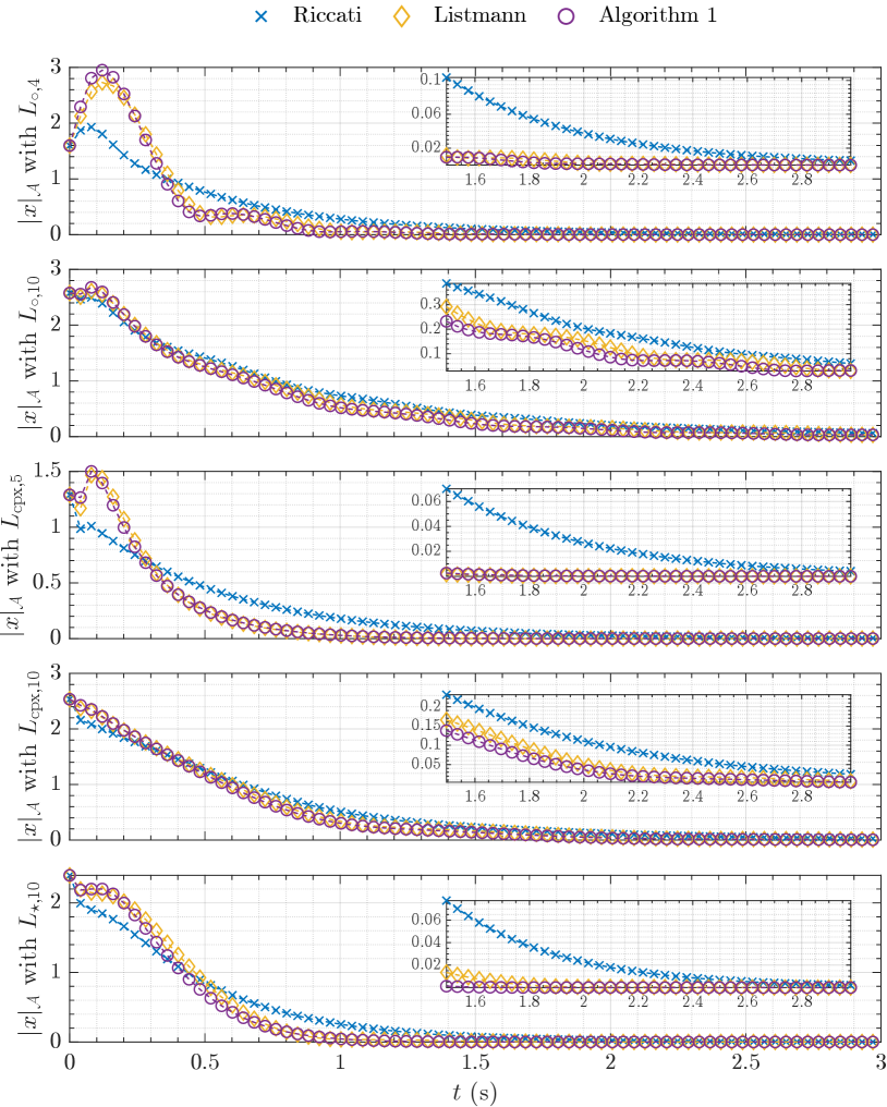
For the different combinations of dynamics and graph topologies, Table I reports a summary of all our results, along with estimated converge rate $\hat{\mu}$, norm of $K$ and execution time. The time evolutions of the distances from the synchronization set $\mathcal{A}$ are shown in Figs. 2 and 3 for the approaches “a”, “b” and “e”.

Generally, method “a” has a worse performance than the considered LMI-based methods. The gain bound is reached, but the convergence rate is the slowest, most likely because the approach is forcing an infinite gain margin for $K$. Locating the eigenvalues of the $A_{k}$ matrices in the complex plane shows that method “a” tends to move to the left a few eigenvalues (faster modes) and penalize others, so that the convergence speed is limited.

Method “b” performs similarly to “c”, as expected, since the two methods simply consider different (eigen)values. In general, method “b” is more conservative than “c”, but is faster in larger networks. With $L_{cpx,5}$ and $L_{cpx,10}$, method “b” is slightly more conservative, as is reasonable, since it considers values that are not in the spectrum of the Laplacian.

Method “d” generally yields better results than “b” and “c”, provided that proper values of the parameter $\alpha$ are chosen. This improvement is due to the decoupling between matrices $A_{e,k}$ and $Q_{e,k}$.

The best results are obtained using our proposed Algorithm 1, which gives the highest convergence rate and gets close to the system specifications. However, the computational load is higher, since several iterations are needed. With dynamics $A_{\text{X-29}}$, the states are always converging faster; with dynamics $A_{\text{osc}}$, the performance is similar to that obtained with other non-iterative LMI-based techniques. Algorithm 1 outperforms the other procedures in the case with dynamics $A_{\text{X-29}}$ and graph $L_{\circ,10}$: even though it requires quite some iterations to converge, it provides a controller that leads to almost one-order-of-magnitude faster convergence than the others, as shown in Fig. 2.

References

- [1] R. Olfati-Saber, J. A. Fax, and R. M. Murray, “Consensus and Cooperation in Networked Multi-Agent Systems,” Proceedings of the IEEE, vol. 95, no. 1, pp. 215–233, 2007.
- [2] L. Scardovi and R. Sepulchre, “Synchronization in networks of identical linear systems,” Automatica, vol. 45, no. 11, pp. 2557–2562, 2009.
- [3] M. Mesbahi and M. Egerstedt, Graph Theoretic Methods in Multiagent Networks. Princeton University Press, 2010.
- [4] F. Xiao and L. Wang, “Consensus problems for high-dimensional multi-agent systems,” IET Control Theory & Applications, vol. 1, no. 3, pp. 830–837, 2007.
- [5] C.-Q. Ma and J.-F. Zhang, “Necessary and Sufficient Conditions for Consensusability of Linear Multi-Agent Systems,” IEEE Transactions on Automatic Control, vol. 55, no. 5, pp. 1263–1268, 2010.
- [6] Z. Li, Z. Duan, G. Chen, and L. Huang, “Consensus of Multiagent Systems and Synchronization of Complex Networks: A Unified Viewpoint,” IEEE Transactions on Circuits and Systems I: Regular Papers, vol. 57, no. 1, pp. 213–224, 2010.
- [7] L. Dal Col, S. Tarbouriech, L. Zaccarian, and M. Kieffer, “A consensus approach to PI gains tuning for quality-fair video delivery,” International Journal of Robust and Nonlinear Control, vol. 27, no. 9, pp. 1547–1565, 2017.
- [8] G. Giordano, I. Queinnec, S. Tarbouriech, L. Zaccarian, and N. Zaupa, “Equivalent conditions for the synchronization of identical linear systems over arbitrary interconnections,” 2023. [Online]. Available: https://arxiv.org/abs/2303.17321
- [9] J. Qin, H. Gao, and W. X. Zheng, “Exponential Synchronization of Complex Networks of Linear Systems and Nonlinear Oscillators: A Unified Analysis,” IEEE Transactions on Neural Networks and Learning Systems, vol. 26, no. 3, pp. 510–521, 2015.
- [10] A. Isidori, Lectures in Feedback Design for Multivariable Systems. Springer International Publishing, 2017, ch. 5.
- [11] F. Bullo, Lectures on Network Systems. Kindle Publishing, 2022, ch. 8.
- [12] A. Saberi, A. A. Stoorvogel, M. Zhang, and P. Sannuti, Synchronization of Multi-Agent Systems in the Presence of Disturbances and Delays. Springer International Publishing, 2022.
- [13] H. L. Trentelman, K. Takaba, and N. Monshizadeh, “Robust Synchronization of Uncertain Linear Multi-Agent Systems,” IEEE Transactions on Automatic Control, vol. 58, no. 6, pp. 1511–1523, 2013.
- [14] K. D. Listmann, “Novel conditions for the synchronization of linear systems,” in 54th IEEE Conference on Decision and Control, 2015.
- [15] S. Boyd, L. El Ghaoui, E. Feron, and V. Balakrishnan, Linear Matrix Inequalities in System and Control Theory. SIAM, 1994.
- [16] G. Pipeleers, B. Demeulenaere, J. Swevers, and L. Vandenberghe, “Extended LMI characterizations for stability and performance of linear systems,” Systems & Control Letters, vol. 58, no. 7, pp. 510–518, 2009.
- [17] J. Löfberg, “Yalmip: A toolbox for modeling and optimization in matlab,” in Proceedings of the CACSD Conference, 2004.