Controlling cell motion and microscale flow with polarized light fields

Natural microswimmers, such as bacteria and algae, can achieve autonomous motion by converting locally stored energy into mechanical work (Lauga and Powers, 2009; Ramaswamy, 2010; Poon, 2013; Aranson, 2013; Wang et al., 2013; Sanchez et al., 2015; Elgeti et al., 2015; Bechinger et al., 2016; Lavrentovich, 2016; Zottl and Stark, 2016; Patteson et al., 2016; Zhang et al., 2017; Illien et al., 2017; Liebchen and Loewen, 2018; Gompper et al., 2020). Such cellular motility is not only an essential aspect of life but also an inspirational source to develop artificial microswimmers, which propel themselves through self-generated fields of temperature, chemical concentration, or electric potential (Lauga and Powers, 2009; Poon, 2013; Aranson, 2013; Wang et al., 2013; Sanchez et al., 2015; Elgeti et al., 2015; Zhang et al., 2017; Illien et al., 2017). Both natural and artificial microswimmers have been used in a wide variety of applications (Wang, 2012; Gao and Wang, 2014; Li et al., 2017; Alapan et al., 2019).

To properly function in a fluctuating heterogeneous environment, microswimmers need to adjust their motility in response to external stimuli (Menzel, 2015; Stark, 2016; You et al., 2018; Klumpp et al., 2019). For example, intensity and direction of ambient light can induce a variety of motility responses in photosynthetic microorganisms (Mikolajczyk et al., 1990; Jekely, 2009; Drescher et al., 2010; Barsanti et al., 2012; Kane et al., 2013; Garcia et al., 2013; Giometto et al., 2015; Bennett and Golestanian, 2015; Chau et al., 2017; Hader and Iseki, 2017; Ozasa et al., 2017; Arrieta et al., 2017; Tsang et al., 2018; Arrieta et al., 2019; Choudhary et al., 2019) and artificial microwimmers (Xu et al., 2017; Dong et al., 2018; Wang et al., 2018; Aubret et al., 2018; Singh et al., 2018; Zhan et al., 2019; Lavergne et al., 2019); these responses have been frequently used to control microswimmer motion (Arlt et al., 2018; Tsang et al., 2018; Arrieta et al., 2017; Dervaux et al., 2017; Ogawa et al., 2016; Stenhammar et al., 2016; Palacci et al., 2013; Frangipane et al., 2018; Ozasa et al., 2017; Lozano et al., 2016; Giometto et al., 2015; Geiseler et al., 2016; Barsanti et al., 2012; Lavergne et al., 2019). Besides intensity and direction, light polarization can also affect microswimmer motility and lead to polarotaxis: Euglena gracilis cells align their motion direction perpendicular to the light polarization, possibly to maximize the light absorption (CREUTZ and DIEHN, 1976; Hader, 1987); artificial microswimmers consisting of two dichroic nanomotors move in the polarization direction (Zhan et al., 2019). These previous experiments have focused on uniform light fields (CREUTZ and DIEHN, 1976; Hader, 1987; Zhan et al., 2019). The possibility to use complex polarization patterns to control polarotactic microswimmers has not been explored.

In this letter, we investigate Euglena gracilis cell motion in various polarized light fields in a quantitative and systematic fashion. Our experiments show that while spatially uniform polarization aligns cells into a global nematic state with no net motion, spatially varying fields can induce both local nematic order and mean cell motion. Further, we show that ordered cell swimming motion generates fluid flow that can transport passive tracers. Using the experimental data of individual cells, we construct a model to describe the influence of local light polarization on cell orientation dynamics and quantitatively reproduce all experimental observations.

Experiments - Euglena gracilis are unicellular flagellated microorganisms with a rod-shaped body of a length $\sim$ 50 $\mu$m and a width $\sim$ 5 $\mu$m. As shown in Fig. 1(a) and Movie S1 in the Supplemental Material (APS, 2020), cells swim at a mean speed $\sim$ 60 $\mu$m/s (with a standard deviation of $10\text{ }\mu$m/s.), while rolling around their long axis at a frequency of 1-2 Hz (Rossi et al., 2017). A photoreceptor on Euglena cell surface, marked as a red dot in Fig. 1(b), senses surrounding light and generate signals to modulate flagellar beating pattern (Hill and PLUMPTON, 2000; Hader and Iseki, 2017).

In our experiments, Euglena culture is sealed in a disk-shaped chamber ($\sim 150\text{ }\mu$m in thickness and 24 mm in diameter), which is placed in an illuminating light path, as shown in Fig. S1 (APS, 2020). A collimated blue light beam is used to excite cell photo-responses; the default light intensity is 100 $\mu\text{W/cm}^{2}$. Various polarized optical fields can be generated by using different birefringent liquid crystal plates and by changing relative angles between optical elements (Delaney et al., 2017). Cell motion is recorded by a camera mounted on a Macro-lens. Default system cell density ( $\rho_{0}=$ 8 cells/mm² ) is sufficiently low that we can use a standard particle tracking algorithm (Zhang et al., 2010) to measure position, orientation, and velocity of cells. The current work mainly focuses on steady state dynamics that is invariant over time.

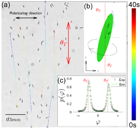
Uniformly polarized light field - Euglena photoreceptor contains dichroically oriented chromoproteins which lead to polarization-dependent photo responses (BOUND and TOLLIN, 1967; CREUTZ and DIEHN, 1976; Hader, 1987; Hader and Iseki, 2017). As shown in Fig. 1(a), cells in a horizontally polarized field tend to orient and swim perpendicularly to the polarization (CREUTZ and DIEHN, 1976); we denote such a targeted direction for cells as $\theta_{T}$. Quantitatively, we measure the $j$th cell’s location $\vec{r}_{j}\left(t\right)$, velocity $\vec{v}_{j}$, and velocity angle $\varphi_{j}$, cf. Fig. 1(b). Over a square window (1.2 mm²), we define mean cell velocity as $\vec{v}=\left\langle\vec{v}_{j}\right\rangle$, where average $\left\langle\cdot\right\rangle$ runs over all cells in the region during the measurement time; nematic order parameter and orientation angle are defined as $u=\text{$\left|\left\langle\exp\left(\text{i}\left(2\varphi_{j}\right)\right)\right\rangle\right|$}$ and $\phi_{u}=\frac{1}{2}\text{Arg}\left(\left\langle\exp\left(\text{i}\left(2\varphi_{j}\right)\right)\right\rangle\right)$, where Arg denotes the phase angle of a complex number. In uniform fields, cells are homogeneously distributed over space and form a global nematic state with a vanishing mean cell velocity: $u\approx 0.75$ and $\vec{v}\approx 0$.

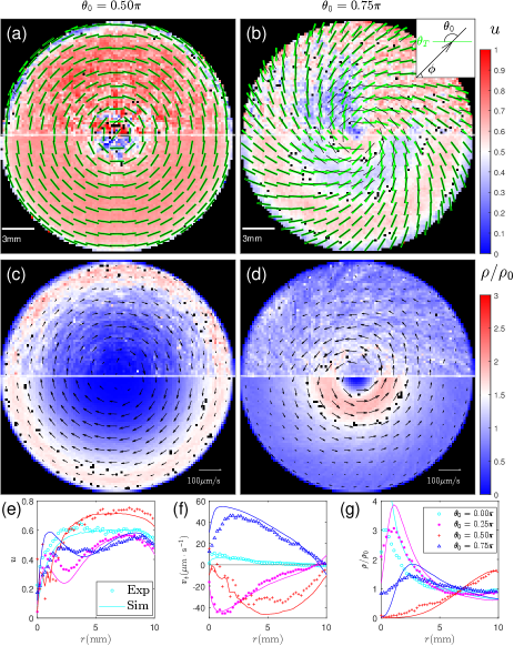
Axisymmetric light field - We next investigate cell motion in light fields with spatially varying polarization. In our experiments, the targeted direction field $\theta_{T}\left(\vec{r}\right)$ is designed to have the form of $\theta_{T}\left(\vec{r}\right)=k\phi\left(\vec{r}\right)+\theta_{0}$, where $k$ is a winding number, $\phi=\tan^{-1}\left(y/x\right)$ is the polar angle, and $\theta_{0}$ is a spiral angle (cf. inset of Fig. 2(b)). When $k=1$, $\theta_{T}\left(\vec{r}\right)$ field is axisymmetric as shown by short green lines in Fig. 2 (a-b) and $\theta_{0}$ controls the ratio between bend and splay strength.

Cell motion in axisymmetric fields can be seen in Movies S2-S5 (APS, 2020). Quantitatively, mean nematic order parameter, cell velocity, and cell density are plotted in Fig. 2 and Fig. S3 (APS, 2020). As shown in Fig. 2(e), nematic order parameter $u$ increases from the defect center to the exterior of the illuminated region, where spatial gradients of $\theta_{T}\left(\vec{r}\right)$ are small and cells closely follow $\theta_{T}\left(\vec{r}\right)$. Cells in pure bend ($\theta_{0}=\pi/2$) and mixed ($\theta_{0}=3\pi/4$) light fields also exhibit mean velocity; peak value in radial profiles in Fig. 2(f) is about $50\text{ }\mu$m/s. Spatial distributions of cells depend on $\theta_{0}$: while cells aggregate at the exterior boundary for $\theta_{0}=\pi/2$, Fig. 2(g) shows a relatively flat distribution with a small peak at $r=2.6$ mm for $\theta_{0}=3\pi/4$ and cell aggregation near the defect center for other two $\theta_{0}$ conditions. We also systematically vary light intensity and system cell density; qualitatively similar results are shown in Figs. S4-S5 and Movie S7 in the Supplemental Material (APS, 2020).

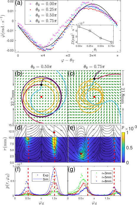
Deterministic model - Fig. 1 and Fig. 2 show that cells tend to align their motion direction $\varphi$ towards the local targeted direction $\theta_{T}\left(\vec{r}\right)$. To quantify this nematic alignment interaction, we extract the time derivative of motion direction $\dot{\varphi}_{j}$ from cell trajectories and find that $\dot{\varphi}_{j}$ is a function of the angular deviation $\varphi_{j}-\theta_{T}\left(\vec{r}_{j}\right)$. We average the dependence function over all cells in a given experiment. Mean $\dot{\varphi}$ in Fig. 3(a) can be adequately described by the following equation:

Fitting data in Fig. 3(a) leads to a nematic interaction strength $A=0.022\text{ rad/s}$ (Li et al., 2019) and a constant angular velocity $C=-0.005\text{ rad/s}$ for default light intensity; parameter $A$ increases with light intensity, and $C$ shows a weak dependence, as shown in Fig. S4(e) (APS, 2020). Small negative $C$ value indicates that cells have a weak preference to swim clockwise; such chirality has been reported before (Tsang et al., 2018) and is likely caused by the symmetry breaking from handedness of cell body rolling and directionality of the illuminating light, cf. Fig. S1 (APS, 2020). This weak chirality explains the non-zero mean cell velocity in an achiral light field in Fig. 2(c) ($\theta_{0}=\pi/2$). To describe cell translational motion in our model, we assume all cells have the same speed $v_{\circ}=60\text{ }\mu$m/s and update cell’s position with a velocity

In axisymmetric fields, particle dynamics from Eqs. (1-2) can be described by two variables: the radial coordinate $r$ and the angular deviation from the local polar angle $\varphi_{d}=\varphi-\phi$. We solve the governing equations for these quantities (cf. the Supplemental Material (APS, 2020)) and compute particle trajectories in $\left(r,\varphi_{d}\right)$ phase plane, as shown dark lines in Fig. 3(d-e). Fixed point in the phase plane is identified at $r^{*}=\left|\frac{v_{\circ}}{C-A\sin 2\theta_{0}}\right|$ and $\varphi_{d}^{*}=\frac{\pi}{2}$ (if $C>A\sin 2\theta_{0}$) or $\varphi_{d}^{*}=-\frac{\pi}{2}$ (if $C<A\sin 2\theta_{0}$); it is stable if $\cos 2\theta_{0}<0$, neutrally stable if $\cos 2\theta_{0}=0$, and unstable if $\cos 2\theta_{0}>0$. At stable and neutrally stable fixed points, particle moves along circular trajectories, cf. the violet trajectory in Fig. 3(b). Around neutrally stable fixed points, there is a family of closed trajectories in $\left(r,\varphi_{d}\right)$ phase plane; in real space, such trajectories appear to be processing ellipses around the defect center, cf. yellow trajectories in Fig. 3(c) and Fig. S8(c) (APS, 2020).

Langevin model - Cell motion contains inherent noises, which may arise from flagellum dynamics or cell-cell interactions. To account for this stochasticity, we add a rotational noise term $\sqrt{2D}\xi\left(t\right)$ to Eq. (1), which becomes Eq. (S1) (APS, 2020); $\xi\left(t\right)$ represents Gaussian white noise with zero-mean $\left\langle\xi\left(t\right)\xi\left(0\right)\right\rangle=\delta\left(t\right)$ and $D$ is an effective rotational diffusivity. With this noise term, Eq. (S1) and Eq. (2) constitute a Langevin model of an active Brownian particle whose orientation is locally modulated by the light polarization, i.e. $\theta_{T}$. The corresponding Fokker-Planck equation can be written down for the steady-state probability density, $p\left(\vec{r},\varphi\right)$, of finding a particle at a state $\left(\vec{r},\varphi\right)$. For uniformly polarized field, the probability distribution $p\left(\varphi\right)$ can be analytically solved and fitted to data in Fig. 1(c), yielding an estimation of $D/A=0.17\text{\text{ }rad}$ for this experiment.

We then consider axisymmetric fields. Probability density $p\left(r,\varphi_{d}\right)$ is experimentally measured and Fig. 3 (d-e) show high value around stable/neutrally stable fixed points. This highlights the importance of fixed points: their radial positions determine cell distributions in Fig. 2(c-d) and they appear at either $\varphi_{d}^{*}=+\frac{\pi}{2}$ or $\varphi_{d}^{*}=-\frac{\pi}{2}$, which breaks the chiral symmetry and leads to a non-zero mean velocity. $p\left(r,\varphi_{d}\right)$ measured in two other cases of $\theta_{0}$ are shown in Fig. S3 (APS, 2020). To quantitatively reproduce measured $p\left(r,\varphi_{d}\right)$, we numerically integrate the Langevin model: parameters $A$ and $C$ values extracted from Fig. 3(a) are used and the effective angular diffusivity $D$ is tuned to fit experimental measurements, see inset of Fig. 3(a). Our numerical results agree well with experiments for probability density profiles in Fig. 3 (f-g) and for radial profiles in Fig. 2 (e-g).

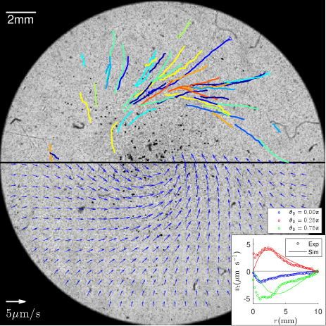
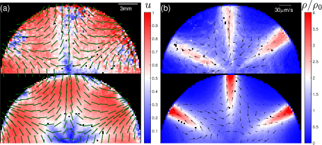
Transport of passive particles - Ordered swimming of Euglena cells in Fig. 2 can collectively generate fluid flow (Mathijssen et al., 2018), which we use hollow glass spheres (50 $\mu$m) on an air-liquid interface to visualize. Tracer trajectories from an experiment are shown in the top half of Fig. 4 and particles spiral counter-clock-wisely towards the center with a peak speed about 5 $\mu$m/s. To compute the generated flow, we represent swimming cells as force-dipoles (Ogawa et al., 2017; Bardfalvy et al., 2020): a dipole in a state $\left(\vec{r},\varphi\right)$ generate flow velocity $\vec{w}\left(\vec{r}_{s};\vec{r},\varphi\right)$ (including contributions from a force-dipole (Ogawa et al., 2017) and its image (Happel and Brenner, 1965; Mathijssen et al., 2015)) at a location on the surface $\vec{r}_{s}$. Then, for a given light field, the Langevin model is used to simulate the motion of $N$ cells and to find the probability distribution of cells $p\left(\vec{r},\varphi\right)$. Finally, we compute the total flow as: $\vec{W}\left(\vec{r}_{s}\right)=N\int p\left(\vec{r},\varphi\right)\vec{w}\left(\vec{r}_{s};\vec{r},\varphi\right)\text{d}\text{$\vec{r}$d$\varphi$}$, see Sec. II(F) in the Supplemental Material (APS, 2020) for details. This approach generates flow fields (cf. bottom half and inset of Fig. 4) that are consistent with measured tracer velocities, see also Fig. S6 (APS, 2020).

Discussion - Our setup can also generate nonaxisymmetric light fields with integer winding numbers. Fig. 5 shows that cells in a $k=-2$ field form dense and outgoing bands in regions where $\theta_{T}$ is close to be radial; these observations can be explained by stable radial particles trajectories in Fig. S9 (also Movie S6) (APS, 2020). The Langevin model is used to investigate light fields with half-integer defects and multiple defects (Rosales-Guzman et al., 2018); results of cell dynamics and transporting flow in Figs. S12 and S13 (APS, 2020) demonstrate that our idea of local orientation modulation can be used as a versatile and modular method for system control.

Local orientation modulation has been previously implemented by embedding rod-shaped bacteria in nematic liquid crystal with patterned molecular orientation (Trivedi et al., 2015; Peng et al., 2016; Aranson, 2018; Turiv et al., 2020; Koizumi et al., 2020). In this bio-composite system, while cell orientation is physically constrained by aligned molecules, bacteria swimming can in return disrupt the molecular order; this strong feedback weakens the controlling ability of the imposed pattern and leads to highly complex dynamics (Trivedi et al., 2015; Peng et al., 2016; Aranson, 2018; Turiv et al., 2020; Koizumi et al., 2020). By contrast, our method relies on biological responses, instead of physical interactions, to achieve orientation control, and Euglena motion has no effect on the underlying light field. Such a one-way interaction leads to a much simpler system and may help us to achieve more accurate control. Furthermore, our method works on cells in their natural environment and requires no elaborate sample preparation. This factor and the spatio-temporal tunability of light fields (Rosales-Guzman et al., 2018) make our method flexible and easy to use.

Sinusoidal term in Eq. (1) is the simplest harmonic for nematic alignment. The same term has been observed in dichroic nano-particle systems (Tong et al., 2010; Zhan et al., 2019) and is related to the angular dependence of dichroic light absorption. These nano-particle systems usually require very strong ($\sim$ $\text{W/cm}^{2}$-$\text{MW/cm}^{2}$ ) light stimulus to operate. By contrast, biological response in Euglena greatly amplifies the light signal and functions in the range of 100 $\mu\text{W/cm}^{2}$; this high sensitivity significantly reduces the complexity to construct a controlling light field.

Conclusion - To summarize, we have experimentally demonstrated that Euglena motion direction is strongly affected by the local light polarization and that cell dynamics in spatially varying polarization fields is controlled by topological properties and light intensity of the underlying fields. Our experiments also showed that ordered cell swimming, controlled by the polarization field, can generate directed transporting fluid flow. Experimental results have been quantitatively reproduced by an active Brownian particle model in which particle motion direction is nematically coupled to the local light polarization; fixed points and closed trajectories in the model have strong impacts on system properties. These results suggest that local orientation modulation, via polarized light or other means, can be used as a general method to control active matter and micro-scale transporting flow.