Control of a spin qubit in a lateral GaAs quantum dot based on symmetry of gating potential
Abstract
We study the influence of quantum dot symmetry on the Rabi frequency and phonon-induced spin relaxation rate in a single-electron GaAs spin qubit.
We find that anisotropic dependence on the magnetic field direction is independent of the choice of the gating potential.
Also, we discover that relative orientation of the quantum dot, with respect to the crystallographic frame,
is relevant in systems with , , or () symmetry.
To demonstrate the important impact of the gating potential shape on the spin qubit lifetime,
we compare the effects of an infinite-wall equilateral triangle,
square, and rectangular confinement with the known results for the harmonic potential.
In the studied cases, enhanced spin qubit lifetime is revealed, reaching almost six
orders of magnitude increase for the equilateral triangle gating.
PACS numbers:
81.07.Ta, 71.70.Ej, 72.10.Di, 76.30.−v, 31.15.Hz
I Introduction
Every quantum two-level system can act as the quantum bit, a basic unit of quantum information processing NC10 ; BdV . Among different solid-state implementations of the qubit system LdV98 ; OTW+99 ; NPT99 ; YTB+12 , single-electron spin in a semiconductor quantum dot (QD) can be used to achieve the task. In order to manipulate spins of charge carriers embedded inside a semiconductor material electrically, through electric dipole spin resonance (EDSR) R60 , the presence of spin-orbit interaction (SOI) is obligatory.
Besides its positive effect in EDSR based schemes GBL06 ; BL07 ; NKN+07 ; R08 ; BSO+11 ; KSW+14 ; TYO+18 ; KLS19 ; SKT+19 , SOI enables the electron-phonon coupling mediated transitions between the qubit states KN00 ; PF05 ; S17 ; LLH+18 , affecting the spin qubit lifetime. To suppress the coupling to phonons, different approaches like the optimization of the QD design CBG+07 ; MSL16 or control of the system size CM07 were suggested. The observed anisotropy of the spin relaxation rate on the in-plane magnetic field orientation FAT05 offered another playground for fine-tuning of the spin qubit’s desired properties. In circular QDs, this is the only degree of freedom accessible in the optimization of the spin qubit, while for the elliptical confining potential SKS+14 ; MSL16 ; OS07 ; AMR+08 orientation of the QD potential with respect to the crystallographic frame can be used as the tuning parameter.
Evidently, different symmetry of the gating potential PRC15 is the main reason for the observed behavior. But to what extent can the potential symmetry alter the basic properties of the electrically controlled spin qubit? To address this question, we have performed a general analysis valid for the lateral GaAs QD system with or symmetry of the gating potential. Besides the expected anisotropy on the magnetic field orientation, we were able to find potential symmetries for which the QD orientation with respect to the crystallographic frame can act as another control parameter of the spin qubit characteristics. With our theory, we offer a simple and efficient way to determine the impact of the gating potential on the Rabi frequency and spin relaxation rate. This is shown in the example of anisotropic and isotropic harmonic potential, as well as for the infinite-wall equilateral triangle, square, and rectangular potential.
This paper is organized as follows. In Section II we define a single-electron GaAs spin qubit model. In Section III we define the dipole moment of the electrically controlled spin qubit that describes both the Rabi frequency and SOI-induced spin relaxation rate mediated by acoustic phonons. In Section IV we present the main results of the paper: analytical expressions for the dipole moment in the case of the gating potential with or symmetry. In Section V, to illustrate the impact of the gating potential on the spin qubit lifetime we use the obtained expressions to compare the influence of the harmonic confinement with an infinite-wall equilateral triangle, square, and rectangular potential. In Section VI we give our conclusions.
II Dynamics of the lateral QD
We start with the Hamiltonian describing the lateral dynamics of a single-electron in the GaAs material
| (1) |
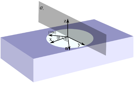
where and are the momentum operators, is the effective mass ( for GaAs, is the electron mass), while is the gating potential used to localize the electron in a QD. In the lateral system, symmetries that can be present are the -fold rotational symmetry and the vertical mirror plane symmetry . For simplicity, we assume that coincides with the plane of the QD coordinate frame (see FIG. 1). Thus, we assume a general form of the orbital Hamiltonian that has a or ( also) symmetry. Due to the symmetry, eigenenergies and eigenvectors of can be classified according to the irreducible representations (IRs) of a given point-group symmetry.
Besides , in Eq. (1) the Zeeman term appears, describing the coupling of spin and magnetic field:
| (2) |
where is the effective Landé factor ( for GaAs), is the Bohr magneton, is the electron’s spin, and is the in-plane magnetic field forming an angle with the crystallographic [100] axis. In Eq. (1) we have neglected the orbital effects of the in-plane magnetic field. This is a reasonable assumption for the magnetic field strength weaker than a few RSF11 . In the case of the magnetic field applied in the direction, orbital effects would be much more pronounced RSF11 .
Eigenstates of can be written in a direct product form , where corresponds to the eigenvectors of the Hamiltonian with an energy , while represents eigenvectors of with spin projection parallel or antiparallel to the magnetic field direction and an eigenenergy , respectively. The effect of on the eigenspectra of can be seen as the splitting of eigenenergies into two branches with an energy difference . In this work, we assume that is much weaker than the energy difference between the ground and the first excited state of the orbital Hamiltonian .
Besides () that acts trivially in the spin (orbital) space, the SOI Hamiltonian does not commute with . It consists of two terms, Dresselhaus DR and Rashba RA : the Dresselhaus term exists due to the bulk inversion asymmetry of the structure, while the Rashba term is present when an electric field perpendicular to the growth direction is applied. The form of spin-orbit coupling is dependent on the structure’s symmetry. For GaAs, having the zincblende structure, the SOI Hamiltonian is equal to
| (3) |
where and are Rashba and Dresselhaus coupling constants, while and are momentum operators in the [100] and [010] crystallographic directions, respectively. The electron spin is locked to the crystal momentum, since the potential trap confines electron of the crystal. Thus, an electron in a QD inherits the features of the crystal for which the crystal momentum is only appropriately defined. However, we have the choice to define the axis of our coordinate frame independently on the crystallographic [100] direction. Assuming that the angle between them is , and should be written in terms of momentum operators in the chosen frame: , .
The spin-orbit Hamiltonian can be written in a different form using the Rashba and Dresselhaus precession lengths,
| (4) |
To compare the ratio of the spin-orbit precession length and the orbital confinement length , we redefine and in terms of the overall spin-orbit length and the spin-orbit angle :
| (5) |
Since we assume no doping of the GaAs material SL05 , can be considered constant. Moreover, the relation RSF11 ; RPS+14 is satisfied in GaAs QDs, meaning that SOI can be treated as a perturbation.
Without SOI, qubit states can be defined as , where corresponds to the ground state of the spin-independent Hamiltonian . Because SOI can be treated on the level of a perturbation, we calculate first-order corrections of the qubit states due to spin-orbit coupling. Since it is known that the standard perturbation technique badly incorporates the spin-orbit-induced corrections CWL04 ; BSF10 , we follow the procedure explained in Ref. MSL16 : the Hamiltonian is transformed using the unitary operator , defined with the help of the position-dependent spin-orbit vector :
| (6) |
The unitary operator does not change the orbital and Zeeman Hamiltonian. On the other hand, the SOI Hamiltonian is transformed into
| (7) |
where is the orbital angular momentum. Using , the first-order correction of the qubit states can be written as
| (8) |
where the sum over corresponds to all orbital eigenvectors different from the ground state , while .
The lateral QD model is valid if the electron dynamics in the direction is suppressed; i.e., an electron is always in the ground state. Thus, we assume that confinement length in the direction is much stronger than in the plane. The Hamiltonian describing the quantum confinement in the direction is equal to , where for and for . To this Hamiltonian corresponds the following ground state (for ) SS03
| (9) |
where is the Airy function, while is the inverse of the characteristic length in the direction.
In order to simplify the notation, in the rest of the paper we assume that and represent SOI corrected qubit states in the -plane, while and correspond to wavefunctions of the qubit states in three dimensions.
III Rabi frequency and phonon induced spin relaxation rate
Electrical control of the spin qubit is possible by applying the in-plane oscillating electric field , resulting in the Rabi Hamiltonian . The Rabi frequency, measuring the speed of the single-qubit rotations, is equal to , where
| (10) |
is the dipole moment (in units), present due to the SOI induced spin mixing mechanism. Misalignment of the applied field direction and the dipole moment leads to a trivial suppression of the Rabi frequency. Since it is beneficial to increase the Rabi frequency as much as possible, the electric field should be applied in the direction of the dipole moment. Thus, for fixed , the maximal value of the Rabi frequency
| (11) |
is completely dependent on the strength of the dipole moment.
Since spin-phonon interaction in semiconductor QDs is irrelevant KN00 , unlike donor-bound electrons in direct band-gap semiconductors LKD+16 , only electron-phonon-induced transition between the qubit states should be considered in the study of spin relaxation. Electron-phonon coupling is triggered by the SOI-induced admixture mechanism, being highly dependent on the symmetry of the gating potential LKD+16 . We determine the rate of spin relaxation at from the Fermi golden rule,
| (12) |
assuming the dominant contribution of acoustic phonons, having an energy , equal to the level separation between the qubit states, . For magnetic field strengths up to a few T, relevant for this work, the linear dependence of phonon frequencies on the crystal wave vector length can be used, , giving us coorframe .
The geometric factor is dependent on the phonon mode, longitudinal (LA) or transverse (TA). The longitudinal geometric factor CBG+06
| (13) |
depends on both and , representing the deformation and piezoelectric constant, respectively. On the other hand, the transverse geometric factor CBG+06
is dependent on the piezoelectric constant solely. Other parameters for the GaAs material are CWL04 ; MSL16 , , , , , and .
Finally, in Eq. (12) both the lateral and the -direction confinement enter the relaxation rate through the scattering matrix element . We employ the dipole approximation , justified for magnetic field strengths below a few T.
To summarize, the phonon-induced relaxation rate can be divided into three separate channels: the deformation phonons , the longitudinal piezoelectric phonons , and the transverse piezoelectric phonons . In GaAs QDs, is the dominant relaxation channel, being two orders of magnitude stronger than in the dipole approximation regime. Thus, we can identify the total relaxation rate with CSZ+18 :
| (15) |
where . We assume a typical confinement length nm RSF11 ; RPS+14 of the GaAs QD in an experimental setup and magnetic field up to a few T (see Section II). Since confinement in the direction is much stronger than in the plane, , we conclude that is much weaker than 1. In other words, the influence of the confinement in the direction can be neglected.
Note that is squarely dependent on the absolute value of the dipole moment, meaning that the knowledge of the dipole moment is sufficient to fully explain the behavior of both the Rabi frequency and the spin relaxation rate.
IV Analytical expression for the dipole moment
Based on the previous conclusion, we come to the main objective: to derive symmetry allowed expression for the dipole moment. The results can be divided into three cases, according to the system’s group symmetry: (1) () and , (2) and , and (3) and .
IV.1 Dipole moment for systems with () or symmetry
To find the SOI-induced perturbative correction of the qubit states, we first rewrite the unitarily transformed SOI Hamiltonian in the coordinate frame of the potential,
| (16) | |||||
and neglect the second term in Eq. (7), assuming magnetic field strengths T needed to appropriately define the qubit states. For simplicity, we define two factors,
| (17) | |||||
| (18) |
with whose help can be written in a more compact form.
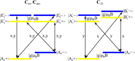
The Hamiltonian is in the orbital space dependent on the coordinates and that transform according to the IR . Their symmetry behavior restricts the states that can appear in the perturbative correction of the qubit states. It is simple to check that only states transforming according to the IR are allowed. This is illustrated in the left-hand panel of FIG. 2.
We label the ground state of the orbital Hamiltonian as , since the ground state in quantum mechanical systems is of the maximal possible symmetry LCC08 and it should transform according to the IR, representing the objects invariant under all group symmetry operations (see Table 1). We write two complex conjugate basis vectors of the two-dimensional IR as and , where labels the energy level. Also, we define the energy difference between the excited level and the ground state as .
| IR | ||||
| 0 | ||||
| -1 | ||||
| IR | ||||
| 0 | ||||
Due to the negative factor, the lowest qubit state is parallel to the magnetic field direction, while is the qubit state with spin projection antiparallel to the magnetic field direction. The first-order perturbative correction to the qubit states is written as . Thus, we can write the SOI corrected qubit states as , where the normalization factor is omitted as the correction is small. Correspondingly, the dipole moment is equal to
| (19) | |||||
Since , we approximate the unitary operator with , where is the identity matrix. After noticing that , , we find the SOI-induced corrections of the qubit states
| (20) | |||||
Additionally, transition dipole matrix elements are labeled as
| (21) |
Since the Zeeman splitting is much smaller than the orbital excitation energies, , the approximation can be made. Thus, Eq. (20) is transformed into
| (22) |
where and are the complex conjugates of and , respectively. Components of the dipole moment can now be written in a more compact form
| (23) |
where stands for the real part of . Potential dependent parameters that enter Eq. (23) are the transition dipole matrix elements and the excitation energies. Besides them, dipole moment components are dependent on the spin-orbit angle , magnetic field angle , and the angle between the [100] crystallographic direction and the axis.
A further simplification of Eq. (23) stems from the existence of the vertical mirror symmetry , requiring that must be zero. This can be proven in a few simple steps. First, we deduce from the matrix of an IR , representing the vertical mirror plane, that transforms one IR vector into the other, . Furthermore, remains unchanged, while acquires a minus sign, leading to the following behavior of the transition matrix elements and under vertical mirror plane symmetry:
| (24) |
From the previous relations, we conclude that the term transforms into , meaning that this object does not obey the symmetry of a system and must vanish.
Additionally, rotational symmetry of a system imposes that matrix elements and are equal. This can be concluded from the action of the rotation for an angle around the axis, being the element of the group symmetry. An element leaves the vector unchanged and adds a phase to the vector . Also, it transforms and to and . Thus, and are transformed into and , respectively. Correspondingly,
| (25) |
where we have neglected the term, which was previously proven to equal to zero. Since and must remain unchanged under the group symmetry operations, we conclude that the relation must hold. Thus, we have obtained a general relation for the dipole moment in the case of the potential symmetry ():
| (26) |
In these situations, the absolute value of the dipole moment is independent of the orientation of the potential with respect to the crystallographic frame.
Analogous analysis can be conducted in the case. Since the matrix form of the IRs and (see Table 1) for this symmetry group is the same as for , the procedure is exactly the same if the change in the previous discussion is made.
As an example, we implement the derived formula (26) in the case of the isotropic two-dimensional harmonic confinement with symmetry, assuming only one excited level in the perturbative correction of the qubit states. With the help of the states and , corresponding to the ground and the first excited states of the one-dimensional harmonic oscillator, we can define the ground state and two complex conjugate eigenstates and of the degenerate level: , , and . In this case, the squared norm of the transition matrix element is equal to . Using the energy difference of the ground and the first excited energy level and the confinement length , an expression for the dipole moment is obtained MSL16 :
| (27) |
IV.2 Dipole moment for systems with or symmetry
As the next step, we discuss potentials with symmetry. In this case, coordinates and transform according to the IRs and , respectively. Their symmetry behavior imposes the following: couples the ground state with states transforming according to the IR (see the right-hand panel of FIG. 2). Thus, the SOI-induced corrections of the qubit states are
| (28) | |||||
where is the energy difference between the energy level transforming according to the IR and the ground-state energy. We define the transition matrix elements as
| (29) |
and obtain the formula for the dipole moment,
| (30) |
In this case, anisotropy of the dipole moment appears since it is not forbidden that differs from .
The anisotropy of the dipole moment can be illuminated using the example of the anisotropic two-dimensional harmonic potential , with different confinement lengths and along the and directions. We set and , where is the measure of anisotropy. We assume two excited orbital states in the perturbative correction: one of type and one of type . In this case we define the ground state and two excited orbital states and , where represents the ground or first excited state (subscript 0 or 1, respectively) of the one-dimensional harmonic oscillator problem in the or direction. The obtained result
| (31) |
is again consistent with Ref. MSL16 .
In the case of the symmetry, using a similar analysis as in the previous case, we obtain the expression for the dipole moment
| (32) |
where , , and is the energy difference between the nondegenerate energy level transforming according to the IR and the ground-state energy.
IV.3 Dipole moment for systems with or symmetry
In the case of symmetry, all IRs () are one dimensional and represent an element of symmetry as . Besides the geometric symmetry, the time-reversal symmetry should be included also TIMrev . Time-reversal changes the sign of the quantum number labeling the IR vector , since it acts as a complex conjugation in the orbital space:
| (33) |
The eigenproblem of the Hamiltonian , when combined with the commutation relation , gives us
| (34) |
stating that, for , vectors and are eigenstates of the degenerate level . To this degenerate level corresponds the reducible representation (except for ). The representation is equivalent to the IR of the group (see Table 1) if the generator is neglected. In other words, Eq. (23) for the dipole moment is valid also in this case, since it is obtained without assuming the presence of vertical mirror symmetry. In this case vectors and coincide with and , respectively.
A further simplification of Eq. (23) appears for systems whose symmetry element is rotation. This happens if the relation () is satisfied. Since and in this case, Eq. (26) is relevant. Using the same reasoning it can be concluded that Eq. (26) is valid in the case also.
Finally, the dipole moment components for the symmetry are equal to
| (35) |
where , , and is the energy difference between the level transforming according to the IR and the ground-state energy.
To conclude, anisotropy of the potential orientation with respect to the crystallographic frame is present in systems without the group element (, ); isotropic behavior is present if a rotation for is the group element, i.e., if ( or .
V Applications: infinite-wall equilateral triangle, square, and rectangular potential
The results presented in the previous Section fully explain the dependence of the Rabi frequency and spin relaxation rate on the spin-orbit angle, magnetic field direction, and the relative orientation of the gating potential with respect to the crystallographic frame.
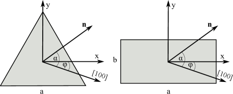
However, symmetry arguments alone cannot provide us with a qualitative estimation of the spin relaxation rate, corresponding to the phonon-allowed spin qubit lifetime. Since is known for the harmonic gating MSL16 , we wish to compare the phonon-induced spin relaxation rate of other confinement potentials with the known values. To this end, we analyze the spin qubit confined inside the infinite-wall equilateral triangle, square, and rectangular gating potential (see FIG. 3):
| (38) | |||||
| (41) |
In the first case, Eq. (38), the potential has symmetry and the corresponding eigenvectors of the spin-independent Hamiltonian transform according to the one-dimensional IRs and and two-dimensional IR of the group. The set of eigenenergies and eigenvectors , , and LB85 are dependent on two parameters and that have different sets of allowed values for each IR. Their concrete form is given in Appendix A.
In the second case, Eq. (41), the symmetry of the potential is dependent on the ratio : if , the symmetry of the problem is ; otherwise, is the symmetry of the spin-independent Hamiltonian . In both situations, eigenenergies and eigenvalues can be found by using the separation of variables. The set of eigenenergies and eigenvectors in this case is
| (42) | |||||
| (43) |
defined using the two independent parameters and that take integer values. However, these solutions do not have any definite symmetry CCM+05 . Therefore, they need to be symmetrized to apply the general results from Section IV. Symmetry-adapted eigenfunctions can be found in Appendix B.
After calculating the transition dipole matrix element and the excitation energies for two excited states in the perturbative correction check , we obtain the desired results
| (44) | |||||
| (45) |
where the first result corresponds to the infinite-wall equilateral triangle potential, while the second one is valid for both the infinite-wall square, , and rectangular, , potentials. Dipole moment constants and from Eqs. (44) and (45) suggest a much weaker dipole moment when compared to the harmonic gating of the same confinement length [see Eqs. (27) and (31)].
Using the relation , we conclude that square and rectangular confined QDs have a relaxation rate that is four orders of magnitude weaker than the harmonic potential; in the equilateral triangle case, a decrease of almost six orders of magnitude is observed. Thus, our result indicates a significant influence of the gating potential on the spin qubit lifetime and a beneficial role of the equilateral triangle confinement.
VI Conclusions
We have investigated the influence of the gating potential symmetry on the Rabi frequency and phonon-induced spin relaxation rate in a single-electron GaAs quantum dot. Our results suggest that, independently of the symmetry of the gating potential, both the Rabi frequency and spin relaxation rate are dependent on the orientation of the magnetic field and the spin-orbit angle. Additionally, in systems with , , and () symmetry, orientation of the quantum dot potential with respect to the crystallographic reference frame is another degree of freedom that can be used to tune the desired properties of the system. The validity of the approach is confirmed on the known results for the isotropic and anisotropic harmonic potential. Additionally, we have compared the spin qubit lifetime in the case of an infinite-wall rectangular, square and equilateral triangle gating with the harmonic confinement. Our results indicate the enhanced lifetime of the spin qubit, reaching an almost six-orders-of-magnitude increase in the case of the equilateral triangle gating. In the end, we emphasize that in the regime of strong electric field, nonlinear effects KGS12 ; RGP15 ; VP18 cannot be fully explained by the symmetry of the gating potential, thus placing the conclusions of our work in the weak driving regime solely.
Acknowledgements.
We thank Nenad Vukmirović for fruitful discussion. This research is funded by the Serbian Ministry of Science (Project ON171035) and the National Scholarship Programme of the Slovak Republic (ID 28226).Appendix A Particle in the infinite-wall equilateral triangle potential: eigenenergies and eigenvectors
Here we summarize the results from Ref. LB85 regarding the Schrödinger equation solution of the particle in the infinite-wall equilateral triangle potential, having symmetry. Due to the symmetry, eigenvectors transform according to the one-dimensional IRs and and the two-dimensional IR . The concrete forms of eigenenergies and eigenstates,
| (46) |
| (47) |
| (48) |
| (49) |
are dependent on two parameters and that have different allowed values for each IR.
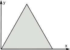
Note that the coordinate frame used to derive the previous equations (see FIG. 4) differs from the frame used in our work (see the left-hand panel of FIG. 3). To adapt the eigenfunction from Eqs. (47)-(49) to our case, a suitable change of coordinates and should be made.
Appendix B Particle in the infinite-wall square and rectangular potential: eigenvectors
The infinite-wall square potential has symmetry with the corresponding IRs , , and . Eigenvectors that transform according to the given IRs and the set of allowed quantum numbers are
| (50) |
| (51) |
| (52) |
| (53) |
| (54) |
In the case of the infinite-wall rectangular potential symmetry is relevant. Eigenfunctions transforming according to the IRs and and the corresponding set of quantum numbers are
| (55) |
| (56) |
| (57) |
| (58) |
In both cases, eigenenergies are given in Eq. (42) ( in the case and for the symmetry).
References
- (1) M. A. Nielsen and I. L. Chuang, Quantum Computation and Quantum Information, Cambridge University Press, (2010).
- (2) C. H. Bennett and D. P. DiVincenzo, Nature 404, 247-255 (2000).
- (3) D. Loss and D. P. DiVincenzo, Phys. Rev. A 57, 120 (1998).
- (4) T. P. Orlando, J. E. Mooij, L. Tian, C. H. van der Wal, L. S. Levitov, S. Lloyd, and J. J. Mazo, Phys. Rev. B 60, 15398 (1999).
- (5) Y. Nakamura, Yu. A. Pashkin, and J. S. Tsai, Nature 398, 786-788 (1999).
- (6) M. Yamamoto, S. Takada, C. Bäuerle, K. Watanabe, A. D. Wieck, and S. Tarucha, Nat. Nanotechnol. 7, 247-251 (2012).
- (7) E. I. Rashba, Sov. Phys. Solid State 2, 1109 (1960).
- (8) V. N. Golovach, M. Borhani, and D. Loss, Phys. Rev. B 74, 165319 (2006).
- (9) D. V. Bulaev and D. Loss, Phys. Rev. Lett. 98, 097202 (2007).
- (10) K. C. Nowack, F. H. L. Koppens, Yu. V. Nazarov, and L. M. K. Vandersypen, Science 318, 1430-1433 (2007).
- (11) E. I. Rashba, Phys. Rev. B 78, 195302 (2008).
- (12) R. Brunner, Y.-S. Shin, T. Obata, M. Pioro-Ladrière, T. Kubo, K. Yoshida, T. Taniyama, Y. Tokura, and S. Tarucha, Phys. Rev. Lett. 107, 146801 (2011).
- (13) E. Kawakami, P. Scarlino, D. R. Ward, F. R. Braakman, D. E. Savage, M. G. Lagally, Mark Friesen, S. N. Coppersmith, M. A. Eriksson, and L. M. K. Vandersypen, Nat. Nanotechnol. 9, 666-670 (2014).
- (14) K. Takeda, J. Yoneda, T. Otsuka, T. Nakajima, M. R. Delbecq, G. Allison, Y. Hoshi, N. Usami, K. M. Itoh, S. Oda, T. Kodera, and S. Tarucha, npj Quantum Inf. 4, 54 (2018).
- (15) D. V. Khomitsky, E. A. Lavrukhina, and E. Ya. Sherman, Phys. Rev. B 99, 014308 (2019).
- (16) S. Studenikin, M. Korkusinski, M. Takahashi, J. Ducatel, A. Padawer-Blatt, A. Bogan, D. Guy Austing, L. Gaudreau, P. Zawadzki, A. Sachrajda, Y. Hirayama, L. Tracy, J. Reno, and T. Hargett, Commun. Phys. 2, 159 (2019).
- (17) A. V. Khaetskii and Y. V. Nazarov, Phys. Rev. B 61, 12639 (2000); A. V. Khaetskii and Y. V. Nazarov, Phys. Rev. B 64, 125316 (2001).
- (18) P. Stano and J. Fabian, Phys. Rev. B 72, 155410 (2005).
- (19) V. N. Stavrou, J. Phys.: Condens. Matter 29, 485301 (2017); V. N. Stavrou, J. Phys.: Condens. Matter 30, 455301 (2018).
- (20) Z.-H. Liu, R. Li, X. Hu and J. Q. You, Sci. Rep. 8, 2302 (2018).
- (21) J. I. Climente, A. Bertoni, G. Goldoni, M. Rontani, and E. Molinari, Phys. Rev. B 75, 081303(R) (2007).
- (22) O. Malkoc, P. Stano, and D. Loss, Phys. Rev. B 93, 235413 (2016).
- (23) D. Chaney and P. A. Maksym, Phys. Rev. B 75, 035323 (2007).
- (24) V. I. Fal’ko, B. L. Altshuler, and O. Tsyplyatyev, Phys. Rev. Lett. 95, 076603 (2005).
- (25) P. Scarlino, E. Kawakami, P. Stano, M. Shafiei, C. Reichl, W. Wegscheider, and L. M. K. Vandersypen, Phys. Rev. Lett. 113, 256802 (2014).
- (26) O. Olendski and T. V. Shahbazyan, Phys. Rev. B 75, 041306(R) (2007).
- (27) S. Amasha, K. MacLean, I. P. Radu, D. M. Zumbühl, M. A. Kastner, M. P. Hanson, and A. C. Gossard, Phys. Rev. Lett. 100, 046803 (2008).
- (28) J. Planelles, F. Rajadell, and J. I. Climente, Phys. Rev. B 92, 041302(R) (2015).
- (29) M. Raith, P. Stano, and J. Fabian, Phys. Rev. B 83, 195318 (2011).
- (30) G. Dresselhaus, Phys. Rev. 100, 580 (1955).
- (31) E. I. Rashba, Fiz. Tv. Tela (Leningrad) 2, 1224 (1960); Sov. Phys. Solid State 2, 1109 (1960).
- (32) E. Ya. Sherman and D. J. Lockwood, Phys. Rev. B 72, 125340 (2005).
- (33) M. Raith, T. Pangerl, P. Stano, and J. Fabian, Phys. Status Solidi b 251, 1924 (2014).
- (34) J. L. Cheng, M. W. Wu, and C. Lü, Phys. Rev. B 69, 115318 (2004).
- (35) F. Baruffa, P. Stano, and J. Fabian, Phys. Rev. Lett. 104, 126401 (2010).
- (36) R. de Sousa and S. Das Sarma, Phys. Rev. B 68, 155330 (2003).
- (37) X. Linpeng, T. Karin, M. V. Durnev, R. Barbour, M. M. Glazov, E. Ya. Sherman, S. P. Watkins, S. Seto, and K.-M. C. Fu, Phys. Rev. B 94, 125401 (2016).
- (38) Note that both the wave vector and the electron coordinate are written in the crystallographic reference frame.
- (39) J. I. Climente, A. Bertoni, G. Goldoni, and E. Molinari, Phys. Rev. B 74, 035313 (2006).
- (40) L. C. Camenzind, L. Yu, P. Stano, J. D. Zimmerman, A. C. Gossard, D. Loss, and D. M. Zumbühl, Nat. Commun. 9, 3454 (2018).
- (41) E. Lijnen, L. F. Chibotaru, and A. Ceulemans, Phys. Rev. E 77, 016702 (2008).
- (42) L. Jansen and M. Boon, Theory of Finite Groups: Applications in Physics, North Holland, Amsterdam, (1967); M. Damnjanović, O simetriji u kvantnoj nerelativističkoj fizici, Fizički fakultet, Beograd (2000). http://www.ff.ac.rs/Katedre/QMF/SiteQMF/pdf/sknf2e.pdf
- (43) In the case of groups, time-reversal is the symmetry of the system. However, it can be checked that can be safely neglected. Time-reversal in the case of vectors from one-dimensional IRs has a trivial action. In the case of the two-dimensional IRs time-reversal transforms one vector of the IR into the other; in other words, it has the same behavior as the vertical mirror plane symmetry and can be ignored.
- (44) W.-K. Li and S. M. Blinder, J. Math. Phys. 26, 2784 (1985).
- (45) L. F. Chibotaru, A. Ceulemans, M. Morelle, G. Teniers, C. Carballeira, and V. V. Moshchalkov, J. Math. Phys. 46, 095108 (2005).
- (46) We have explicitly checked that other states appearing in the perturbative expansion can be safely ignored.
- (47) D. V. Khomitsky, L. V. Gulyaev, and E. Ya. Sherman, Phys. Rev. B 85, 125312 (2012).
- (48) J. Romhányi, G. Burkard, and A. Pályi, Phys. Rev. B 92, 054422 (2015).
- (49) M. T. Veszeli and A. Pályi, Phys. Rev. B 97, 235433 (2018).