Control-Aware Representations for Model-based Reinforcement Learning
Abstract
A major challenge in modern reinforcement learning (RL) is efficient control of dynamical systems from high-dimensional sensory observations. Learning controllable embedding (LCE) is a promising approach that addresses this challenge by embedding the observations into a lower-dimensional latent space, estimating the latent dynamics, and utilizing it to perform control in the latent space. Two important questions in this area are how to learn a representation that is amenable to the control problem at hand, and how to achieve an end-to-end framework for representation learning and control. In this paper, we take a few steps towards addressing these questions. We first formulate a LCE model to learn representations that are suitable to be used by a policy iteration style algorithm in the latent space. We call this model control-aware representation learning (CARL). We derive a loss function for CARL that has close connection to the prediction, consistency, and curvature (PCC) principle for representation learning. We derive three implementations of CARL. In the offline implementation, we replace the locally-linear control algorithm (e.g., iLQR) used by the existing LCE methods with a RL algorithm, namely model-based soft actor-critic, and show that it results in significant improvement. In online CARL, we interleave representation learning and control, and demonstrate further gain in performance. Finally, we propose value-guided CARL, a variation in which we optimize a weighted version of the CARL loss function, where the weights depend on the TD-error of the current policy. We evaluate the proposed algorithms by extensive experiments on benchmark tasks and compare them with several LCE baselines.
1 Introduction
Control of non-linear dynamical systems is a key problem in control theory. Many methods have been developed with different levels of success in different classes of such problems. The majority of these methods assume that a model of the system is known and the underlying state of the system is low-dimensional and observable. These requirements limit the usage of these techniques in controlling dynamical systems from high-dimensional raw sensory data (e.g., image and audio), where the system dynamics is unknown, a scenario often seen in modern reinforcement learning (RL).
Recent years have witnessed the rapid development of a large arsenal of model-free RL algorithms, such as DQN (Mnih et al., 2013), TRPO (Schulman et al., 2015a), PPO (Schulman et al., 2017), and SAC (Haarnoja et al., 2018), with impressive success in solving high-dimensional control problems. However, most of this success has been limited to simulated environments (e.g., computer games), mainly due to the fact that these algorithms often require a large number of samples from the environment. This restricts their applicability in real-world physical systems, for which data collection is often a difficult process. On the other hand, model-based RL algorithms, such as PILCO (Deisenroth and Rasmussen, 2011), MBPO (Janner et al., 2019), and Visual Foresight (Ebert et al., 2018), despite their success, still have many issues in handling the difficulties of learning a model (dynamics) in a high-dimensional (pixel) space.
To address this issue, a class of algorithms have been developed that are based on learning a low-dimensional latent (embedding) space and a latent model (dynamics), and then using this model to control the system in the latent space. This class has been referred to as learning controllable embedding (LCE) and includes recently developed algorithms, such as E2C (Watter et al., 2015), RCE (Banijamali et al., 2018), SOLAR (Zhang et al., 2019), PCC (Levine et al., 2020), Dreamer (Hafner et al., 2020), and PC3 (Shu et al., 2020). The following two properties are extremely important in designing LCE models and algorithms. First, to learn a representation that is the most suitable for the control process at hand. This suggests incorporating the control algorithm in the process of learning representation. This view of learning control-aware representations is aligned with the value-aware and policy-aware model learning, VAML (Farahmand, 2018) and PAML (Abachi et al., 2020), frameworks that have been recently proposed in model-based RL. Second, to interleave the representation learning and control processes, and to update them both, using a unifying objective function. This allows to have an end-to-end framework for representation learning and control.
LCE methods, such as SOLAR and Dreamer, have taken steps towards the second objective by performing representation learning and control in an online fashion. This is in contrast to offline methods like E2C, RCE, PCC, and PC3, that learn a representation once and then use it in the entire control process. On the other hand, methods like PCC and PC3 address the first objective by adding a term to their representation learning loss function that accounts for the curvature of the latent dynamics. This term regularizes the representation towards smoother latent dynamics, which are suitable for the locally-linear controllers, e.g., iLQR (Li and Todorov, 2004), used by these methods.
In this paper, we take a few steps towards the above two objectives. We first formulate a LCE model to learn representations that are suitable to be used by a policy iteration (PI) style algorithm in the latent space. We call this model control-aware representation learning (CARL). We derive a loss function for CARL that exhibits a close connection to the prediction, consistency, and curvature (PCC) principle for representation learning, proposed in Levine et al. (2020). We derive three implementations of CARL: offline, online, and value-guided. Similar to offline LCE methods, such as E2C, RCE, PCC, and PC3, in offline CARL, we first learn a representation and then use it in the entire control process. However, in offline CARL, we replace the locally-linear control algorithm (e.g., iLQR) used by these LCE methods with a PI-style (actor-critic) RL algorithm. Our choice of RL algorithm is the model-based implementation of soft actor-critic (SAC) (Haarnoja et al., 2018). Our experiments show significant performance improvement by replacing iLQR with SAC. Online CARL is an iterative algorithm in which at each iteration, we first learn a latent representation by minimizing the CARL loss, and then perform several policy updates using SAC in this latent space. Our experiments with online CARL show further performance gain over its offline version. Finally, in value-guided CARL (V-CARL), we optimize a weighted version of the CARL loss function, in which the weights depend on the TD-error of the current policy. This would help to further incorporate the control algorithm in the representation learning process. We evaluate the proposed algorithms by extensive experiments on benchmark tasks and compare them with several LCE baselines.
2 Problem Formulation
We are interested in learning control policies for non-linear dynamical systems, where the states are not fully observed and we only have access to their high-dimensional observations . This scenario captures many practical applications in which we interact with a system only through high-dimensional sensory signals, such as image and audio. We assume that the observations have been selected such that we can model the system in the observation space using a Markov decision process (MDP)111A method to ensure observations are Markovian is to buffer them for several time steps (Mnih et al., 2013). , where and are observation and action spaces; is the reward function with maximum value , defined by the designer of the system to achieve the control objective;222For example, in a goal tracking problem in which the agent (robot) aims at finding the shortest path to reach the observation goal (the observation corresponding to the goal state ), we may define the reward for each observation as the negative of its distance to , i.e., . is the unknown transition kernel; and is the discount factor. Our goal is to find a mapping from observations to control signals, , with maximum expected return, i.e., .
Since the observations are high-dimensional and the observation dynamics is unknown, solving the control problem in the observation space may not be efficient. As discussed in Section 1, the class of learning controllable embedding (LCE) algorithms addresses this issue by learning a low-dimensional latent (embedding) space and a latent state dynamics, and controlling the system there. The main idea behind LCE is to learn an encoder , a latent space dynamics , and a decoder ,333Some recent LCE models, such as PC3 (Shu et al., 2020), are advocating latent models without a decoder. Although we are aware of the merits of such approach, we use a decoder in the models proposed in this paper. such that a good or optimal controller (policy) in minimizes the expected loss in the observation space . This means that if we model the control problem in as a MDP and solve it using a model-based RL algorithm to obtain a policy , the image of in the observation space, i.e., , should have a high return. Thus, the loss function to learn and from observations should be designed to comply with this goal.
This is why in this paper, we propose a LCE framework that tries to incorporate the control algorithm used in the latent space in the representation learning process. We call this model, control-aware representation learning (CARL). In CARL, we set the class of control (RL) algorithms used in the latent space to approximate policy iteration (PI), and more specifically to soft actor-critic (SAC) (Haarnoja et al., 2018). Before describing CARL in details in the following sections, we present a number of useful definitions and notations here.
For any policy in , we define its value function and Bellman operator as
| (1) |
for all and , where and are the reward function and dynamics induced by .
Similarly, for any policy in , we define its induced reward function and dynamics as and . We also define its value function and Bellman operator , for all and , as
| (2) |
For any policy and value function in the latent space , we denote by and , their image in the observation space , given encoder , and define them as
| (3) |
3 A Control Perspective for CARL Model
In this section, we formulate our LCE model, which we refer to as control-aware representation learning (CARL). As described in Section 2, CARL is a model for learning a low-dimensional latent space and the latent dynamics, from data generated in the observation space , such that this representation is suitable to be used by a policy iteration (PI) algorithm in . In order to derive the loss function used by CARL to learn and its dynamics, i.e., , we first describe how the representation learning can be interleaved with PI in . Algorithm 1 contains the pseudo-code of the resulting algorithm, which we refer to as latent space learning policy iteration (LSLPI).
Each iteration of LSLPI starts with a policy in the observation space , which is the mapping of the improved policy in in iteration , i.e., , back in through the encoder (Lines 6 and 7). We then compute , the current policy in , as the image of in through the encoder (Line 4). Note that is the encoder learned at the end of iteration (Line 8). We then use the latent space dynamics learned at the end of iteration (Line 8), and first compute the value function of in the policy evaluation or critic step, i.e., (Line 5), and then use to compute the improved policy , as the greedy policy w.r.t. , i.e., , in the policy improvement or actor step (Line 6). Using the samples in the buffer , together with the current policies in , i.e., and , we learn the new representation (Line 8). Finally, we generate samples by following , the image of the improved policy back in using the old encoder (Line 7), and add it to the buffer (Line 9), and the algorithm iterates. It is important to note that both critic and actor operate in the low-dimensional latent space .
LSLPI is a PI algorithm in . However, what is desired is that it also acts as a PI algorithm in , i.e., it results in (monotonic) policy improvement in , i.e., . Therefore, we define the representation learning loss function in CARL, such that it ensures that LSLPI also results in policy improvement in . The following theorem, whose proof is reported in Appendix B, shows the relationship between the value functions of two consecutive polices generated by LSLPI in .
Theorem 1.
Let , , , , and be the policies , , , , and the learned latent representation at iteration of the LSLPI algorithm (Algorithm 1). Then, the following holds for the value functions of and :
| (4) |
for all , where the error term for a policy is given by
| (5) | ||||
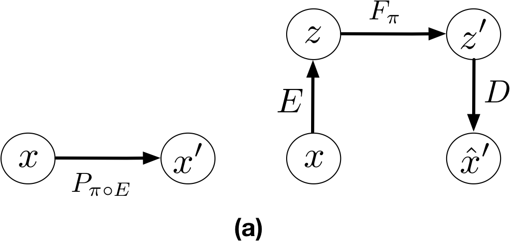
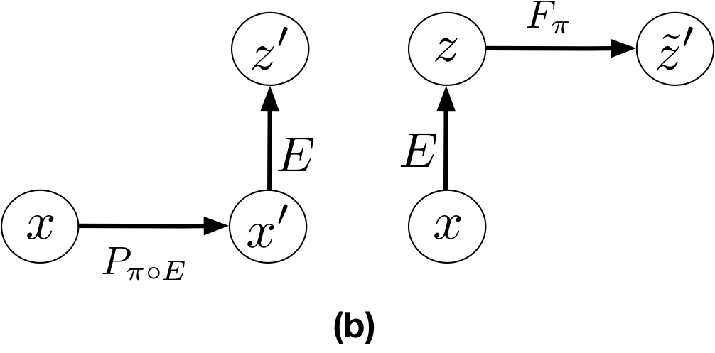
It is easy to see that LSLPI guarantees (policy) improvement in , if the terms in the parentheses on the RHS of (4) are zero. We now describe these terms. The last term on the RHS of (4) is the KL between and . This term can be seen as a regularizer to keep the new encoder close to the old one . The four terms in (5) are: (I) The encoding-decoding error to ensure ; (II) The error that measures the mismatch between the reward of taking action according to policy at , and the reward of taking action according to policy at the image of in under ; (III) The error in predicting the next observation through paths in and . This is the error between and shown in Fig. 1(a); and (IV) The error in predicting the next latent state through paths in and . This is the error between and shown in Fig. 1(b).
Representation Learning in CARL: Theorem 1 provides us with a recipe (loss function) to learn the latent space and . In CARL, we propose to learn a representation for which the terms in the parentheses on the RHS of (4) are small. As mentioned earlier, the second term, , can be considered as a regularizer to keep the new encoder close to the old one . Term (II) that measures the mismatch between rewards can be kept small, or even zero, if the designer of the system selects the rewards in a compatible way. Although CARL allows us to learn a reward function in the latent space, similar to several other LCE works (Watter et al., 2015; Banijamali et al., 2018; Levine et al., 2020; Shu et al., 2020), in this paper, we assume that a compatible reward function is given. Terms (III) and (IV) are the equivalent of the prediction and consistency terms in PCC (Levine et al., 2020) for a particular latent space policy . Since PCC has been designed for an offline setting (i.e., one-shot representation learning and control), the prediction and consistency terms are independent of a particular policy and are defined for state-action pairs. While CARL is designed for an online setting (i.e., interleaving representation learning and control), and thus, its loss function at each iteration depends on the current latent space policies and . As we will see in Section 4.1, our offline implementation of CARL uses a loss function very similar to that of PCC. Note that (IV) is slightly different than the consistency term in PCC. However, if we upper-bound it using Jensen inequality as , we obtain the loss term , which is very similar to the consistency term in PCC. Similar to PCC, we also add a curvature loss to the loss function of CARL to encourage having a smoother latent space dynamics . Putting all these terms together, we obtain the CARL loss function as
| (6) |
where are hyper-parameters of the algorithm, are the encoding-decoding and prediction losses defined in (5), is the consistency loss defined above, is the curvature loss, and is the regularizer that ensures the new encoder remains close to the old one. We set to a small value not to allow to play a major role in our implementations.
4 Different Implementations of CARL
The CARL loss function in (6) introduces an optimization problem that takes a policy as input and learns a representation suitable for its evaluation and improvement. To optimize this loss in practice, similar to the PCC model (Levine et al., 2020), we define as a latent variable model that factorizes as , and use a variational approximation to the interactable negative log-likelihood of the loss terms in (6). The variational bounds for these terms can be obtained similar to Eqs. 6 and 7 in Levine et al. (2020). Below we describe three instantiations of the CARL model in practice. Implementation details can be found in Algorithm 2 in Appendix E. While CARL is compatible with most PI-style (actor-critic) RL algorithms, following a recent work, MBRL (Janner et al., 2019), we choose SAC as the RL algorithm in CARL. Since most actor-critic algorithms are based on first-order gradient updates, as discussed in Section 3, we regularize the curvature of the latent dynamics (see Eqs. 8 and 9 in Levine et al. 2020) in CARL to improve its empirical stability and performance in policy learning.
4.1 Offline CARL
We first implement CARL in an offline setting, where we first generate a (relatively) large batch of observation samples using an exploratory (e.g., random) policy. We then use this batch to optimize the CARL loss function (6) via a variational approximation scheme, as described above, and learn a latent representation and . Finally, we solve the decision problem in using a model-based RL algorithm, which in our case is model-based soft actor-critic (SAC) (Haarnoja et al., 2018). The learned policy in is then used to control the system from observations as . This is the setting that has been used in several recent LCE works, such as E2C (Watter et al., 2015), RCE (Banijamali et al., 2018), PCC (Levine et al., 2020), and PC3 (Shu et al., 2020). Our offline implementation is different than these works in 1) we replace the locally linear control algorithm, namely iterative LQR (iLQR) (Li and Todorov, 2004), used in them with model-based SAC, which results in significant performance improvement as shown in our experimental results in Section 5, and 2) we optimize the CARL loss function that as mentioned above, despite close connection is still different than the one used by PCC.
The CARL loss function presented in Section 3 has been designed for an online setting in which at each iteration, it takes a policy as input and learns a representation that is suitable for evaluating and improving this policy. However, in the offline setting, the learned representation should be good for any policy generated in the course of running the PI-style control algorithm. Therefore, we marginalize out the policy from the (online) CARL’s loss function and use the RHS of the following corollary (proof in Appendix C) to construct the CARL loss function used in our offline experiments.
Corollary 2.
Let and be two consecutive policies in genrated by a PI-style control algorithm in the latent space constructed by . Then, the following holds for the value functions of and , where is defined by (5) (in modulo to replacing sampled action with action ):
| (7) |
4.2 Online CARL
In the online implementation of CARL, at each iteration , the current policy is the improved policy of the last iteration, . We first generate a relatively (to offline CARL) small batch samples from the image of this policy in , i.e., , and then learn a representation suitable for evaluating and improving the image of in under the new encoder . This means that with the new representation, the current policy that was the image of in under , should be replaced by its image under the new encoder, i.e., . In online CARL, this is done by a policy distillation step in which we minimize the following loss:444Our experiments reported in Appendix G show that adding distillation improves the performance in online CARL. Thus, all the results reported for online CARL and value-guided CARL in the main paper are with policy distillation.
| (8) |
After the current policy was set, we perform multiple steps of (model-based) SAC in using the current model, , and then send the resulting policy to the next iteration.
4.3 Value-Guided CARL
In the previous two implementations of CARL, we learn the model using the loss function (6). Theorem 1 shows that minimizing this loss guarantees performance improvement. While this loss depends on the current policy (through the latent space policy and encoder), it does not use its value function . To incorporate this extra piece of information in the representation learning process, we utilize results from variational model-based policy optimization (VMBPO) work by Chow et al. (2020). Using Lemma 3 in Chow et al. (2020), we can include the value function in the observation space dynamics as555In general, this can also be applied to reward learning, but for simplicity we only focus on learning dynamics.
| (9) |
where is the risk-adjusted value function of policy , and is its corresponding state-action value function, i.e., . The reason for referring to and as risk-adjusted value functions is that the Bellman operator is no longer defined by the expectation operator over , but instead is defined by the exponential risk , with the temperature parameter (Ruszczyński and Shapiro, 2006). The modified dynamics is a re-weighting of using the exponential-twisting weights , where is the temporal difference (TD) error of the risk-adjusted value functions.
To incorporate the value-guided transition model into the CARL loss function, we need to modify all the loss terms that depend on , i.e., the prediction loss and the consistency loss . Because of the regularization term that enforces the policy to be close to , we may replace the transition dynamics in the prediction loss with . Since does not depend on the representation, minimizing the prediction loss would be equivalent to maximizing the expected log-likelihood (MLE) . Now if we replace dynamics with its value-guided counterpart in the MLE loss, we obtain the modified prediction loss
| (10) |
which corresponds to a weighted MLE loss in which the weights are the exponential TD errors.
Using analogous arguments, we may write the value-guided version of the consistency loss as
| (11) |
To complete the value-guided CARL (V-CARL) implementation, we need to compute the risk-adjusted value functions and to construct the weight . Here we provide a recipe for the case when is small (see Appendix D for details), in which the risk-adjusted value functions can be approximated by their risk-neutral counterparts, i.e., , and . Following Lemma 7 in Appendix A, we can approximate with and with . Together with the compatibility of the rewards, i.e., , the weight can be approximated by , which is simply the TD error in the latent space.
5 Experimental Results
In this section, we experiment with the following continuous control domains (see Appendix F for more descriptions): (i) Planar System, (ii) Inverted Pendulum, (iii) Cartpole, (iv) 3-link manipulator, and compare the performance of our CARL algorithms with two LCE baselines: PCC (Levine et al., 2020) and SOLAR (Zhang et al., 2019). These tasks have underlying start and goal states that are “not” observable to the algorithms, instead the algorithms only have access to the start and goal image observations. To evaluate the performance of the control algorithms, similar to Levine et al. (2020), we report the -time spent in the goal. The initial policy that is used for data generation is uniformly random. To measure performance reproducibility for each experiment, we 1) train models and 2) perform control tasks for each model. For SOLAR, due to its high computation cost we only train and evaluate different models. Besides the average results, we also report the results from the best LCE models, averaged over the control tasks.
General Results
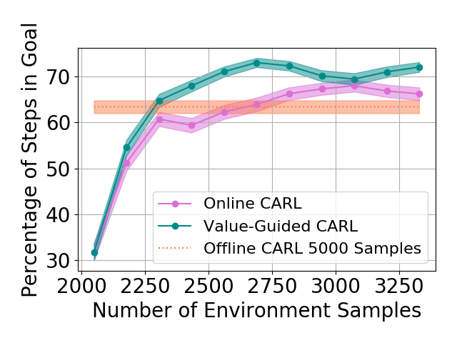
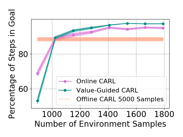
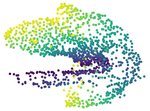
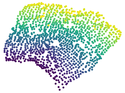
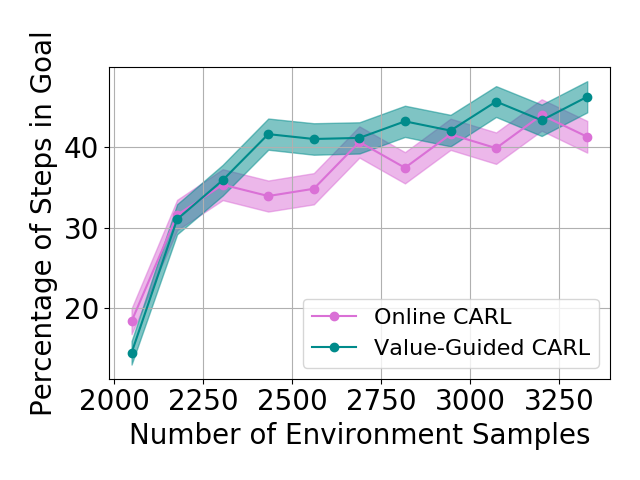
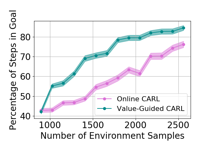
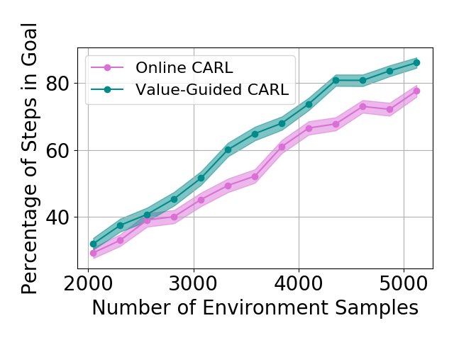
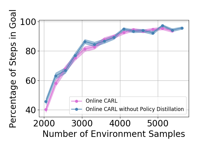
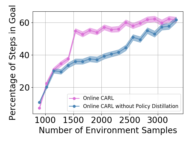
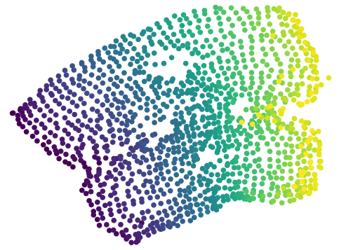
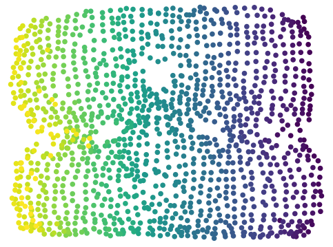
Table 1 shows the mean and standard deviations of the metrics on different control tasks. To compare the data efficiency of different methods, we also report the number of samples required to train the latent space and controller in each method. Our main experimental observation is four-fold. First, by replacing the iLQR control algorithm used by PCC with model-based SAC, offline CARL achieves significantly better performance in all of the tasks. This can be attributed to the advantage that SAC is more robust and effective operating in non-(locally)-linear environments. More details in the comparisons between PCC and offline CARL can be found in Appendix G, in which we explicitly compare their control performance and latent representation maps. Second, in all the tasks online CARL is more data-efficient than the offline counterparts, i.e., we can achieve similar or better performance with fewer environment samples. In particular, online CARL is notably superior in the planar, cartpole, and swingup tasks, in which similar performance can be achieved with , , and times less samples, respectively (see Figure 2). From Figure 3, interestingly the latent representations of online CARL also tend to improve progressively with the value of the policy. Third, in the simpler tasks (Planar, Swingup, Cartpole), value-guided CARL (V-CARL) manages to achieve even better performance. This corroborates with our hypothesis that extra improvement can be delivered by CARL when its LCE model is more accurate in regions of the space with higher temporal difference — regions with higher anticipated future return. Unfortunately, in three-pole, the performance of V-CARL is worse than its online counterpart. This is likely due to instability in representation learning when the sample variance is amplified by the exponential-TD weight. Finally, SOLAR requires much more samples to learn a reasonable latent space for control, and with limited data it fails to converge to a good policy. Note that we are able to obtain better results in the planar task when the goal location is fixed (see Appendix 3). Yet even with the fine-tuned latent space from Zhang et al. (2019), its performance is incomparable with that of CARL algorithms.
| Environment | Algorithm | Number of Samples | Avg -Goal | Best -Goal |
|---|---|---|---|---|
| Planar | PCC | 5000 | ||
| Planar | Offline CARL | 5000 | ||
| Planar | Online CARL | 3072 | ||
| Planar | Value-Guided CARL | 3200 | ||
| Planar | SOLAR | 5000 (VAE) + 16000 (Control) | ||
| Swingup | PCC | 5000 | ||
| Swingup | Offline CARL | 5000 | ||
| Swingup | Online CARL | 1408 | ||
| Swingup | Value-Guided CARL | 1408 | ||
| Swingup | SOLAR | 5200 (VAE) + 40000 (Control) | ||
| Cartpole | PCC | 10000 | ||
| Cartpole | Offline CARL | 10000 | ||
| Cartpole | Online CARL | 5120 | ||
| Cartpole | Value-Guided CARL | 5120 | ||
| Cartpole | SOLAR | 5000 (VAE) + 40000 (Control) | ||
| Three-pole | PCC | 4096 | ||
| Three-pole | Offline CARL | 4096 | ||
| Three-pole | Online CARL | 2944 | ||
| Three-pole | Value-Guided CARL | 2816 | ||
| Three-pole | SOLAR | 2000 (VAE) + 20000 (Control) |

Results with Environment-biased Sampling
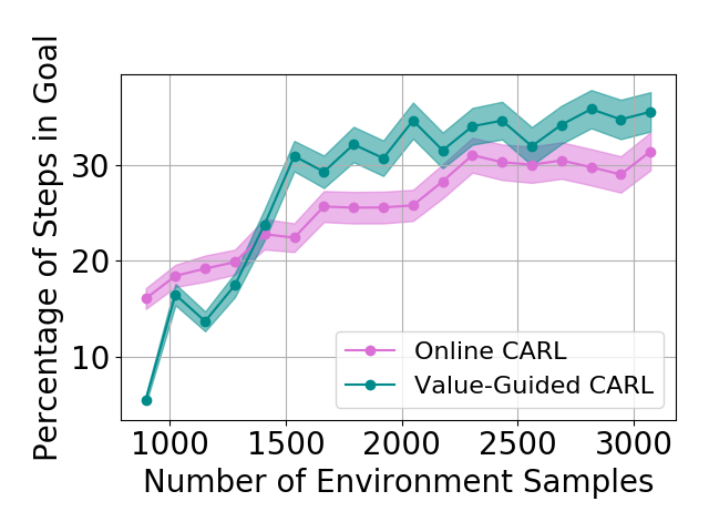
In the previous experiments, all the online LCE algorithms are warm-started with data collected by a uniformly random policy over the entire environment. With this uniform data collection, we do not observe a significant difference between online CARL and V-CARL. This is because with sufficient data the LCE dynamics is accurate enough on most parts of the state-action space for control. To further illustrate the advantage of V-CARL over online CARL, we modify the experimental setting by gathering initial samples only from a specific region of the environment (see Appendix F for details). Figure 4 shows the learning curves of online CARL and V-CARL in this case. Clearly with biased initial data both algorithms experience a certain level of performance degradation. Yet, V-CARL clearly outperforms online CARL. This again verifies our conjecture that value-aware LCE models are more robust to initial data distribution and more superior in policy optimization.
6 Conclusions
In this paper, we argued for incorporating control in the representation learning process and for the interaction between control and representation learning in learning controllable embedding (LCE) algorithms. We proposed a LCE model called control-aware representation learning (CARL) that learns representations suitable for policy iteration (PI) style control algorithms. We proposed three implementations of CARL that combine representation learning with model-based soft actor-critic (SAC), as the controller, in offline and online fashions. In the third implementation, called value-guided CARL, we further included the control process in representation learning by optimizing a weighted version of the CARL loss function, in which the weights depend on the TD-error of the current policy. We evaluated the proposed algorithms on benchmark tasks and compared them with several LCE baselines. The experiments show the importance of SAC as the controller and of the online implementation. Future directions include 1) investigating other PI-style algorithms in place of SAC, 2) developing LCE models suitable for value iteration style algorithms, and 3) identifying other forms of bias for learning an effective embedding and latent dynamics.
Broader Impact
Controlling non-linear dynamical systems from high-dimensional observation is challenging. Direct application of model-free and model-based reinforcement learning algorithms to this problem may not be efficient, due to requiring a large number of samples from the real system (model-free) and the challenges of learning a model in a high-dimensional space (model-based). A popular approach to address this problem is learning controllable embedding (LCE), i.e., learning a low-dimensional latent space and a latent space model, and performing the optimal control in this learned latent space. This work is a step towards end-to-end representation learning and control in this setting. We propose methods that interleave representation learning and control, which allows us to learn control-aware representations, i.e., representations that are suitable for the control problem at hand.
References
- Abachi et al. [2020] R. Abachi, M. Ghavamzadeh, and A. Farahmand. Policy-aware model learning for policy gradient methods. preprint arXiv:2003.00030, 2020.
- Banijamali et al. [2018] E. Banijamali, R. Shu, M. Ghavamzadeh, H. Bui, and A. Ghodsi. Robust locally-linear controllable embedding. In Proceedings of the Twenty First International Conference on Artificial Intelligence and Statistics, pages 1751–1759, 2018.
- Borkar [2002] V. Borkar. Q-learning for risk-sensitive control. Mathematics of operations research, 27(2):294–311, 2002.
- Breivik and Fossen [2005] M. Breivik and T. Fossen. Principles of guidance-based path following in 2D and 3D. In Proceedings of the 44th IEEE Conference on Decision and Control, pages 627–634, 2005.
- Chow et al. [2020] Y. Chow, B. Cui, M. Ryu, and M. Ghavamzadeh. Variational model-based policy optimization. In arXiv, 2020.
- Deisenroth and Rasmussen [2011] M. Deisenroth and C. Rasmussen. PILCO: A model-based and data-efficient approach to policy search. In Proceedings of the 28th International Conference on Machine Learning, page 465–472, 2011.
- Ebert et al. [2018] F. Ebert, C. Finn, S. Dasari, A. Xie, A. Lee, and S. Levine. Visual Foresight: Model-based deep reinforcement learning for vision-based robotic control. preprint arXiv:1812.00568, 2018.
- Farahmand [2018] A. Farahmand. Iterative value-aware model learning. In Advances in Neural Information Processing Systems 31, pages 9072–9083, 2018.
- Furuta et al. [1991] K. Furuta, M. Yamakita, and S. Kobayashi. Swing up control of inverted pendulum. In Proceedings of International Conference on Industrial Electronics, Control and Instrumentation, pages 2193–2198, 1991.
- Geva and Sitte [1993] S. Geva and J. Sitte. A cartpole experiment benchmark for trainable controllers. IEEE Control Systems Magazine, 13(5):40–51, 1993.
- Haarnoja et al. [2018] T. Haarnoja, A. Zhou, P. Abbeel, and S. Levine. Soft actor-critic: Off-policy maximum entropy deep reinforcement learning with a stochastic actor. In Proceedings of the 35th International Conference on Machine Learning, pages 1861–1870, 2018.
- Hafner et al. [2020] D. Hafner, T. Lillicrap, J. Ba, and M. Norouzi. Dream to control: Learning behaviors by latent imagination. In International Conference on Learning Representations, 2020.
- Janner et al. [2019] M. Janner, J. Fu, M. Zhang, and S. Levine. When to trust your model: Model-based policy optimization. In Advances in Neural Information Processing Systems 32, pages 12519–12530. 2019.
- Kingma and Ba [2014] D. Kingma and J. Ba. Adam: A method for stochastic optimization, 2014.
- Kingma and Welling [2013] D. Kingma and M. Welling. Auto-encoding variational bayes, 2013.
- Lai et al. [2015] X. Lai, A. Zhang, M. Wu, and J. She. Singularity-avoiding swing-up control for underactuated three-link gymnast robot using virtual coupling between control torques. International Journal of Robust and Nonlinear Control, 25(2):207–221, 2015.
- Levine et al. [2020] N. Levine, Y. Chow, R. Shu, A. Li, M. Ghavamzadeh, and H. Bui. Prediction, consistency, curvature: Representation learning for locally-linear control. In Proceedings of the 8th International Conference on Learning Representations, 2020.
- Li and Todorov [2004] W. Li and E. Todorov. Iterative linear quadratic regulator design for nonlinear biological movement systems. In ICINCO (1), pages 222–229, 2004.
- Mnih et al. [2013] V. Mnih, K. Kavukcuoglu, D. Silver, A. Graves, I. Antonoglou, D. Wierstra, and M. Riedmiller. Playing Atari with deep reinforcement learning. preprint arXiv:1312.5602, 2013.
- Ruszczyński and Shapiro [2006] A. Ruszczyński and A. Shapiro. Optimization of convex risk functions. Mathematics of operations research, 31(3):433–452, 2006.
- Schulman et al. [2015a] J. Schulman, S. Levine, P. Abbeel, M. Jordan, and P. Moritz. Trust region policy optimization. In Proceedings of the 32nd International Conference on Machine Learning, pages 1889–1897, 2015a.
- Schulman et al. [2015b] J. Schulman, S. Levine, P. Abbeel, M. Jordan, and P. Moritz. Trust region policy optimization. In International conference on machine learning, pages 1889–1897, 2015b.
- Schulman et al. [2017] J. Schulman, F. Wolski, P. Dhariwal, A. Radford, and O. Klimov. Proximal policy optimization algorithms. preprint arXiv:1707.06347, 2017.
- Shu et al. [2020] R. Shu, T. Nguyen, Y. Chow, T. Pham, K. Than, M. Ghavamzadeh, S. Ermon, and H. Bui. Predictive coding for locally-linear control. preprint arXiv:2003.01086, 2020.
- Spong [1995] M. Spong. The swing up control problem for the acrobot. IEEE Control Systems Magazine, 15(1):49–55, 1995.
- Watter et al. [2015] M. Watter, J. Springenberg, J. Boedecker, and M. Riedmiller. Embed to control: A locally linear latent dynamics model for control from raw images. In Advances in Neural Information Processing Systems 28, pages 2746–2754. 2015.
- Zhang et al. [2019] M. Zhang, S. Vikram, L. Smith, P. Abbeel, M. Johnson, and S. Levine. SOLAR: Deep structured representations for model-based reinforcement learning. In Proceedings of the 36th International Conference on Machine Learning, pages 7444–7453, 2019.
Appendix A Approximate Latent Policy Evaluation
To start with, for any value function , at any observation and any arbitrary policy the -induced observation-space Bellman operator can be written as:
On the other hand, utilizing the LCE model parameterization and the policy parameterization , where corresponds to sampling a latent state from the LCE encoder and applying a latent space policy , we also define an approximate Bellman operator for any observation one can re-write this function as
On the other hand for any value function , consider the following latent-space Bellman operator:
where is a latent reward function that approximates the corresponding observation reward induced by the policy , i.e., , and is the latent value function.
Using the results from Farahmand [2018], first we bound the difference of the observation Bellman backup , for , and the latent Bellman backup w.r.t. an arbitrary value function using the following inequality:
| (12) |
in which , and the second inequality is by Pinsker inequality. In a -discounting MDP, whose immediate reward is bounded by magnitude , this quantity is bounded by . This implies that the difference of these Bellman operators can be bounded by a prediction loss. Alternatively one can derive the above TV-divergence without the dependency of the policy by considering the worst-case actions as follows:
| (13) |
This upper bound corresponds to the prediction loss in PCC.
Second, for any arbitrary observation value function , we have the following result that to connects the observation Bellman residual and the latent Bellman residual when the latent value function is .
Lemma 3.
For any observation , encoder-transition-decoder tuple , latent-space policy , such that the policy is parameterized as , and value function , such that the latent function is defined as , the following statement holds:
| (14) | |||
Proof.
Using the definitions of Bellman operators, we have the following chain of inequalities:
where the inequalities are based on triangular inequality, and the first term in this inequality vanishes due to the definition . Furthermore, using basic arithmetic manipulations and triangular inequality, at any we bound the Bellman residual as
| (15) | ||||
The last term in the above inequality can be further upper-bounded as follows:
Furthermore this upper bound can be further bounded by
where the first inequality follows from Pinsker’s inequality and the second inequality follows from the concavity of . Combining this result with the above inequality completes the proof. ∎
This right side of inequality (14) contains several terms. The first corresponds to the latent Bellman residual error, the second corresponds to the latent reward estimation error w.r.t. policy , and the third term is a reconstruction loss in the encoder-decoder path, which is commonly found in training auto-encoders (and is also a regularization term in PCC). Utilizing the inequality in equation 12 and this lemma, one can further show that for any and at any ,
| (16) |
Fourth, for any arbitrary latent value function , we have the following result that to connects the observation Bellman residual and the latent Bellman residual when the observation value function is .
Lemma 4.
For any observation , encoder-transition-decoder tuple , latent-space policy , such that the policy is parameterized as , and latent value function , such that the function is defined as , the following statement holds:
| (17) |
Proof.
Using the definition and the triangular inequality,
the proof of this lemma is completed by bounding the difference of the first term via the following inequality:
in which the second term can be further upper bounded as follows:
where the first equality follows definition of TV-divergence and the second inequality follows directly from Pinsker inequality and joint convexity of . The proof of this lemma can be completed by combining the above results and using . ∎
Notice that since both the observation Bellman operator and the latent Bellman operator are contraction mappings, there exists a unique solution to the observation fixed point equation , , a unique solution to the latent fixed point equation , . Together with the result in (16), we can immediately show that theorem 5, which connects the optimal observation bellman residual error and the optimal latent bellman residual error.
Theorem 5.
Let , be the observation value function in which is the solution of the soft latent fixed-point equation w.r.t. latent policy , encoder-transition-decoder tuple , and parameterized observation-based policy . Then the following statement holds at any :
Proof.
Using Lemma 3 with , the fixed-point solution , and denoting by , for any , we have
Using the fact that is the fixed-point solution, i.e., , we have
On the other hand, using Lemma 4 with , and with the definition of we can further show that
Together these inequalities imply that
By recalling is the fixed-point solution, i.e., , , the proof is completed by setting the left side to be zero. ∎
This theory shows that the observation Bellmen residual error w.r.t. value function , where is the optimal latent value function (w.r.t. soft Bellman fixed-point equation), depends on (i) the prediction error, (ii) the consistency term, (iii) latent reward estimation error, and (iv) the encoder-decoder reconstruction error. Using analogous derivations as in (13) for the prediction term, we can further derive a observation Bellman residual error upper bound w.r.t. value function that does not depend on the policy.
Corollary 6.
Let , be the observation value function in which is the solution of the soft latent fixed-point equation w.r.t. latent policy , encoder-transition-decoder tuple , and parameterized observation-based policy . Then the following statement holds at any :
Lemma 7.
The observation value function w.r.t. policy satisfies the following bound
where the error term is given by
Proof.
To prove the right side of the approximate policy evaluation inequality, recall from Theorem 5 with and LCE-reward models that
Applying the Bellman operator on both sides we get
Proceeding similarly it follows that
Therefore, for every
Taking we then obtain . On the other hand, the left side of the policy evaluation inequality follows analogous arguments. This completes the proof of the approximate policy evaluation. ∎
Appendix B Approximate Policy Iteration with CARL
Consider the following latent policy iteration procedure that optimizes the policy in form of . Starting at iteration , given an initial observation policy , an initial observation value function , a LCE model , and a latent reward model , do
-
1.
Compute the distilled latent policy by
-
2.
Compute the -induced latent value function , w.r.t. models and the state-action latent value function
-
3.
Compute the updated latent policy , and the updated observation policy
-
4.
Update the LCE model and the latent reward model by minimizing the loss
Repeat step 1-4 with the updated value function .
Equipped with this technical property and the policy evaluation result in Theorem 5, we can now provide a policy improvement result on the above proposed procedure.
Theorem 8.
For any observation , the latent policy iteration procedure has the approximate policy improvement property:
| (18) |
where the first error term is given by
Proof.
Using the policy evaluation property, we have
Applying Bellman operator on both sides and noticing that uniformly at for any observation value function , we can then show that for any ,
| (19) |
The first inequality is based on Lemma 7. The first equality is based on the property that is a unique solution to fixed-point equation . The second inequality is based on the definition
The second equality is based on the definition of . The third inequality is based on the policy improvement property in latent policy iteration, i.e.,
and the monotonicity property of latent Bellman operator. The third equality is based on the fact that is a unique solution to fixed-point equation . The fourth inequality is again based on Lemma 7 (when ).
Furthermore, considering the error from the distillation step, using the result from Schulman et al. [2015b], one can show that
| (20) |
Together this implies the result of the approximate policy improvement property. ∎
Appendix C Offline CARL
Now consider the following offline latent policy iteration procedure that optimizes the policy in form of . Starting at iteration , given an initial observation policy , an initial observation value function , an offline LCE model , and an offline latent reward model , do
-
1.
Compute the distilled latent policy by
-
2.
Compute the updated latent policy , and the updated observation policy
Repeat step 1-2 with the updated value function until convergence.
Corollary 9.
For any observation , the offline latent policy iteration procedure has the approximate policy improvement property
| (21) |
and the sub-optimality performance bound:
where the optimal value function is given by
and the action-dependent (and policy-independent) error term is given by
Proof.
Using the result from Theorem 8, when the LCE model and the latent reward model do not change online, and there is no need for the distillation step. We also follow analogous arguments as in Corollary 6 that for with the more conservative, worst-case error term over actions, i.e., , one can eliminate the dependencies on policies. Therefore, the policy improvement property can be simplified as in (21).
Denote by the observation Bellman operator w.r.t. optimal latent policy . Recall that . Using the results in Lemma 7, we have the following chain on inequalities
where the fourth inequality follows from direct algebraic manipulations and the last inequality follows from Lemma 7 when applied to , i.e.,
and from the contraction property of , i.e.,
Also notice that with equal to the fixed-point solution of this Bellman operator, we have the following property:
Furthermore, since , we have the chain of inequalities
In other words, we have
The proof is completed by taking and noticing that
∎
Appendix D Value-Guided CARL
Previously the LCE model and the latent reward model are learned to minimize the lower bound of approximate policy improvement. While this procedure depends on the current policy and encoder to generate new data for updating these models, the model learning part only consists of the (i) the prediction loss, (ii) consistency loss, and (iii) the policy matching regularization loss between the observation policies and (distillation loss). The LCE model learning objective does not explicitly take into the account of the primary RL objective.
To tackle this issue, we apply the techniques from variational model-based policy optimization [Chow et al., 2020], which aims at learning a dynamics model that is also sensitive to the value function of the RL objective, to learn the LCE model. In particular, according to (16) of Chow et al. [2020], the "optimal" observation dynamics model that also takes the value function w.r.t. policy in to the account has the form
| (22) |
in which is the risk-adjusted observation value function at policy , i.e.,
which is also a unique solution that satisfies the fixed-point property:
and is the corresponding risk-adjusted observation state-action value function at policy , i.e.,
The above value functions are termed "risk-adjusted" because the next state is no longer marginalized by taking an expectation over the original transition probability , but instead it is marginalized by taking the exponential risk [Ruszczyński and Shapiro, 2006], i.e., , where is the temperature constant. This modified dynamics model is an exponential twisting of the original transition dynamics with weight
| (23) |
which corresponds to the standard discounted TD-error of the risk-adjusted value functions.
To incorporate the “value-guided” transition model in the LCE model learning, all we need to do is to replace the original transition model in the prediction loss and in the consistency loss with the value-guided counterpart. Recall the prediction loss:
Since the term is independent to the LCE model, one can equivalent optimize the maximum likelihood (MLE):
Now with the value-guided transition model, this MLE loss function can be re-written as
| (24) |
For the consistency loss, consider
Similar to the derivations of the prediction loss, with the value-guided transition model, this consistency loss function be re-written as
| (25) |
Below we propose ways to efficiently compute the exponential twisting weight . For simplicity we consider the case when is small, where in this case . Extending the following arguments requires directly learning the risk-adjusted value function and state-action value functions , whose details can be found in Borkar [2002].
Under this condition, for any , we have
Instead of computing the value functions in the observation space, we can approximate them with their low-dimensional latent-space counterparts. In particular, Lemma 7 implies that
Since we are optimizing the terms on the right side of the bound for the LCE model, if these terms are small, then . Following analogous derivations we also have the following error bound for the state-action value function:
where the state-action error term is given by
If this terms is small the state-action value function can be approximated by .
Finally, recall that we are learning the latent reward model by minimizing the following reward loss: . Therefore, we have that . Together, the exponential twisting weights can be approximated by the latent reward, latent value function, and latent state-action value function as follows:
and correspondingly the exponential twisting term can be approximated by .
Appendix E CARL Algorithms
Below in Algorithm 2 we present the practical implementation of the CARL algorithm with notation for all of its variants (offline CARL, online CARL, Value-Guided CARL).
Soft Actor Critic (SAC) Updates The policy parameters are optimized to update the latent space policy towards the exponential of the soft Q-function,
| (26) |
Our updates to the Q network minimize the following loss function:
| (27) |
where:
| (28) |
here, is the learned latent space transition model and where, and and is the observation of the environment; additionally, is a tunable hyperparameter of the number of rollouts in the latent space should we rollout our model to sufficiently approximate the Q-value. As in Haarnoja et al. [2018] we utilize two Q-functions and take the minimum of the Q-functions to generate the value in the actor loss function. We note that we don’t have value network updates as we tried adding value networks but were unable to get good results.
Appendix F Experimental Details
In the following section we will provide a description of the domains and implementation details used for the experiments. For all the experiments we define the reward function as , where and are latent states of the current and goal observation, and where , are respectively penalty weights on the state error and action. This reward configuration follows exactly from Levine et al. [2020].
Planar System
In this task the main goal is to navigate an agent in a surrounded area on a 2D plane [Breivik and Fossen, 2005], whose goal is to navigate from a corner to the opposite one, while avoiding the six obstacles in this area. The system is observed through a set of pixel images taken from the top view, which specifies the agent’s location in the area. Actions are two-dimensional and specify the direction of the agent’s movement, and given these actions the next position of the agent is generated by a deterministic underlying (unobservable) state evolution function. Start State: top-left corner. Goal State: one of three corners (excluding top-left corner). Agent’s Objective: agent is within Euclidean distance of from the goal state.
For the biased variant of this experiment we uniformly sample a proportion, , of the total samples within a pixel region, which doesn’t include any of the goal states, and the other proportion of the samples are sampled uniformly from the entire underlying state space.
Inverted Pendulum – SwingUp
This is the classic problem of controlling an inverted pendulum [Furuta et al., 1991] from pixel images. The goal of this task is to swing up an under-actuated pendulum from the downward resting position (pendulum hanging down) to the top position and to balance it. The underlying state of the system has two dimensions: angle and angular velocity, which is unobservable. The control (action) is -dimensional, which is the torque applied to the joint of the pendulum. For all PCC based algorithms, we opt to consider each observation as two images generated from consecutive time-frames (the current time and the previous time; this was also done in the original PCC paper [Levine et al., 2020]. This is because each image only shows the position of the pendulum and does not contain any information about the velocity. Start State: Pole is resting down, Agent’s Objective: pole’s angle is within from an upright position.
For the biased experimentation of this experiment we sample a proportion, , of the total samples from when the pendulum is in it’s closer to its resting position and the other samples when the pendulum is within from an upright position.
CartPole
This is the visual version of the classic task of controlling a cart-pole system [Geva and Sitte, 1993]. The goal in this task is to balance a pole on a moving cart, while the cart avoids hitting the left and right boundaries. The control (action) is -dimensional, which is the force applied to the cart. The underlying state of the system is - dimensional, which indicates the angle and angular velocity of the pole, as well as the position and velocity of the cart. Similar to the inverted pendulum, in order to maintain the Markovian property the observation is a stack of two pixel images generated from consecutive time-frames. Start State: Pole is randomly sampled in . Agent’s Objective: pole’s angle is within from an upright position.
For the biased experiment we sample a proportion, , of the total samples from when the pole’s angle is sampled from and the other samples are sampled as before uniformly from the given state space.
-link Manipulator — SwingUp & Balance
The goal in this task is to move a -link manipulator from the initial position (which is the downward resting position) to a final position (which is the top position) and balance it. In the -link case, this experiment is reduced to inverted pendulum. In the -link case the setup is similar to that of arcobot [Spong, 1995], except that we have torques applied to all intermediate joints, and in the -link case the setup is similar to that of the -link planar robot arm domain that was used in the E2C paper, except that the robotic arms are modeled by simple rectangular rods (instead of real images of robot arms), and our task success criterion requires both swing-up (manipulate to final position) and balance.666Unfortunately due to copyright issues, we cannot test our algorithms on the original -link planar robot arm domain. The underlying (unobservable) state of the system is -dimensional, which indicates the relative angle and angular velocity at each link, and the actions are -dimensional, representing the force applied to each joint of the arm. The state evolution is modeled by the standard Euler-Lagrange equations [Spong, 1995, Lai et al., 2015]. Similar to the inverted pendulum and cartpole, in order to maintain the Markovian property, the observation state is a stack of two pixel images of the -link manipulator generated from consecutive time-frames. In the experiments we will evaluate the models based on the case of (-link manipulator) and (-link manipulator). Start State: pole with angle , pole with angle , and pole with angle , where angle is a resting position. Agent’s Objective: the sum of all poles’ angles is within from an upright position.
For the biased experiment we sample a proportion, of the total samples of when the 1st pole is within , the 2nd pole is within angle , and the 3rd pole is within angle of the upright position and the other samples are sampled as before uniformly from the given state space.
F.1 Data Generation Procedure
For all algorithms that use the PCC framework for representation learning, we always start by sampling triplets of the form , which is done by (1) uniformly randomly sampling an underlying state from the environment and creating the corresponding observation , (2) uniformly randomly sampling a valid action , and (3) obtaining the next state through the environment’s true dynamics and creating the corresponding observation .
When interacting with the true underlying MDP, sampling the environment for more data for the iterative online variant of our algorithm, at iteration of our algorithm, we are following our learned policy . We start with an initial observation and generate our initial action , and continue following our learned policy to get our action , .We continue this process until we have reached the end of the episode or the pre-defined number of samples we draw from the environment.
In SOLAR each training sample is an episode where is the control horizon. We uniformly sample actions from the action space, apply the dynamics times, and generate the corresponding observations.
F.2 Implementation
In the following we describe architectures and hyper-parameters that were used for training the different algorithms.
F.2.1 Training Hyper-Parameters and Regulizers
SOLAR training specifics, we used their default setting:
-
•
Batch size of 2.
-
•
ADAM [Kingma and Ba, 2014] with , , and . We also use a learning rate for the learning rate prior and for other parameters.
-
•
-
•
Local inference and control:
-
–
Data strength: 50
-
–
KL step: 2.0
-
–
Number of Iterations: 10
-
–
PCC training specifics, we use their reported optimal hyperparameters:
-
•
Batch size of .
-
•
ADAM with , , and .
-
•
L2 regularization with a coefficient of .
-
•
, and the additive Gaussian noise in the curvature loss is , where .
-
•
Additional VAE [Kingma and Welling, 2013] loss term with a very small coefficient of , where .
-
•
Additional deterministic reconstruction loss with coefficient : given the current observation , we take the means of the encoder output and the dynamics model output, and decode to get the reconstruction of the next observation.
CARL training specifics:
-
•
Batch size of 128.
-
•
ADAM with , , and .
-
•
L2 regularization with a coefficient of .
-
•
The additive Gaussian noise in the curvature loss is , where .
-
•
As in Levine et al. [2020] we use the deterministic reconstruction loss with coefficient .
F.2.2 Network Architectures
We next present the specific architecture choices for each domain. For fair comparison, The numbers of layers and neurons of each component were shared across all algorithms. ReLU non-linearities were used between each two layers.
Encoder: composed of a backbone (either a MLP or a CNN, depending on the domain) and an additional fully-connected layer that outputs mean variance vectors that induce a diagonal Gaussian distribution (for PCC, SOLAR, and all CARL variants).
Decoder: composed of a backbone (either a MLP or a CNN, depending on the domain) and an additional fully-connected layer that outputs logits that induce a Bernoulli distribution (for PCC, SOLAR, and all CARL variants)
Dynamical model: the path that leads from to . Composed of a MLP backbone and an additional fully-connected layer that outputs mean and variance vectors that induce a diagonal Gaussian distribution (for PCC, SOLAR, and all CARL variants).
Backwards dynamical model: the path that leads from to . Each of these inputs goes to fully-connected layer of neurons respectively. These outputs are then concatenated and passed through another layer of neurons, and finally with an additionally fully-connected layer we output the mean and variance vectors that induce a diagonal Gaussian distribution.
SAC Architecture: For all of our environments with all CARL algorithms, we utilized the same SAC architecture as seen in Table 2:
| Hyper Parameters for SAC | Value(s) |
|---|---|
| Discount Factor | 0.99 |
| Critic Network Architecture | MLP with 2 hidden layers of size 256 |
| Actor Network Architecture | MLP with 2 hidden layers of size 256 |
| Exploration policy | |
| Exploration noise () decay | 0.999 |
| Exploration noise () minimum | 0.025 |
| Temperature | 0.99995 |
| Soft target update rate () | 0.005 |
| Replay memory size | |
| Minibatch size | 128 |
| Number of Rollouts in the Latent space, in (28) | 5 |
| Critic learning rate | 0.001 |
| Actor learning rate | 0.0005 |
| Neural network optimizer | Adam |
Planar system
-
•
Input: images.
-
•
Actions space: -dimensional
-
•
Latent space: -dimensional
-
•
Encoder: Layers: units - units - units ( for mean and for variance)
-
•
Decoder: Layers: units - units - units (logits)
-
•
Dynamics: Layers: units - units - units
-
•
Backwards dynamics: - - units
-
•
Number of control actions: or the planning horizon
-
•
Offline and Online CARL hyperparameters:
-
•
Value-Guided CARL hyperparameters:
-
•
Proportion of biased samples:
-
•
Number of samples from the environment per iteration in Algorithm 2: 128
-
•
Initial standard deviation for collecting data (SOLAR): 1.5 for both global and local training.
Inverted Pendulum – SwingUp
-
•
Input: Two images.
-
•
Actions space: -dimensional
-
•
Latent space: -dimensional
-
•
Encoder: Layers: units - units - units ( for mean and for variance)
-
•
Decoder: Layers: units - units - units (logits)
-
•
Dynamics: Layers: units - units - units
-
•
Backwards dynamics: - - units
-
•
Number of control actions: or the planning horizon
-
•
Offline and Online CARL environment hyperparameters:
-
•
Value-Guided CARL environment hyperparameters:
-
•
Proportion of biased samples:
-
•
Number of samples from the environment per iteration in Algorithm 2: 128
-
•
Initial standard deviation for collecting data (SOLAR): 0.5 for both global and local training.
Cart-pole – Balancing
-
•
Input: Two images.
-
•
Actions space: -dimensional
-
•
Latent space: -dimensional
-
•
Encoder: Layers: Convolutional layer: ; stride - Convolutional layer: ; stride - Convolutional layer: ; stride - Convolutional layer: ; stride - units - units ( for mean and for variance)
-
•
Decoder: Layers: units - units - units - Convolutional layer: ; stride - Upsampling - convolutional layer: ; stride - Upsampling - Convolutional layer: ; stride - Upsampling - Convolutional layer: ; stride
-
•
Dynamics: Layers: units - units - units
-
•
Backwards dynamics: - - units
-
•
Number of control actions: or the planning horizon
-
•
Offline and Online CARL environment hyperparameters:
-
•
Value-Guided CARL environment hyperparameters:
-
•
Proportion of biased samples:
-
•
Number of samples from the environment per iteration in Algorithm 2: 256
-
•
Initial standard deviation for collecting data (SOLAR): 10 for global and 5 for local training.
-link Manipulator — Swing Up & Balance
-
•
Input: Two images.
-
•
Actions space: -dimensional
-
•
Latent space: -dimensional
-
•
Encoder: Layers: Convolutional layer: ; stride - Convolutional layer: ; stride - Convolutional layer: ; stride - Convolutional layer: ; stride - units - units ( for mean and for variance)
-
•
Decoder: Layers: units - units - units - Convolutional layer: ; stride - Upsampling - convolutional layer: ; stride - Upsampling - Convolutional layer: ; stride - Upsampling - Convolutional layer: ; stride
-
•
Dynamics: Layers: units - units - units
-
•
Backwards dynamics: - - units
-
•
Number of control actions: or the planning horizon
-
•
Offline and Online CARL environment hyperparameters:
-
•
Value-Guided CARL environment hyperparameters:
-
•
Proportion of biased samples:
-
•
Number of samples from the environment per iteration in Algorithm 2: 128
-
•
Initial standard deviation for collecting data (SOLAR): 1 for global and 0.5 for local training.
Appendix G Additional Experiments
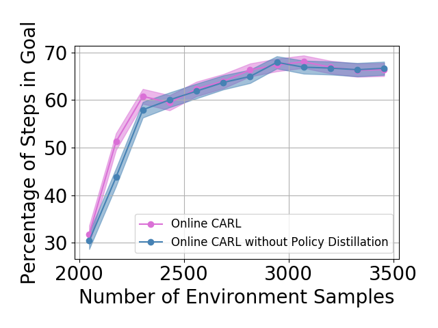
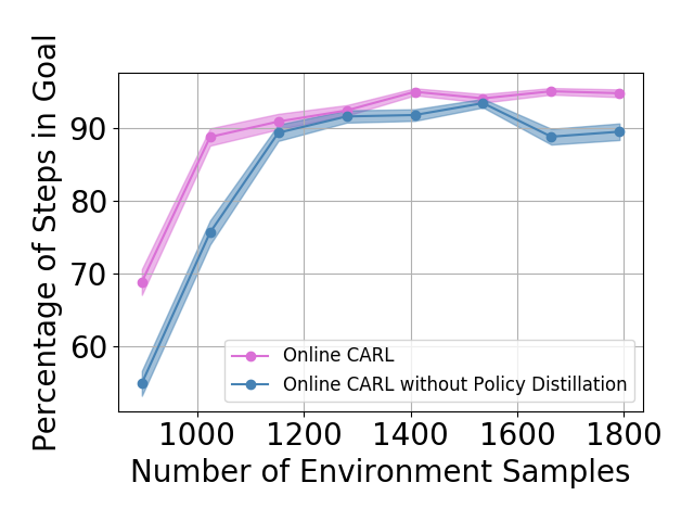
Policy Distillation In our iterative algorithm, we describe a method to connect policies from two different latent spaces in eq. (8). In Figure 5 we show the learning curves for Online CARL with and without policy distillation. In general, when utilizing policy distillation, we achieve similar performance to the iterative variant of our algorithm. Additionally, these results show that with policy distillation, in the three-pole and swingup tasks we are able to achieve faster convergence. Another observed added benefit is that with policy distillation we achieve more stability in the final metrics as we add more samples form our environment across environments.
Latent Representation and Performance for the Planar System All of the following figures were trained using the PCC framework. We present 5 representations with the worst control performance (Figure 6) and 5 representations that had the best control performance (Figure 7), with the PCC algorithm; thus we were using iLQR as the controller. Additionally, we present 5 representations that performed the worst (Figure 8) and 5 representations that performed the best (Figure 9) with our offline CARL algorithm; thus, we were using SAC as the controller. These maps were generated by uniformly sampling a state from the underlying environment, creating a corresponding observation , and using the encoder create the latent representation . All of the latent maps presented in Figures 6-9 are generated from the same PCC framework and same hyperparameters so the best performing maps are all fairly similar and the worst performing maps have similarities. It is important to note that even though these latent maps are similar, it is clear that their is a large difference in performance in table 3. Importantly, it is clear that iLQR struggles significantly more than SAC in these non-linear environments as seen in the worst case performance and the corresponding latent maps, where the latent maps contain additional twisting or curvature resulting in poorer performance.
In this case it is obvious that control in several of the latent representations that performed poorly would be difficult as there are regions that are highly non-smooth, non-locally-linear; thus, a locally linear controller such as iLQR is likely to perform poorly. We compare the top and worst 5 representations trained using the PCC framework, with the only difference being the controller (SAC vs. iLQR) in table 3.
| Environment | Algorithm | Worst 5 Avg. Results | Top 5 Avg. Results |
|---|---|---|---|
| Planar | PCC | ||
| Planar | Offline CARL | ||
| Swingup | PCC | ||
| Swingup | Offline CARL | ||
| Cartpole | PCC | ||
| Cartpole | Offline CARL | ||
| Three-pole | PCC | ||
| Three-pole | Offline CARL |
Additional SOLAR Results In our experiments for the planar, swingup, and cartpole environments we start from a point randomly chosen from a region surrounding the start point in the underlying MDP; additionally, in the planar case we randomize the target every episode. In Table 4, we present results where the start and goal states are from fixed points, to see if there is improvement in the SOLAR results. Also we try to shorten the horizon for swingup to to see if shorter horizons can play a factor in domains with rather long horizons. We don’t present any new results on the three-pole task as there was already a fixed starting state and fixed goal. We note that there is a dramatic improvement for the planar case when there is a fixed start and goal state and modest improvement in the cartpole and swingup cases. However, we still need to note that these results still are incomparable to the performance of any of CARL variants, offline CARL, online CARL, value-guided CARL, introduced in this paper.
| Environment | Algorithm | Number of Samples | Avg Result | Best Result |
|---|---|---|---|---|
| Planar | SOLAR | 5000 (VAE) + 40000 (Control) | ||
| Cartpole | SOLAR | 10000 (VAE) + 40000 (Control) | ||
| Swingup | SOLAR | 20000 (VAE) + 40000 (Control) |