Control and Simulation of Motion of Constrained Multibody Systems Based on Projection Matrix Formulation
Abstract
This paper presents a unified approach for inverse and direct dynamics of constrained multibody systems that can serve as a basis for analysis, simulation, and control. The main advantage of the dynamics formulation is that it does not require the constraint equations be linearly independent. Thus, a simulation may proceed even in the presence of redundant constraints or singular configurations and a controller does not need to change its structure whenever the mechanical system changes its topology or number of degrees of freedom. A motion control scheme is proposed based on a projected inverse-dynamics scheme which proves to be stable and minimizes the weighted Euclidean norm of the actuation force. The projection-based control scheme is further developed for constrained systems, e.g. parallel manipulators, which have some joints with no actuators (passive joints). This is complemented by the development of constraint force control. A condition on the inertia matrix resulting in a decoupled mechanical system is analytically derived that simplifies the implementation of the force control.
1 Introduction
Many robotic systems are formulated as multibody systems with closed-loop topologies, such as manipulators with end-effector constraints [1, 2, 3, 4, 5, 6, 7, 8, 9, 10, 11], cooperative manipulators [12, 13, 14, 15, 16], robotic hands for grasping objects [17, 18, 19, 20], parallel manipulators [21, 22, 23, 24], impact in robotics [25], humanoid robot and walking robots [26, 27, 28], and VR/Haptic applications [29, 30]. Simulation and control of such systems call for corresponding direct dynamics and inverse-dynamics models, respectively. Mathematically, constrained mechanical systems are modeled by a set of differential equations coupled with a set of algebraic equations, i.e. Differential Algebraic Equations (DAE). Although computing the dynamics model is of interest for both simulation and control, the research done in these two areas are rather divided. Surveys of the existing techniques for solving DAE may be found in [31, 32, 33, 34, 35, 29], while model-based control of constrained manipulators can be found in [4, 2, 36, 5, 37, 38, 39, 40, 41, 42, 43].
The classical method to deal with DAE is to express the constraint condition at the acceleration level. This allows replacement of the original DAE system with an ODE system by augmenting the inertia matrix with the second derivative of the constraint equation. However, this method performs poorly in the vicinity of singularities [44, 45, 46], because the augmented inertia matrix is invertible only with a full rank Jacobian matrix.
Other methods are based on coordinate partitioning [47, 48, 49] by using the fact that the coordinates are not independent because of the constraint equations. The motion of the system can be described by the independent coordinates which can be separated using an annihilator operator. Although this method may significantly reduce the number of equations, finding the annihilator operator is a complex task [29]. Moreover; the sets of independent and dependent coordinates should be determined first. But a fixed set of independent coordinates occasionally leads to ill-conditioned matrices [31, 50] when the system changes its topology or the number of degrees of freedom. The concept of coordinate separation is used in [9]for controlling manipulator robots with constrained end-effectors. The augmented Lagrangian formulation proposed in [51, 52, 53] can handle redundant constraints and singular situations. However, this formulation solves the equations of motion through an iterative process. Nakamura et al. [54] developed a general algorithm that provides a way to partition the coordinates into independent and dependent ones even around the singular configuration, which is suitable for simulation of mechanical systems with structure-varying kinematic chains. This is a special case of the projection method proposed herein that allows generic constraints which cannot be handled by coordinate partitioning.
There are also efficient algorithms for solving direct dynamics of constrained systems that are suitable for parallel processing. Feathersone’s work in [55, 56] presents a recursive algorithm, which is called Divide-and-Conquer (DAC), for calculating the forward dynamics of general rigid-body system on a parallel computer. The central formula for these DAC algorithm takes the equations of motions of two independent subassembly (rigid-body) and also a description of how they are to be connected, and the output is the equation of motion of the assembly, i.e., those of two articulated-body. Since the equation of acceleration of the assembly is written in terms of two independent equation of motions, the formulation is suitable for parallel processing and one can apply the formula recursively to construct the articulated-body equations of motions of an entire rigid-body assembly from those of its constituent parts. The author claims that the DAC algorithm is computationally effective if a large number of processors, more than , is available.
Another group of researchers [52, 57, 58, 46, 59, 60] focused on other techniques to deal with the problem of accurately maintaining the constraint condition. Blajer [58, 59] proposed an elegant geometric interpretation of constrained mechanical systems. Then the analysis was extended and modified in [61] for control application. The augmented Lagrangian formulation proposed in [51, 52, 53] can handle redundant constraints and singular situations. However, this formulation solves the equations of motion through an iterative process.
In the realm of control of constrained multibody system, the vast majority of the literature is devoted to control of manipulators with constrained end-effectors. The hybrid position/force control concept was originally introduced in [4], and then the manipulator dynamic model was explicitly included in the control law in [2]. The constrained task formulation with inverse-dynamics controller is developed in [5, 7] by assuming that the Cartesian constraints are linearly independent. Hybrid motion/force control proposed in [62, 63, 64] achieves a complete decoupling between channels of acceleration and force. In these approaches all joints are assumed to have an actuator and no redundancy was considered in the kinematic constraint.
In this work, we propose a new formulation for the direct and the inverse-dynamics of constrained mechanical systems based on the notion of a projection operator [1, 6]. First, constraint reaction forces are eliminated by projecting the initial dynamic equations into the tangent space with respect to the constraint manifold. Subsequently, the direct dynamics, or the equations of motion, is derived in a compact form that relates explicitly the generalized force to the acceleration by introducing a constraint inertia matrix, which turns out to be always invertible. The constraint reactions can then be retrieved from the dynamics projection in the normal space [1]. Unlike in the other formulations, the projection matrix is a square matrix of order equal to the number of dependent coordinates. Since the formulation of the projector operators is based on pseudo-inverting the constraint Jacobian (the process not conditioned upon the maximal rank of the Jacobian), the present approach is valid also for mechanical systems with redundant constraints and/or singular configurations, which is unattainable with many other classical methods. A projected inverse-dynamics control scheme is developed based on the dynamics formulation. The motion control proves to be stable while minimizing the weighted Euclidean norm of actuation force. The notion of the projected inverse-dynamics is further developed for control of constrained mechanical systems which have passive joints, i.e., joints with no actuator. This result is particulary important for control of parallel manipulators. Finally, a hybrid force/motion control scheme based on the proposed formulation is presented. Also some useful insights are gained from the dynamics formulation. For instance, the condition on the inertia matrix for achieving a complete decoupling between force and motion equations is rigorously derived.
This paper is organized as follows: We begin with the notion of linear operator equations in Section 2 by reviewing some basic definitions and elementary concepts which will be used in the rest of the paper. Using the projection operator, we derive models of inverse and direct dynamics in sections 4 and 5 which are used as a basis for developing strategies for simulation and control of constrained mechanical systems in sections 6 and 7. Section 7.2 presents change of coordinate if there is inhomogeneity in the spaces of the force and velocity. In section 7.4, the inverse-dynamics control scheme is extended for constrained systems which have some joints with no actuator (passive joints).
2 Linear Operator Equations
For any linear operator transformation , range space and null space are defined as and , respectively. The linear transformation maps vector space into vector space . Assume that the Euclidean inner-product is defined in , that is elements of vectors, such as and , of have homogeneous units. Then, by definition the vectors are orthogonal iff their inner-product is zero, i.e.
| (1) |
where the superscript T denotes transpose. It follows that the orthogonal complement of any set , denoted by , is the set of vectors each of which is orthogonal to every vector in .
Theorem 1
See Appendix A for a proof.
As will be seen in the following sections, it is desirable to be able to project any vector in to the null space of by a projector operator. Let be the orthogonal projection onto the null space, i.e., . Note that every orthogonal projection operator has these properties: and [66].
The projection operator can be calculated by the singular value decomposition (SVD) method [66, 67, 68]. Assuming
then there exist unitary matrices and (i.e. and ) so that
where , and are the singular values. The proof of this statement is straightforward and can be found, for example, in [66, 67]. Since [66, 67], the projection operator can be calculated by
| (4) |
2.1 Orthogonal Decomposition and Norm
From the definition, one can show that projector operator projects onto the null space orthogonal . Let’s assume that the elements of a vector have homogeneous measure units, then the vector has a unique orthogonal decomposition
where and . The components of the decomposition can be obtained uniquely by using the projection operator as
| (5) |
The Euclidean norm is defined as
| (6) |
Remark 1
From orthogonality of the subspaces, i.e. , we can say
| (7) |
Equation (7) forms the basis for finding an optimal solution.
2.1.1 Metric tensor
The Euclidean inner product and hence the Euclidean norm defined in (6) are non-invariant quantities, if there is inhomogeneity in the units of the elements of vector . With the same token, the projection matrix (5) and the decomposition are not invariant and hence the minimum-norm solution may depend on the measure units chosen. This is because components with different units are added together in (5).
To circumvent the quandary of the measure units, we consider the following transformation
| (8) |
and assume that the vector has components with the same physical units. Then, a physically consistent Euclidean inner product and Euclidean norm exists on the new space [63], i.e.
| (9) |
The symmetric, positive definite matrix is called a metric tensor of the n-space. Note that the Euclidean norm of the new coordinate is tantamount to the weighted-norm, that is , where
| (10) |
Furthermore, denoting , one can say . Let be the projection operator onto the null space of . Then, mapping is dimensionless and invariant.
3 Decomposition of the Acceleration
The kinematics of a constrained mechanical system can be represented by a set of nonlinear equations , where is the vector of generalized coordinate, and . Without loss of generality, we consider time-invariant (scleronomic) constraint conditions, but the methodology can be readily extended to a time varying case (rheonomic). By differentiating the constraint equation with respect to time, we have
| (11) |
where is the Jacobian of the constraint equation with respect to the generalized coordinate. For brevity of notation, in the following, we assume that the elements of the force and velocity vectors have homogeneous units. This assumption will be relaxed in Section 7.2 by changing of the coordinates similar to (8).
Equation (11) is expressed in form of the linear operation equation. This matrix equation specifies that any admissible velocity must belong to the null space of the Jacobian matrix, that is, . Thus, the constraint equation (11) can be expressed by the notion of the projection operator, i.e.,
| (12) |
Time differentiation of the above equation yields
| (13) |
where which, in turn, can be obtained from (4) by
| (14) |
It is apparent from equation (13) and (12) that, unlike the case of velocity, the null space orthogonal component of the acceleration is not always zero – a physical interpretation of (13) is given in Section 5.4. Equation (13) expresses the component of acceleration produced exclusively by the constraint and not by dynamics. As will be seen in Section 5, this equation can compliment the dynamics equation in order to provide sufficient independent equations for solving the acceleration.
3.1 Calculating based on Pseudo-Inversion
Many mature algorithms and numerical techniques are available for computing the pseudo-inverse [67, 66, 69]. There are also computer programs that can solve SVD and pseudo-inverse in real-time and non real-time, for instance DSP Blockset of Matlab [70]. Therefore, it may be useful to calculate the matrices and based on pseudo-inversion.
Let denote the pseudo-inverse of . Then, the projection operator can be calculated by
| (15) |
Also, one can obtain matrix through the pseudo-inversion as follows. Differentiation of (11) with respect to time leads to
The theory of linear systems of equations [66, 69, 71] establishes that the particular solution, i.e., the component of the acceleration, can be obtained from the above equation as . Hence
| (16) |
Assuming the elements of generalized coordinate have identical units, then matrices and have homogeneous units, i.e. is dimensionless and the dimension of is . Therefore, and are invariant under unit changes.
4 Projected Inverse-Dynamics
Consider a constrained mechanical system with Lagrangian , where and are the kinetic and the potential energy functions, and is the inertia matrix. The fundamental equation of differential variational principles of a mechanical system containing constraint can be written as [32]
| (17) |
where , , is the vector of generalized input force, and is the generalized constraint force, which is related to the Lagrange multipliers by
| (18) |
Then, the equations describing the system dynamics can be obtained as
| (19) |
| (20) |
where vector contains the Coriolis, centrifugal, gravitational terms. In solving the DAE equations (19)-(20), it is typically assumed that: (i) the inertia matrix is positive definite and hence invertible (ii) the constraint equations are independent, i.e. the Jacobian matrix is not rank-deficient [31, 32, 33, 34, 35, 29]. In this work, we solve the equations without relying on the second assumption.
From (18) and by virtue of Theorem 1, one can immediately conclude that . In other words, the projection operator is an annihilator for the constraint force, i.e. . Therefore, the constraint force can be readily eliminated from equation (19) if the equation is projected on , i.e.
| (21) |
Equation (21) is called projected inverse-dynamics of a constrained multibody system that is expressed in the so-called descriptive form. This is because matrix is singular and hence the acceleration cannot be computed from the equation through matrix inversion.
5 Direct Dynamics
As mentioned earlier, the acceleration cannot be determined uniquely from equation (21), because there are fewer independent equations than unknowns. Nevertheless; equations (13) and (21) are in orthogonal spaces and thus cannot cancel out each other. Therefore, a unique solution can be obtained by solving these two equations together. To this end, we simply multiply equation (13) by and then add both sides of the equation to those of (21). After factorization, the resultant equation can be written concisely in the following form;
| (22) |
where , and is called constraint inertia matrix which is related to the unconstrained inertia matrix —assuming a symmetric inertia matrix—by
| (23) |
and
| (24) |
Equation (22) constitutes the so-called direct dynamics of a constrained multibody system from which the acceleration can be solved. It is worth mentioning that if commutes with , then and hence . To compute the acceleration from (22) requires that the constraint inertia matrix be invertible.
Theorem 2
If the unconstrained inertia matrix is positive-definite (p.d.), then the constraint inertia matrix is p.d. too.
Proof: It is evident from (24) that is a skew-symmetric matrix, i.e. . Consequently, adding to the inertia matrix in equation (23) preserves the positive definiteness property of the inertia matrix. This is because, for any vector we can say
Therefore, one can conclude that , or
.
Theorem 2 is pivotal in showing the usefulness of the dynamics equation (22); it signifies that the constraint inertia matrix is always invertible regardless of the constraint condition. Therefore, the acceleration can be always obtained from (22).
Remark 2
Equation (22) signifies that only the null space component of the generalized input force contributes to the motion of a constrained mechanical system, as the projector in the right-hand-side (RHS) of the equation filters out all forces lying in the null space orthogonal. This fact is exploited in Section 7.1 for an optimal control scheme.
It can be envisaged from Remark 2 that it is useful to decompose the generalized input force into two orthogonal components
where and are called acting input force (potent) and passive input force (impotent), respectively. The decomposition of the generalized input force can be carried out by the projection operator according to (5). Now, the equation of motion can be written as
| (25) |
where the nonlinear vector is decomposed in the same way as the generalized force, i.e., . Equation (25) is the so-called equation of motion of a constrained mechanical system in a compact form. It is worth mentioning that only one matrix inversion operation is required in (25) which is one less than in the standard Lagrangian method (see Appendix B).
Remark 3
Since does not produce any kinetic energy, the total kinetic energy associated with the constrained system is .
5.1 Constraint Inertia Matrix
The constraint inertia matrix doesn’t have a unique definition because there are many ways that equations (21) and (13) can be combined together. Although all dynamics formulations thus obtained are equivalent, each one may have a ceratin computational advantage over the others.
5.1.1 Symmetric Inertia Matrix
is a p.d. matrix but not a symmetric one. In the following, we present an alternative dynamics formulation in which the inertia matrix appears both p.d. and symmetric. Equation (13) together with the decomposition of the acceleration imply that , which can be substituted in (21) to give
| (26) |
Now premultiply equation (13) by and then add both sides of the equation thus obtained with those of (26) yields
| (27) |
where
| (28) |
and
It is worth mentioning that represents a reflection operator.
Proposition 1
If matrix is symmetric and p.d., then is symmetric and p.d. too.
Proof: It is apparent from (28) that is a symmetric matrix . Moreover, positive definiteness of matrix can be shown by an argument similar to the previous case. Again for any vector and from definition (28), we can say , where and , and and . Both decomposed components of the non-zero vector cannot be zero, i.e., and vice versa. Therefore, only one of the quadratic functions can be zero and that implies their summation is non-zero and positive. Thus is a p.d. matrix .
5.1.2 Parameterized Inertia matrix
Alternatively, the constraint inertia matrix can be parameterized in terms of an arbitrary scalar. To this end, let’s first premultiply equation (13) by a scalar and then add both sides of the resultant equation with those of (21). That gives the standard dynamics formulation similar to (27) with the following parameters
| (29) |
and
Proposition 2
If is an invertible matrix, then is always invertible too.
Proof: In a proof by contradiction we show that should be a full-rank matrix. If matrix is not of full-rank, then there must exist at least one non-zero vector lying in the matrix null space, that is , or
| (30) |
The two terms of the above equation are in two orthogonal subspaces and cannot cancel out each other. Hence, in order to satisfy the equation, both terms must be identically zero, i.e. and . The former and the latter equations imply that and , respectively. Therefore, one can conclude that is perpendicular to vector , i.e. , or that
| (31) |
which is a contradiction because is a positive-definite matrix. Therefore, the null set of is empty and the matrix is always invertible, and this completes the proof .
Since is dimensionless, the scalar has the dimensions of mass. Therefore, the value of should be comparable to that of to avoid any numerical pitfall in the matrix inversion — a logical choice is ; yet, certain may lead to the minimum condition number of , which is desired for matrix inversion.
5.1.3 A Comparison of different Constraint Inertia Matrices
Theoretically, all the inverse-dynamics formulations presented here are equivalent, and they should yield the same result. However, from a numerical point of view, each has a certain advantage over the others that can lead to simplification of simulation or control. In summary,
-
•
is a p.d. matrix but not a symmetric one. If commutes with , then .
-
•
is a symmetric and p.d. matrix; hence it physically exhibits the characteristic of an inertia matrix. However, computing involves three additional matrix multiplication operations compared to .
-
•
is an invertible matrix, but it is neither p.d. nor symmetric. Nevertheless, computing of requires less computation effort compared to the others.
5.2 Constraint Force and Lagrange Multipliers
Equation (25) expresses the generalized acceleration of a constrained multibody system in a compact from without any need for computing the Lagrange multipliers. Yet, in the following we will retrieve the constraint force by projecting equation (19) onto , that gives
Now, substituting the acceleration from (25) into the above equation gives
| (32) |
where , and is the ratio of the two inertia matrices.
Equation (32) implies that the constraint force can always be obtained uniquely, but this may not be true for the Lagrange multipliers. Having calculated the constraint force from (32), one may obtain the Lagrange multipliers from equation (18) through pseudo-inversion, i.e., where is the homogeneous solution. By virtue of Theorem 1, we can also say that . This, in turn, implies that is a non-zero vector only if the Jacobian matrix is rank deficient, i.e. —recall that .
Remark 4
The vector of Lagrange multipliers can be determined uniquely iff the Jacobian matrix is full-rank. In that case, there is a one-to-one correspondence between and . Otherwise, the component of the Lagrange multiplies is indeterminate.
5.3 Decoupling
Fig.1 illustrates the input/output realization of a constrained mechanical system based on (25) and (32). The input channels and are the potent and the impotent components of the generalized input force, while the output channels are the acceleration and the constraint force, and , respectively. It is apparent form the figure that the acceleration is only affected by and not by whatsoever. However, the constraint force output, in general, can be affected by two inputs: by directly, and by through the cross-coupling channel . The cross-coupling channel is disabled if the inertia matrix satisfies a certain condition which is stated in Proposition 3.

Proposition 3
The equations of the constraint force and the acceleration are completely decoupled, i.e. the cross coupling vanishes if the null space of the constraint Jacobian is invariant under . That is, the inertia matrix should have this property: .
The proof is given in Appendix D.
Mechanical systems satisfying the condition in Proposition 3 are called decoupled constrained mechanical systems. The equation of constraint force of such a system is reduced to
In that case, the constraint force is determined exclusively by the passive input force that leads to a simple force control scheme, as will be seen in Section 7.3.
5.4 Illustrative Example and Geometrical Interpretation

A particle of mass moves on a circle of radius ; see Fig.2. Assume to be the generalized coordinate. The constraint equation is
which yields the Jacobian and its time-derivative as and , and the pseudo-inverse is . Then, from (15) we have
| (33) |
Let unit vectors and represent the tangential and normal directions as shown in Fig.2. Then, from (33) we have
The above equations represent the geometrical interpretation of the projection operators. Note that the normal component of the acceleration, , which can be interpreted as the Centripetal acceleration, is given by
| (36) | |||||
| (37) |
Let denote the external force applied on the particle. Observe that the decomposition of the force is aligned with the tangential and the normal directions to the circular trajectory shown in Fig.2. Finally, we arrive at the following set of dynamics equations:
6 Simulation of Constrained Multibody Systems
To simulate the dynamics of a constrained multibody system, one can make use of the acceleration model in (25). Having computed the generalized acceleration from the equation, one may proceed a simulation by integrating the acceleration to obtain the generalized coordinates. However, the integration inevitably leads to drift that eventually results in a large constraint error. Baumgarte’s stabilization term [35] is introduced to ensure exponential convergence of the constraint error to zero. However, this creates a very fast dynamics which tends to slow down the simulation. In this section, we use the pseudo-inverse for correcting the generalized coordinate in order to maintain the constraint condition precisely. It should be noted that using the pseudo-inverse here does not impose any extra computation burden, because the pseudo-inverse has to be obtained to compute the acceleration anyway.
Having obtained the velocity through integrating the acceleration, one may obtain the generalized coordinate by integration
| (38) |
where depicts integration time step. However, the constraint condition may be violated slightly because of integration drift. Let denote the coordinate after a few integration steps and . Now, we seek a small compensation in the generalized coordinate such that the constraint condition is satisfied: that is, a set of nonlinear equations must be solved in terms of . The Newton-Raphson method solves a set of nonlinear equations iteratively based on linearized equations.
The constraint equation can be written by the first order approximation as
Neglecting the term, one can obtain the solution of the linear system using any generalized inverse of the Jacobian. The pseudo-inverse yields the minimum-norm solution, i.e., . Therefore, the following loop
| (39) |
may be worked out iteratively until the error in the constraint falls into an acceptable tolerance, e.g. .
The condition for local convergence of multi-dimensional Newton-Raphson (NR) iteration can found, e.g., in [73, 74, 31]. Although it is known that NR iteration will not always converge to a solution, the convergence is guaranteed if the initial approximation is close enough to a solution [73, 74].
Theorem 3
[73] Assume that is differentiable in an open set , i.e., the Jacobian matrix exists, and that is Lipschitz continuous. Also assume that a solution exists, and that is nonsingular. Then under these assumptions, if the initial start point is sufficiently close to the solution, the convergence is quadratic, that is such that
One can expect that the drift, and hence the inial constraint error, can be reduced by decreasing the integration time step. It should be pointed out that the iteration loop (39) corrects the error in constraint coordinate caused by the integration process. Since the drifting error within a single integration time step is quite small, the initial estimate given by (38) cannot be far from the exact solution. Therefore, as shown by experiments, a fast convergence is achieved even though the iteration loop (39) is called once every few time steps.
Finally, the simulation of a constrained mechanical system based on the projection method can be proceeded in the following steps:
7 Control of Constrained Multibody Systems.
In this section we discuss the position and/or force control of constrained multibody systems based on the proposed dynamics formulation. The I/O realization of a constrained mechanical system is depicted in Fig.1, which will be used subsequently as a basis for development of control algorithm. In fact, the topology of a control system can be inferred from the figure by considering the decomposed components of the generalized input force, and , as the corresponding control inputs for position and force feedback loops.
Due to the decoupled nature of the acceleration channel, an independent position feedback loop can be applied. The input channel is directly transmitted to the constraint force, , and the velocity enters as a disturbance and hence must be compensated for in a feedforward loop. Note that in the case of decoupled mechanical systems, where the cross-coupling channel vanishes, exclusively determines the constraint force.
7.1 Motion Control Using Projected Inverse-Dynamics Control
Due to presence of only independent constraints, the actual number of degrees of freedom of the system is reduced to . Thus, in principle, there must be independent coordinates from which the generalized coordinates can be derived, i.e., . Now, differentiation of the given function with respect to time gives
| (40) |
| (41) |
where . Since constitutes a set of independent functions, the Jacobian matrix must be of full rank. (The proof is in Appendix E.). It is also important to note that any admissible function must satisfy the constraint condition, i.e.,
Using the chain-rule, one can obtain the time-derivative of the above equation
| (42) |
Since is a full-rank matrix, the only possibility for (42) to happen is that
| (43) |
Substituting the acceleration from (41) into the inverse-dynamics equation (21) gives the dynamics in terms of the reduced-dimensional coordinate
| (44) |
Let denote the desired trajectory of the new coordinates. Now, we propose the projected inverse-dynamics control (PIDC) law as follow
| (45) |
where is an auxiliary control input as
| (46) |
is the position tracking error, and and are the PD feedback gains. In the following, superscript is used to denote control input.
Theorem 4
Proof: Firstly, we prove exponential stability of the position error. From equations (44) – (46), one can conclude that the proposed control law leads to the following equation for the tracking error
| (47) |
To show that the expression within the bracket is zero, we need to show that the matrix is full-rank. In the following we will show that the matrix cannot have any null space and hence is full rank. If the matrix has a null space, then . Let us define . Recall that is a full-rank matrix and that —see (40). Hence, and . On other hand, implies that , and hence it is perpendicular to , i.e. . But, this is a contradiction because is a p.d. matrix. Consequently, , and it follows from (47) that
Hence, the error dynamics can be stabilized by selecting adequate gains, that is . Moreover, due to orthogonality of the decomposed generalized input force, we can say
From the above norm relation, it is clear that is the minimum norm solution, since any other solution must have a component in and this would increase the overall norm. Therefore, setting results in minimum norm of generalized input force subjected to producing the desired motion, i.e.,
| (48) |
7.2 Elements of Generalized Coordinate with Inhomogeneous Units
So far, we have assumed that the elements of the generalized velocity and the generalized input force have homogeneous units. Otherwise the minimum-norm solution of the generalized force, (48), makes no physical sense if the manipulator has both revolute and prismatic joints. In this section, we assume the vector of the generalized force to have a combination of force and torque components, and the vector of the generalized velocity with of rotational and translational components. As mentioned in Section 2.1.1, the minimization solution is not invariant with respect to changes in measure units if there is inhomogeneity of units in the spaces of the force and the velocity [75, 76]. To go around the quandary of inhomogeneous units, one can introduce a p.d. weight matrix by which the coordinates of the force vector is changed to
Note that the corresponding change of coordinates for the velocity is in order to preserve the force-velocity product (by virtue of (17)). Therefore, the metric tensors for the force and velocity vectors are and , respectively. The inertia matrix and the Jacobian with respect to the new coordinates are and . Since and and the corresponding projection matrix , where , is always dimensionless and, hence, invariant under the measure units chosen. The new force and velocity vectors have homogeneous units if the weight matrix is properly defined. Therefore, replacing the new parameters, which are now dimensionally consistent, in the optimal control (45) minimizes or equivalently minimizes the weighted Euclidean norm of the generalized input force, i.e.,
| (49) |
A quiet direct structure for is the diagonal one, i.e.,
| (50) |
where is a length, by which we divide the translational-velocity (or multiply the force). Using this length is tantamount to the weighted norm as
where the added terms are homogeneous, and and are the force and the torque components of . It is worth pointing out that a characteristic length that arises naturally in the analysis and leads to invariant results was proposed in [77, 78].
Alteratively, the weight matrix can be selected according to some engineering specifications. For instance, assume that the maximum force and torque generated by the actuators are limited to and . Then, choosing leads to the minimization of this cost function
which, in a sense, takes the saturation of the actuators into account.
7.3 Control of Constraint Force
The motion controller proposed in 7.1 works well for mechanical systems with bilateral constraint. On the other hand, since the proposed controller doesn’t guarantee that the sign of the constraint force will not change, a unilateral constraint condition may not be physically maintained under the control law. In this case, controlling the constraint force is a necessity.
Suppose that represents desired constraint force which can be derived from the desired Lagrange multipliers using
Then, considering as a control input, we propose the following control law
| (51) |
where is the auxiliary control input which is traditionally chosen as
| (52) |
in which is the force error, and and are the PI feedback gains. It should be pointed out that the integral term is not necessary, but it improves the steady-state error. From (32), (51), and (52), one can obtain the error dynamics as
which will be stable provided that the gains are positive definite, i.e., as . Define , and . Then,
| (53) |
where is the minimum singular value of the Jacobian, i.e.,
Therefore, one can conclude tracking of the Lagrange multipliers, i.e. as , if the Jacobian is full rank or .
Remark 5
The constraint force is always controllable, while the Lagrange multipliers are controllable only if the Jacobian matrix is of full rank.
It is worth mentioning that, unlike the traditional motion/force control schemes, which lead to coupled dynamics of force error and position error, our formulation yields two independent error equations. This is an advantage, because the motion control can be achieved regardless of the force control and vice versa. To this end, a hybrid motion/force control law can be readily obtained by combining (45) and (51),
7.4 Control of Constrained Mechanical Systems with Passive Joints
Some constrained mechanical systems, e.g., parallel manipulators, have joints without any actuators. The joints with and without actuators are called active joints and passive joints, respectively. In this section, we use the notion of the linear projection operator to generalize the inverse-dynamics control scheme for constrained mechanical systems with passive joints. Assuming there are active joints (and passive joints), the generalized input force has to have this form
This implies that any admissible generalized force should satisfy
| (55) |
where is a identity matrix. Note that is a projection onto the actuator space , i.e., and .
Now, we need to modify the motion control law (45) so that the condition in (55) is fulfilled. If , then (55) is automatically satisfied by choosing . Otherwise, we need to add a component, say , to so that . Since does not affect the system motion at all, the motion tracking performance is preserved by that enhancement—albeit control of constraint force may no longer be achievable. Let us assume
| (56) |
where . Then, we seek such that
| (57) | |||||
where . Consider as the unknown variable in (57). A solution exits if the RHS of (57) belongs to the range of , i.e.,
| (58) |
Then, the particular solution can be found via pseudo-inversion, i.e.,
| (59) |
The above equation yields the minimum-norm solution, i.e., minimum , which eventually minimizes the actuation force. Equations (56) and (59) give
| (60) |
where
| (61) |
Finally, we arrive at the following control law for constrained mechanical systems with passive joints
| (62) |
with derived from (45).
7.4.1 Minimum-norm Torque
7.4.2 Controllability
Because the existence of a solution is tantamount to the controllability condition of constrained mechanical systems under the proposed control law, it is important to find out when a solution to (57) exists, It can be inferred from (58) that
| (64) |
In general, the proposed control method for systems with passive joints works only if there exist sufficient number of active joints. Since occurrence of the singularities gives rise to the number of dof, the system under control law may no longer be controllable if there are not enough active joints. For instance, mechanical systems without any constraints at all cannot be controlled unless all joints are actuated. This is because no-constraint means that or ; hence, according to (64), a controllable system requires that , which means there can be no passive joints.
Also, it is worth pointing out that choosing trivially results in a controllable system.
8 A Slider-Crank Case Study
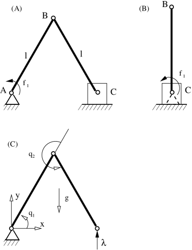
In this section, we describe the results obtained from applying the proposed inverse and direct dynamics formulations for simulation and control of a slider-crank mechanism, Fig.3A. Assume that the dimension of the crank and the connecting rod are the same. Then, singular configurations occur at
| (65) |
see Fig.3B.
8.1 Equations of Direct Dynamics
As shown in Fig.3C, the closed-loop is cut in the right hand support, i.e., at joint C. Let’s vector denote the joint angles. Then, the vertical position of the point C is
| (66) |
where is the length of linkage. In the sequel, ,,, are shorthanded for , , , and according to the notation in [79]. The vertical translation motion of point C is prohibited by imposing the following scleronomic constraint equation
| (67) |
Now, derivation of the direct dynamics may proceed as the following steps:
Step 1: Obtain the dynamic parameters of the open chain system Fig.3C (this is similar to the two-link manipulator case study in [79]) as
| (68) |
where represent the mass of the link.
Step 2: Compute the projection matrix corresponding to the constraint equation (67). The Jacobian of the constraint is
| (69) |
The projection matrix can be computed numerically (e.g. using the SVD of DSP Blockset in Matlab/Simulink [70]). Nevertheless, we obtain in a closed form for this particular illustration to have some insight into how the SVD handles singularities. Since , the Jacobian matrix (69) can be simplified as whose singular value is trivially . The SVD algorithm treats all singular values less that as zeros, i.e., if . Hence
| (70) |
This indicates the constraint is virtually removed if the system is sufficiently closed to the singular configurations (65).
Conclusion
A unified formulation applicable to both the direct dynamics (simulation) and inverse-dynamics (control) of constrained mechanical systems has been presented. The approach is based on projecting the Lagrangian dynamic equations into the tangent space with respect to the constraint manifold. This automatically eliminates the constraint forces from the equation, albeit the constraint forces can be then retrieved separately from dynamics projection into the normal space.
The novelty of the formulation lies in the definition of the projector operators which, unlike in the other formulations, are square matrices of order equal to the number of dependent coordinates. Therefore, the structure of the dynamics formulation doesn’t change if the system changes its degree-of-freedom or its topology. Moreover, since the process of computing projection operator is not conditioned upon the maximal rank of the Jacobian, the direct and the inverse-dynamics formulation are valid also for mechanical systems with redundant constraints and/or singular configurations, which is unattainable with many other classical approaches.
A motion control system has been developed based on the projected inverse-dynamics control which, minimizes actuation force, and also works for systems having unactuated joints (passive joints). To this end, a hybrid motion/force controller was developed.
In summary, particular features of the proposed formulation associated with simulation and control of constrained mechanical systems are listed below:
-
•
A simulation may proceed even with presence of redundant constraint equations and/or singular configurations. With the same token, the projected inverse-dynamics motion controller can cope with changes in the system’s constraint topology or number of degrees-of-freedom.
-
•
The generalized formulation requires no knowledge of the constraint topology, i.e., description of how subassemblies are connected, and it works for rigid-body or flexible systems alike.
-
•
The inverse-dynamics control scheme leads to minimum weighted Euclidean norm of control force input.
-
•
The inverse-dynamics control scheme can be applied for constrained systems which has some joints with no actuator.
-
•
If the inertia matrix posses a certain property as stated in Proposition 3, the system exhibits decoupling which leads to further simplification of the force control.
-
•
Redundant and flexible manipulators can be dealt with.
Appendix A
Appendix B
Assuming that the Lagrange multipliers is known, the acceleration can be carried out from equation (19)
| (74) |
Substituting the acceleration from (74) into the second differentiation of the constraint equation
gives the Lagrange multipliers as
| (75) |
This methods works only if the Cartesian inertia matrix is not singular. Finally, substituting (75) to (74) yields the acceleration.
Appendix C
Lemma 1
The subspace is invariant under an invertible transformation if and only if the subspace is invariant under .
Proof: By definition, is an invariant subspace under iff . Moreover, the invertible mapping cannot reduce the dimension of any subspace, that is , hence . It follows
which completes the proof .
Appendix D
It is apparent from Fig.1 that the decoupling is achieved iff
| (76) |
which implies the null space must be invariant under . Since is an invertible mapping, it can be inferred from Lemma 1 (see Appendix C) that the null space must be invariant under too. Thais means that (76) is equivalent to . Now, replacing from (23) into the latter equation and after factorization, one can infer the followings
| decoupling | ||||
which completes the proof.
Appendix E
Since is a set of independent functions, the corresponding Jacobian matrix is full rank, i.e., . Moreover, by using the chain-rule, we have , where is a identity matrix. Now, by virtue of the property of the rank operator 111, one can say
or
References
- [1] F. Aghili, “A unified approach for inverse and direct dynamics of constrained multibody systems based on linear projection operator: Applications to control and simulation,” IEEE Trans. on Robotics, vol. 21, no. 5, pp. 834–849, Oct. 2005.
- [2] O. Khatib, “A unified approach for motion and force control of robot manipulators: The operational space formulation,” vol. RA-3, no. 1, pp. 43–53, 1987.
- [3] F. Aghili and K. Parsa, “A reconfigurable robot with lockable cylindrical joints,” IEEE Trans. on Robotics, vol. 25, no. 4, pp. 785–797, August 2009.
- [4] M. H. Raibert and J. J. Craig, “Hybrid position/force control of manipulators,” ASME Journal of Dynamic Systems, Measurement, and Control, vol. 102, pp. 126–133, Jun. 1981.
- [5] T. Yoshikawa, “Dynamic hybrid position/force control of robot manipulators-description of hand constraints and calculation of joint driving force,” vol. RA-3, no. 5, pp. 386–392, Oct. 1987.
- [6] F. Aghili, “Inverse and direct dynamics of constrained multibody systems based on orthogonal decomposition of generalized force,” in IEEE Int. Conf. on Robotics & Automation, Taipei, Taiwan, 2003, pp. 4035–4041.
- [7] T. Yoshikawa, T. Sugie, and M. Tanaka, “Dynamic hybrid Position/Force control of robot manipulators – controller design and experiment,” IEEE J. of Robotics and Automation, vol. 4, pp. 699–705, 1988.
- [8] J.-C. Piedbœuf, J. de Carufel, F. Aghili, and E. Dupuis, “Task verification facility for the Canadian special purpose dextrous manipulator,” in IEEE Int. Conf. on Robotics & Automation, Detroit, Michigan, May 10–15 1999, pp. 1077–1083.
- [9] N. H. McClamroch and D. Wang, “Feedback stabilization and tracking in constrained robots,” IEEE Trans. on Automation Control, vol. 33, pp. 419–426, 1988.
- [10] F. Aghili and J.-C. Piedbœuf, “Simulation of motion of constrained multibody systems based on projection operator,” Journal of Multibody System Dynamics, vol. 10, pp. 3–16, 2003.
- [11] F. Aghili and J.-C. Piedboeuf, “Emulation of robots interacting with environment,” IEEE/ASME Trans. on Mechatronics, vol. 11, no. 1, pp. 35–46, Feb. 2006.
- [12] Y. R. Hu and A. A. Goldenberg, “Dynamic control of coordinated redundant robots with torque optimization,” vol. 29, no. 6, 1993.
- [13] M. Namvar and F. Aghili, “Adaptive force-motion control of coordinated robots interacting with geometrically unknown environments,” IEEE Trans. on Robotics, vol. 21, no. 4, pp. 678–694, Aug. 2005.
- [14] J. H. Jean and L. C. Fu, “An adaptive control scheme for coordinated multimanipulator systems,” IEEE Trans. Robotics and Automation, vol. 9, no. 2, pp. 226–231, 1993.
- [15] F. Aghili, “Adaptive control of manipulators forming closed kinematic chain with inaccurate kinematic model,” IEEE/ASME Trans. on Mechatronics, vol. 18, no. 5, pp. 1544–1554, October 2013.
- [16] M. Namvar and F. Aghili, “Adaptive control of cooperative robots interacting with a geometrically unknown environment,” in IEEE Int. Conference on Robotics & Automation, New Orleans, USA, 2004.
- [17] F. Aghili, “Robust impedance control of manipulators carrying heavy payload,” ASME Journal of Dynamic Systems, Measurements, and Control, vol. 132, September 2010.
- [18] A. B. A. Cole, J. E. Hauser, and S. S. Sastry, “Kinematics and control of multifingered hands with rolling contact,” IEEE Transactions on Automatic Control, vol. 34, no. 4, pp. 398–404, Apr 1989.
- [19] F. Aghili, “A prediction and motion-planning scheme for visually guided robotic capturing of free-floating tumbling objects with uncertain dynamics,” IEEE Transactions on Robotics, vol. 28, no. 3, pp. 634–649, June 2012.
- [20] X. Z. Zheng, R. Nakashima, and T. Yoshikawa, “On dynamic control of finger sliding and object motion in manipulation with multifingered hands,” IEEE Trans. Robotics and Control, vol. 16, pp. 469–481, 2000.
- [21] F. Aghili, “Projection-based control of parallel mechanisms,” ASME Journal of Computational and Nonlinear Dynamics, vol. 6, no. 3, July 2011.
- [22] J. J. Murray and G. H. Lovell, “Dynamic modeling of closed-chain robotic manipulators and implications for trajectory control,” IEEE Trans. Robotics and Automation, vol. 5, pp. 522–528, 1989.
- [23] F. Aghili, “Modelling and analysis of multiple impacts in multibody systems under unilateral and bilateral constrains based on linear projection operators,” Multibody Syst. Dyn., vol. 46, no. 1, pp. 41–62, 2019.
- [24] Y. Nakamura and M. Ghodoussi, “Dynamics computation of closed-link robot mechanism with nonredundant actuators,” IEEE Trans. Robotics and Automation, vol. 5, pp. 294–302, 1989.
- [25] F. Aghili, “Energetically consistent model of frictional impacts in multibody systems in sticking and sliding modes,” Multibody Syst. Dyn., Jan. 2019.
- [26] B. Perrin, C. Chevallereau, and C. Verdier, “Calculation of the direct dynamics model of walking robots: Comparison between two methods,” in IEEE Int. Conf. Robotics and Automation, Apr. 1997, pp. 1088–1093.
- [27] D. Surla and M. Rackovic, “Closed-form mathematical model of dyanmics of anthropomorphic locomotion robot mechnism,” in In Proceedings of 2nd ECPD Int. Conf. Adv. Robotics, Intell. Automat. Active Syst., 1996, pp. 327–331.
- [28] F. Aghili, “Quadratically constrained quadratic-programming based control of legged robots subject to nonlinear friction cone and switching constraints,” IEEE/ASME Transactions on Mechatronics, vol. 22, no. 6, pp. 2469–2479, Dec 2017.
- [29] A. Bicchi, L. Pallottino, M. Bray, and P. Perdomi, “Randomized parrallel simulation of constrained multibody systems for VR/Haptic applications,” in IEEE Int. Conference on Robotics and Automation, Seoul, Korea, 2001, pp. 2319 – 2324.
- [30] F. Aghili, “Robust impedance-matching of manipulators interacting with uncertain environments: Application to task verification of the space station’s dexterous manipulator,” IEEE/ASME Transactions on Mechatronics, vol. 24, no. 4, pp. 1565–1576, Aug 2019.
- [31] J. Garcia de Jalón and E. Bayo, Kinematic and Dynamic Simulation of Multibody Systems: The Real-Time Challenge. New York: Springer-Verlag, 1994.
- [32] J. G. de Jalon and E. Bayo, Kinematic and Dynamic Simulation of Multibody Systems. Springer-Verlag, 1989.
- [33] U. M. Ascher and L. R. Petzold, “Computer methods for ordinary differential equations and differential-algebraic equations,” SIAM, 1998.
- [34] C. W. Gear, “The simultaneous numerical solution of differential-algebraic equations,” IEEE Trans. Circuit Theory, vol. CT-18, pp. 89–95, 1971.
- [35] J. Baumgarte, “Stabilization of constraints and integrals of motion in dynamical systems,” vol. 1, pp. 1–16, 1972.
- [36] F. Aghili, “Projection-based modeling and control of mechanical systems using non-minimum set of coordinates,” in Proc. of IEEE/RSJ International Conference on Intelligent Robots and Systems (IROS), Hamburg, Germany, Sep. 2015, pp. 3164–3169.
- [37] F. Aghili, “Control of redundant mechanical systems under equality and inequality constraints on both input and constraint forces,” ASME Journal of Computational and Nonlinear Dynamics, vol. 6, no. 3, July 2011.
- [38] N. Hogan, “Impedance control an approach to manipulation: Part i - theory,” Journal of Dynamic Systems, Measurement, and Control, vol. 107, pp. 1–7, 1985.
- [39] H. West and H. Asada, “A method for the design of hybrid position/force controllers for mainpulatros constrained by contact with environment,” in IEEE Int. Conf. Robotics and Automation, St. Louis, MO, Mar. 1985, pp. 251–259.
- [40] F. Aghili, “A unified approach for control of redundant mechanical systems under equality and inequality constraints,” in Proc. of IEEE/RSJ International Conference on Intelligent Robots and Systems (IROS), Taipei, Taiwan, Oct. 2010, pp. 4849–4854.
- [41] S. Chiaverini and L. Sciavicco, “The parallel approach to force/position control of robotic manipulators,” IEEE Trans. on Robotics and Automation, vol. 9, pp. 361–373, 1993.
- [42] C. Canudas de Wit, B. Siciliano, and G. Bastin, Eds., Theory of Robot Control. London, Great Britain: Springer, 1996.
- [43] F. Aghili, “Self-tuning cooperative control of manipulators with position and orientation uncertainties in the closed-kinematic loop,” in Proc. of IEEE/RSJ International Conference on Intelligent Robots and Systems (IROS), San Francisco, CA, Sep. 2011, pp. 4187–4193.
- [44] C. O. Chang and P. E. Nikravesh, “An adaptive constraint violation stabilization method for dynamic analysis of mechanical systems,” Journal of Mechanisms, and Automation in Design, vol. 107, pp. 488–492, 1985.
- [45] S. T. Lin and M. C. Hong, “Stabilization method for numerical integration of multibody mechanical systems,” Journal of Mechanical Design, vol. 120, pp. 565–572, 1998.
- [46] S. Yoon, R. M. Howe, and D. T. Greenwood, “Stability and accuracy analysis of baumgarte’s constraint violation stabilization method,” Journal of Mechanical Design, vol. 117, pp. 446–453, 1995.
- [47] R. A. Wehage and E. J. Haug, “Generalized coordinate partitioning for dimension reduction in analysis of constrained dynamic systems,” ASME J. Mech. Design, vol. 104, pp. 247–255, 1982.
- [48] P. E. Nikravesh and I. S. Chung, “Application of euler parameters to the dynamic analysis of three dimensional constrained mechanical systems,” ASME J. Mech. Design, vol. 104, pp. 785–791, 1982.
- [49] C. G. Liang and G. M. Lance, “A differentiable null space method for constrained dynamic analysis,” Trans. ASME, JMTAD, vol. 109, pp. 450–411, 1987.
- [50] W. Blajer, W. Schiehlen, and W. Schirm, “A projective criterion to the coordinate partitioning method for multibody dynamics,” Applied Mechanics, vol. 64, pp. 86–98, 1994.
- [51] E. Bayo and J. G. de Jalon, “A modified lagrangian formulation for the dynamic analysis of constrained mechanical systems,” vol. 71, pp. 183–195, 1988.
- [52] E. Bayo and R. Ledesma, “Augmented lagrangian and mass-orthogonal projection methods for constrained multibody dynamics,” vol. 9, pp. 113–130, 1996.
- [53] J. Cuadrado, J. Cardenal, and E. Bayo, “Modeling and solution methods for efficient real-time simulation of multibody dynamics,” vol. 1, pp. 259–280, 1997.
- [54] Y. Namamura and K. Yamane, “Dynamics computation of structure-varying kinematic chains and its application to human figures,” IEEE Trans. On Robotics and Automation, vol. 16, pp. 124–134, 2000.
- [55] R. Featherstone, “A divide-and-conquer articulated-body algorithm for parallel o(log(n)) calculation of rigid-body dynamics. part 1 &,” vol. 18, no. 9, pp. 867–875, 1999.
- [56] R. Featherstone and D. Orin, “Robot dynamics: Equations and algorithms,” in IEEE Int. Conf. On Robotics & Automation, San Francisco, CA, 2000, pp. 826–834.
- [57] K. C. Park and J. C. Chiou, “Stabilization of computational procedures for constrained dynamical systems,” Jounal of Guidance, Control and Dynamics, vol. 11, pp. 365–370, 1988.
- [58] W. Blajer, “A geometric unification of constrained system dynamics,” Multibody System Dynamcis, vol. 1, pp. 3–21, 1997.
- [59] W. Blajer, “Elimination of constraint violation and accuracy aspects in numerical simulation of multibody systems,” vol. 7, pp. 265–284, 2002.
- [60] F. Aghili, “Non-minimal order model of mechanical systems with redundant constraints for simulations and controls,” IEEE Transactions on Automatic Control, vol. 61, no. 5, pp. 1350–1355, May 2016.
- [61] L. Guanfeng and L. Zexiang, “A unified geometric approach to modeling and control of constrained mechanical systems,” IEEE Trans. Robotics and Automation, vol. 18, pp. 574–587, 2002.
- [62] A. D. Luca and C. Manes, “Modeling of robots in contact with a dynamic environment,” IEEE Trans. on Robotics & Automation, vol. 10, no. 4, pp. 542–548, 1994.
- [63] K. L. Doty, C. Melchiorri, and C. Bonivento, “A theory of generalized inverses applied to robotics,” vol. 12, no. 1, pp. 1–19, 1993.
- [64] J. D. Schutter and H. Bruyuinckx, The Control Handbook. New York: CRC, 1996, ch. Force Control of Robot Manipulators, pp. 1351–1358.
- [65] C. Desoer, Notes for a Second Course on Linear Systems. Van Nostrand Reinhold, 1970.
- [66] G. H. Golub and C. F. V. Loan, Matrix Computations. Baltimore and London: The Johns Hopkins University Press, 1996.
- [67] W. H. Press, B. P. Flannery, S. A. Teukolsky, and W. T. Vetterling, Numerical Recipies in C: The Art of Scientific Computing. NY: Cambridge University Press, 1988.
- [68] C. Belta and V. Kumar, “An SVD-based projection method for interpolation on SE(3),” IEEE Trans. on Robotics and Automation, vol. 18, no. 3, pp. 334–345, Jun. 2002.
- [69] A. Ben-Israel and T. N. E. Greville, Generalized Inverse: Theory and Applications. New York: Robert E. Krieger, 1980.
- [70] DSP Blockset for Use with Simulink, User’s Guide, The MathWorks Inc., 24 Prime Parlway, Natick, MA 011760-1500, 1998.
- [71] Y. Nakamura, Advanced Robotics: Redundancy and Optimization. Reading, Massachusetts: Addison-Wesley Publishing Company, 1991.
- [72] W. Blajer, “A geometrical interpretation and uniform matrix formulation of multibody system dynamics,” vol. 81, no. 4, pp. 247–259, 2001.
- [73] C. T. Kelly, Iterative Methods for Linear and Nolinear Equations. Philadelphia: SIAM, 1995.
- [74] M. Honkala and M. Valtonen, “New multilevel newton-raphson method for parallel circut simulation,” in European Conference on Circut Theory and Design, ECCTD, Espoo, Finland, Aug. 2001.
- [75] H. Lipkin and J. Duffy, “Hybrid twist and wrench control for a robotic manipulator,” Trans. ASME J. of Mechanism, Transmission, and Automation in Design, vol. 110, pp. 138–144, 1988.
- [76] C. Manes, “Recovering model consistence for force and velocity measures in robot hybrid control,” in IEEE Int. Conference on Robotics & Automation, Nice, France, 1992, pp. 1276–1281.
- [77] J. Angeles, Fundamentals of Robotic Mechanical Systems. Theory, Methods, and Algorithms, New York, 1997.
- [78] ——, “A methodology for the optimum dimensioning of robotic manipulators.” UASLP, San Luis Potosí, SLP, México: Memoria del 5o. Congreso Mexicano de Robótica, 2003, pp. 190–203.
- [79] J. J. Craig, Introduction to Robotics: Mechanical and Control, 2nd ed. Reading, Massachusetts: Addison-Wesley Publishing Company, 1989.