Control Ability with Time Attributy for Linear Continous-time Systems ††thanks: Work supported by the National Natural Science Foundation of China (Grant No. 61273005)
Abstract
In this paper, the control ability with time attributy for the linear continuous-time (LCT) systems are defined and analyzed by the volume computing for the controllability region. Firstly, a relation theorem about the open-loop control ability, the control strategy space (i.e., the solution space of the input variable for control problems), and the some closed-loop performance for the LCT systems is purposed and proven. This theorem shows us the necessity to optimize the control ability for the practical engineering problems. Secondly, recurssive volume-computing algorithms with the low computing complexities for the finite-time controllability region are discussed. Finally, two analytical volume computations of the infinite-time controllability region for the systems with different and repeated real eigenvalues are deduced, and then by deconstructing the volume computing equations, 3 classes of the shape factors are constructed. These analytical volume and shape factors can describe accurately the size and shape of the controllability region. Because the time-attribute control ability for LCT systems is directly related to the controllability region with the unit input variables, based on these analytical expressions on the volume and shape factors, the time-attribute control ability can be computed and optimized conveniently.
keywords:
control ability , controllability region , smooth geometry , volume computation , shape factor , continuous-time systems , state controllability , state reachability1 Introduction
The concepts of the state controllability and observability for the dynamical systems, born in 1960’s by R. Kalman, et al, [13] became the firm basises of many branches of control theory, such as optimal control, stochastic control, nonlinear control, adaptive control, robust control, . The so-called state controlabiity is only a two-values logic concept whether the states in state space can be controlled or not by the input variables of the dynamical systems, and the state observability is also a two-values logic concept whether the unmeasurable states can be estimated or not by the measurable output and input variables. The controllability concepts and corresponding criterions can tell us that the dynamical systems are controllable or not, and but the control ability and control effciency can not be analyzed and got. So is observability. In fact, the quantitative concept and analysis methods for that are very important for the practical control engineering, and many control engineering problems are dying to these quantitative studies.
In past 60 years, some works stated as follows are on the quantitation of control ability.
1) Based the definition of the controllability Grammian matrix and the correspongding controllability Ellipsoid , in papers [16], [6], [15], and [11], the determinant value and the minimum eigenvalue of the matrix , correspondingly the volume and the minimum radius of the ellipsoid , can be used to quantify the control ability of the input variable to the state space, and then be chosen as the objective function for optimizing and promoting the control ability of the linear dynamical systems. Due to lack of the analytical computing of the determinant and eigenvalue , correspondingly the volume and the radius , these optimizing problems for the control ability are solved very difficulty, and few achievements about that have been made.
2) Based the definition of the controllability region , the minimum distance of the boundary to the original of the state space is used to measure and optimize the control ability [17]. Because of the difficulty to compute the distance, the further works have not been reported.
3) Based on the well-known PBH controllability test, a degree of modal controllability was put forward to measure and optimize the control ability with the eigenvalue mobility, i.t., the changing ability of the system eigenvalues by the control law [14] [7] [8]. Because the degree is only for the single modal and not for the whole system, the further works have not been carried forward.
Recently, a systemical studies on the control ability of the input variables to the state variables for the linear discrete-time (LDT) systems are carried out by M.W. Zhao [20] [18] [21] [19], a new quantifying concept and analysis method for the control ability are put forth. And then a relation theorem among the open-loop control ability, the control strategy space (i.e., the solution space of the input variables for the control problems), and the some closed-loop control performance, such as, the optimal time waste, the response speed, the robustness of the the control strategy, , is purposed and proven in paper [21]. By the theorem in paper [21], we can see, optimizing the control ability of the open-loop systems is with the great significations for promoting the performance indices of the closed-loop control systems. In addtion, in these papers, the analytical expressions of the volumes and the multiple shape factors of the controllability region/ellipsoid are deduced and can be used to analyze and optimize the control ability. Based on these results, the analysis and optimization methods for the control ability of the LDT systems can be founded.
In this paper, the concepts and analysis methods for control ability of the LDT systems in [20] [21] [19] will be generalized to the linear continuous-time (LCT) systems, and it is expected that the analyzing and optimizing for the time-attribute control ability of LCT systems can be carried out conveniently based on the new results in this paper.
2 Definition on the Control Ability with Time Attribute
In general, the LCT Systems can be modelled as follows:
| (1) |
where and are the state variable and input variable, respectively, and matrices and are the state matrix and input matrix, respectively [12] [3]. To investigate the controllability of the LCT systems (1), the controllability matrix and the controllability Grammian matrix can be defined as follows
| (2) | ||||
| (3) |
That the rank of the matrix / is , that is, the dimension of of the state space the systems (1), is the well-known criterion on the state controllability.
In papers [16], [6], [15], and [11], the determinant value and the minimum eigenvalue of the controllability Grammian matrix can be used to quantify the control ability of the input variable to the state space, and then be chosen as the objective function for optimizing and promoting the control ability of the linear dynamical systems. Due to lack of the analytical computing of the determinant and eigenvalue , these optimizing problems for the control ability are solved very difficulty, and few achievements about that were made. Out of the need of the practical control engineering, quantifying and optimizing the control ability are key problems in control theory and engineering fields, and the further studyings on that are encouraged.
2.1 The Normalization of the Input Variable and The Definitions of the Controllability Region
According to paper [21], to study rationally the control ability of the input variables to the state variables for the different dynamical systems, it is necessary to normalize the input variable and state variables. For studying the control ability with time attribute, the normalization of the input variablles is as follows
| (4) |
where and are the input variable numbers and the -th input variable of the multi-input systems, respectively. In fact, the constraint condition (4) can be used to describe the input variables for the following two cases:
1) The input variables are bounded or with some saturation elements.
2) The unit input variables are considered for conveniently computing and comparing the control ability.
Based on the above normolization on the input variables, the state controllability region and control ability with time attribute can be defined and studied. In this paper, the controllability region is a broad concept and it includes narrow controllability region and reachability region. The so-called narrow controllability region and reachability region are the state ranges of the controllable state and reachable state, respectively. The word ’controllable state’ means the state that can be controlled to the original of the state space by a finite-time input sequence, and ’reachable state’ means the state that can be reached form the original by a finite-time input sequence.
Similar to the definition of the state controllability region ( a.k.a. ”recover region”) for the input-saturated linear systems in papers [1], [9], [10], the narrow controllability region and reachability region of the LCT Systems with the input constraints are defined as follows
| (5) | ||||
| (6) |
In fact, the controllability regions and reachability region are the biggest range of the controllable states and the reachable states with the unit input variables.
In paper [20], a special zonotope generated by the matrix pair is defined as follows
| (7) |
and the controllability region of the LDT systems can be regarded as a special zonotope defined as (7). Similarly, a smooth geometry generated by the matrix pair can be defined as follows
| (8) |
Similar to the zonotope , the smooth geometry is also a convex -dimensional geometry with the origin symmetry, and can be called as smooth zonotope generated by the matrix pair .
In fact, based on the definition Eq. (8), the narrow controllability region and reachability region can be regared as two smooth zonotopes generated by the two matrix pairs and , respectively. And then, the smooth zonotope can be regarded as a broad controllability region. In addition, the narrow controllability region and reachability region can be transformed each other, and then some results about the geometry properties and volume computing for the two regiones can be used to generalized to another.
2.2 The properties of the controllability Region
In paper [21] and [19], some properties about the controllability region for the LDT systems, such as, the boundary, the shape and size, are put forth and proven, and then the similar resultes for the controllability region for the LCT systems the can be stated and proven as folows
Property 1
The boundary of the controllability region can be descrbed as follows
| (9) |
Property 2
If the LCT Systems (1) is controllable, for a given , the controllability region is a -dimensional geometry, and then for any , we have
| (10) |
that is, the geometry is strictly monotonic expansion, where is the bound of the geometry .
If the systems is not controllable, for a given , the region is a -dimensional geometry, and then for any , we have
| (11) |
that is, the geometry is monotonic expansion, where is the controllability index with the value .
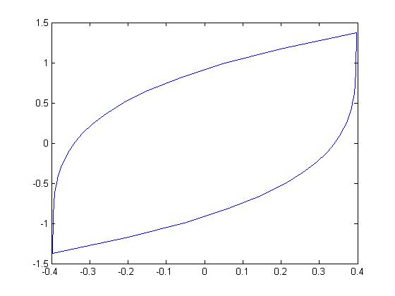
Fig. 1 shows the 2-dimensional ellipsoids generated by the matrix as follows
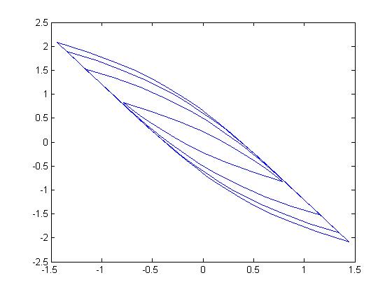
In the next discussion, the systems are assumed always as a controllable systems and the geometry is a -dimensional smooth zonotope.
2.3 The Definition of the Control Ability with time Attributy
As we know, the bigger of the controllability region is, the more the controllable states in the state space are, and but whether the control ability of the dynamical systems is stronger or not. In the next subsection, it will proven that for the control/reach problems, the bigger of the controllability region, the bigger the solution space of the input variables is, and then the better the some closed-loop control performance is. Thus, the size and shape of the controllability region is used to define and describe the control ability with time attribute.
Next, 2 equivalent definitions on the stronger control ability between the two differential controlled plants, or of one controlled plants with two sets of systems parameters are purposed as follows.
Definition 1
For the given controllability regions and of the two LCT Systems and , if the given and , the control ability of the systems at state is stronger than the systems . If for any , the control ability of the systems at all state in is stronger than the systems , the control ability of the systems is stronger than the systems .
Definition 2
For any , if the two controllability regions and of the LCT Systems and satisfy
| (12) |
the control ability of the systems is stronger than the systems . if and for any satisfy
| (13) |
the control ability of the systems is not weaker than the systems .
According to the above definitions, the control ability of the dynamical systems can be compared for many control engineering problems as stated above.
3 Theorem on Relation between the Open-loop Control Ability and the Closed-loop Performances
Before discussing on relation between the open-loop control ability and the closed-loop performances, a time-optimal property for the boundary of controllability region is stated as follows [9], [10].
Property 3
If the LCT Systems (1) is controllable and the given state satisfy
| (14) |
the time waste of the time-optimal control problem for stabilizing the initial state to the original of the state space (or for controlling the state at the original to the expecting state ) under the input amplitude constraint is , that is, the fewest control time is .
Based on the definition of the control ability and above properties, a theorem on the relations among the open-loop control ability, the solution space of the input variables, and the closed-loop performances are purposed and proven as follows.
Theorem 1
It is assumed that two LCT Systems and are controllable, and their controllability regions are and respectively. If we have
| (15) |
for the control problem stabilizing the state to the original of the state space (or for controlling the state at the original to the expecting state ), the following conclusions hold under the input amplitude constraint .
1) The time waste of the time-optimal control for the system is not more than that of , that is, there exist some control strategies with the less control time and the faster response speed for the system .
2) There exist more control strategies for the system , that is, the bigger the controllability region is, the bigger the solution space of the input variable for the control problems, the easier designing and implementing the control are.
The above theorem will be proven by the discretization model with a sufficient small sampling period for approximating the LCT systems. The discretization model with a small sampling period for the LCT systems (1) should be as follows [12] [3]
| (16) |
where and are the state variable and input variable of the discretization model, respectively.
| (17) |
Therefore, when , the linear discrete-time (LDT) systems will approxiamte the LCT systems .
Proof of Theorem 1 Beacuse that the LCT systems can be approximated by the LDT systems with a sufficient small sampling-period , the conclussions of Theorem 1 in paper [21] for the LDT systems are still established when and then the conclussions in Theorem 1 for the LCT systems, similar to that Theorem 1 in paper [21], will be regarded as true. \qed
By Theorem 1, we have the following discussions:
(1) Not only the time waste can be reduced by promoting the control ability, but also other closed-loop performance related the control time waste can be improved.
(2) In fact, that the solution space of the input variable for the control problems is bigger implies that the control strategies in the solution space are with better robustness, and then the closed-loop control systems is also with better robustness.
(3) According to the theorem, the control ability defined and discussed here is indeed a control ability with time attributy. In fact, optimizing the control ability of the open-loop systems is to equal to promote some closed-loop performance indices related to the control time.
Therefore, optimizing the open-loop control ability with time attribute are with very greater signification and it’s very necessary to optimize the control ability for these practical control engineering problems. To optimize the control ability, it is necessary to establish the quantify analysis and computing method for that. An analytical computing equation for the volume of the controllability region for the LDT systems is deduced in paper [20] and the some analytical factors about the shape of the controllability region can be got by deconstructing the volume equation. Next, the similar studies for the LCT systems are carried out and then based on these analytical expressions of the volume and shape factors, the optimizing and promoting methods for the control ability can be set up conveniently.
4 The Volume Computing for the Smooth Zonotope for the Matrix with Different Eigenvalues
The volume computing problem for the zonotope generated by a matrix pair is discussed and two recurssive computing methods with the low time complexity are deduced in paper [20]. Furthermore, an analytic volume-computing theorem about the zonotope that the matrix is with different real eigenvalues are purposed and proven. In paper [19], the analytic volume-computing theorem for that the matrix is with real repeated eigenvalues is proven also. Because that the narrow controllability region and reachability region can be described by the zonotope generated by the matrix pair, these results on the recurrsive and analytic volume computing also are used to analyze these regions and control abilities for the LDT systems. Later, these computing and analyzing methods for the LDT systems in papers [20] [19] wlii be generalized to the LCT systems.
4.1 the recurrsive computing of the volume of the smooth zonotope
As the proof of Theorem 1, the LCT systems can be approximated by a LDT systems with a sufficient small sampling-period , and then the volume computing problem for the controllability region of the LCT systems can be transformated as that for LDT systems in papers [20] [19].
It is assumed the sufficient small sampling-period is , the controllability region defined in Eq. (8) can be represented approximately as follows
| (18) |
or
| (19) |
where is the integer part of . Therefore, according to the above approximation equations, the controllability region can be regarded as a zonotope generated by the matrix pair as Eq. (17), and then the recurssive volume-computing methods for the controllability regions fo the LDT systems in Section 2 and Section 3 of paper [20] can be applied to that of the LDT systems.
4.2 the analytical computing of the volume of the time-infinite smooth zonotope
In paper [20], an analytic volume-computing equation for the zonotope generated by the matrix pair with different real eigenvalues of matrix is proven. In fact, the region defined by Eq. (19) is a special zonotope defined in paper [20]. Therefore, the quantifying and maximizing of the controllability region can be carried out based on the results in paper [20]. The results in the volume computation of the zonotope generated by the matrix pair , in Theorem 2 and Theorem 3 of paper [20] can be summarized and generalized to the LCT systems. Hence, we have the following theorem about the analytical volume computing for the infinite-time controllability region of the LCT systems.
Theorem 2
If matrix is with different eigenvalues in the interval and , the volume of the infinite-time smooth zonotope generated by matrix pair can be computed analytically by the following equation:
| (20) |
where and are the -th eigenvalue and the corresponding unit left eigenvector of matrix , matrix is the matrix transforming the matrix as a diagonal matrix.
Proof of Theorem 2 Similar to above approximation method by the sampling model, the smooth zonotope generated by the matrix pair can be approximated by the zonotope generated by the matrix pair as Eq. (17). When the matrix is with different eigenvalues in interval , the matrix is also with different eigenvalues in interval . And then, by the Theorem 2 in paper [20], we have the following volume computation of the zonotope generated by as follows.
| (21) |
So, when , we have
| (22) |
that is, the theorem is true. \qed
Based on the above theorem, the volume of the controllability region when can be computed analytically. Furthermore, some analytical factors describing the shape of the can be got by deconstructing the analytical volume computing equation (20). These analytical expressions for these volume and shape factors can be describe quantitatively the control ability of the dynamical systems, and then optimizing these volume and shape factors is indeed maximizing the control ability.
4.3 Decoding the Controllability Region
According to the volume computing equation (20), some factors described the shape and size of the controllability region, that is, the control ability of the dynamical systems, are deconstructed as follows.
| (23) | ||||
| (24) | ||||
| (25) |
The above analytical factors can be called respectively as the shape factor, the side length of the circumscribed rhombohedral, and the modal controllability. In fact, the shape factor is also the eigenvalue evenness factor of the linear system, and can describe the control ability caused by the eigenvalue distribution. In addition, the modal controllability factor have been put forth by papers [2] [7] [5] [4], and will not be discussed here.
4.3.1 The Shape Factor of the Reachability Region and the Eigenvalue Evenness Factor of the Linear System
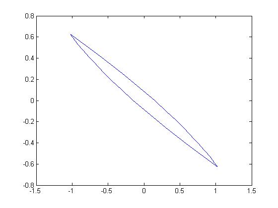
Fig. 2 shows the 2-dimensional smooth zonotopes , i.e., the terminal time , generated by the 3 matrix pairs that the matrix is with the different eigenvalues and matrix is a same vector, and Fig. 3 shows the 2-dimensional smooth zonotopes generated by the diagonal matrix pairs of these 3 matrix pairs , that is, the smooth zonotopes in Fig. 3 are in the invariant eigen-space.
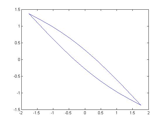
(a) (-2.9,-0.75,0.5891)
(b) (-2.9,-1.75,0.2473)
(c) (-2.9,-2.75,0.0265)
(a) (-2.9,-0.75,0.5891)
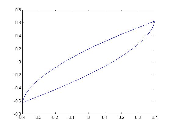
(b) (-2.9,-1.75,0.2473)
(c) (-2.9,-2.75,0.0265)
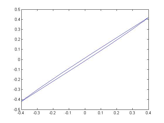
From these figures, we can see, when the two eigenvalues of the matrix are approximately equal, the minimum distances of the boundary of the region to the original will be approximately zero, and the region will be flattened. Similar casees are also for the -dimensional smooth zonotope generated by the matrix pair. Therefore, the distributions of all eigenvalues of the matrix are even, the ratio between the minimum and maximum distance of the boundary of the smooth zonotope generated by the pair can be avoided as a small value and the smooth zonotope will be avoided flattened.
The factor deconstructed from the volume computing equation (20) can be used to describe the uniformity of the biggest distances of the region in eigenvectors. The bigger the value of the factor , the bigger the ratio between the minimum and maximum distances of the bounded of the region is, and then the greater the volume of the region is.
Otherwise, the factor can be used to describe the evenness of the eigenvalue distribution of the linear system . The bigger the value of the factor , the bigger the controllable region of the system is, and the stronger the control ability of the systems is.
4.3.2 The circumscribed hypercube and circumscribed rhombohedral of the controllability region
The factor is indeed the biggest distance of the region in the -dimensional coordinate of the eigen-space (shown as in Fig. 3 ), that is, the side lengths of the circumscribed hypercube of the region are . By the volume equation (20), the volume of the region can be represented as the production of the volume of the circumscribed hypercube and the shape factor
Because that these expressions of the volume and the shape factors can describe accurately the size and shape of the smooth zonotope generated by the matrix pair, i.e., the control ability of the dynamical systems [21], these expressions can be used conveniently to be the objective function or the constrained conditions for the optimizing problems of the control ability of dynamical systems.
5 The Control Ability for the Systems with the Repeated real Eigenvalues
5.1 A Property about the Control Ability for the Systems with the Repeated Eigenvalues
In the last section, the volume of the smooth zonotope generated by the matrix pair , correspondingly the control ability of the linear systems, is discussed for the matrix with different real eigenvalues. Next, the volume is discussed for that the matrix is with the repeated real eigenvalues.
When some eigenvalues of matrix are the repeated eigenvalues, the matrix can be transformed as a Jordan matrix by a similar transformation in the matrix theory. In view of this, the following discussion are only carried out for the Jordan matrix. For the volume of the smooth zonotope generated by the Jordan matrix pair , a following theorem about the relation between the volume and matrix can be stated and proven firstly.
Theorem 3
The volume of the smooth zonotope generated by the Jordan matrix pair has relation only to the last rows of the matrix blocks of the matrix , corresponding to the each Jordan block of the matrix , and has no relation to other rows.
The conclusion in Theorem 3 is consistent with the conlusion, in control theory, that the state controllability of the systems has relation only to the last rows of these matrix blocks of the matrix , corresponding to the each Jordan block of the Jordan matrix , and has no relation to other rows. According to Theorem 3, for simplifying the volume computation for the Jordan matrix pair , the rows of matrix entirely unrelated to the volume will be regarded as 0.
Proof: Without loss of the generality, the theorem is proven only for the Jordan matrix with one Jordan block, and other cases can be proven similarly.
When the matrix is with only one Jordan block, the two matrices of the matrix pair can be written as follows
| (26) |
the corrsponding two matrices of the matrix pair of the sampling model as follows
| (27) |
And then, the matrix transformated the matrix as a Jordan matrix is as follows
| (28) |
where ’*’ means some value. Therefore, we have
| (29) |
and the corresponding matrices of the Jordan matrix pair are as follows
| (35) | ||||
| (41) |
Therefore, by Theorem 3 in paper [19], the volume of the zonotope generated by the Jordan matrix pair has relation only to the last rows of the matrix blocks of the matrix , corresponding to the each Jordan block of the matrix , and has no relation to other rows, that is, by Eq. (27), we can see, the approximating-zonotope volume is only related to parameter of the LCT systems and not to other . Thus, considered that the LDT systems will be equal to the LCT systems when , we know, the conclusion of Theorem 3 holds. \qed
According to the theorem, the volume computation of the smooth zonotope for the Jordan matrix pair can be equivalent to the volume computation for the Jordan matrix pair , where .
5.2 Volume Computing for the Infinite-time Smooth Zonotope When the Jordan Matrix with Multiple Jordan Blocks
If the matrix is a Jordan matrix with multiple Jordan blocks, the Jordan matrix pair can be denoted by
| (42) |
where is the Jordan block number, is a Jordan block with the eigenvalue , the matrix block is . And then, we have
Similar to Theorem 5 for the LDT Jordan models with multiple Jordan blocks in paper [19], a theorem about the volume computation of the infinite-time smooth zonotope for the LCT Jordan models with multiple Jordan blocks can be stated as follows.
Theorem 4
When all eigenvalues of the matrix satisfy , the volume of the infinite-time smooth zonotope generated by the Jordan matrix pair as Eq. (42) is computed as follows
| (43) |
When matrix isn’t a Jordan matrix, the volume of the infinite-time smooth zonotope generated by the matrix pair is computed as follows
| (44) |
where the matrix is the Jordan transformation matrix and the vector is the only unit left eigenvector of the matrix for the eigenvalue .
5.3 Decoding the Volume of the Controllability Region
According to the computing equation (44), some factors described the shape and size of the controllability religion, that is, the smooth zonotope generated by the matrix pair with the repeated eigenvalues, are deconstructed as follows.
| (45) | ||||
| (48) | ||||
| (49) |
where all are assumed as with the same sign. These 3 classes of factors are similar to the last section, called as the shape factor, the side length of the circumscribed rhombohedral, and the modal controllability. These factors can be describe the shape and size of the smooth zonotope, the control ability of the system, and the eigenvalue evenness factor of the linear system.
5.3.1 The Smooth Zonotope Shape Factor and the Eigenvalue Evenness Factor of the Linear System
Similar to the analysis for the matrix with different eigenvalues in last section, by Eq. (44), we can see, when some two eigenvalues of the two Jordan blocks of the system matrix are approximately equal, the minimum distance of the boundary of the smooth zonotope to the original of the stat space will be approximately zero, and the smooth zonotope will be flattened. Therefore, the distributions of all eigenvalues of the matrix are even, the ratio between the minimum and maximum distance of the boundary to original can be avoided as a small value and the smooth zonotope, that is, the control region, will be avoided flattened. And then, the volume of the smooth zonotope and the control ability will maintain a certain size.
The factor deconstructed from the volume computing equation (44) can be used to describe the uniformity the distance of the boundary to the original in the eigenvector. The bigger the value of the factor , the bigger the ratio between the minimum and maximum distance of the boundary is, and then the greater the volume of the smooth zonotope.
Otherwise, the factor can be used to describe the evenness of the eigenvalue distribution of the linear system . The bigger the value of the factor , the bigger the controllable region of the system is, and the stronger the control ability of the systems is.
5.3.2 The circumscribed hypercube and circumscribed rhombohedral of the controllability region
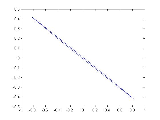
Fig. 4 shows the 2-dimensional smooth zonotopes by the 3 Jordan matrix pairs as follows
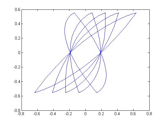
By Fig. 4, we know, the factor is indeed the biggest distance of the boundary of the smooth zonotope in the each eigenvector, that is, the side lengths of the circumscribed hypercube of the smooth zonotope in the invariant eigen-space are . By the volume equation (44), the volume of the smooth zonotope region can be represented as the production of the volume of the circumscribed hypercube and the shape factor
By Theorem, 3, we know, the volume of the smooth zonotope generated by the Jordan matrix pair has relation only to the last rows of the matrix blocks of the matrix , corresponding to the each Jordan block of the matrix , and has no relation to other rows. But from Fig. 4, we know, these ’other’ rows of matrix of Jordan matrix pair don’t affect the size of the volume but maybe affect the shape of the corresponding smooth zonotopes.
6 Numerical Experiments (It’s not available for now)
7 Conclusions
In this paper, the control ability with time attributy for the linear conti- nuous-time (LCT) systems are defined and analyzed by the volume computing for the controllability region. Firstly, a relation theorem about the open-loop control ability, the control strategy space (i.e., the solution space of the input variable for control problems), and the some closed-loop performance for the LCT systems is purposed and proven. This theorem shows us the necessity to optimize the control ability for the practical engineering problems. Secondly, recurssive volume-computing algorithms with the low computing complexities for the finite-time controllability region are discussed. Finally, two analytical volume computations of the infinite-time controllability region for the systems with different and repeated real eigenvalues are deduced, and then by deconstructing the volume computing equations, 3 classes of the shape factors are constructed. These analytical volume and shape factors can describe accurately the size and shape of the controllability region. Because the time-attribute control ability for LCT systems is directly related to the controllability region with the unit input variables (i.e. the input variable is with bounded value as 1), based on these analytical expressions on the volume and shape factors, the time-attribute control ability can be computed and optimized conveniently. And then, a noval researching field about the optimizing open-loop control ability and promoting the closed-loop control performance and robustness is expected to be founded in control theory and engineering.
References
- Bernstein and Michel [1995] D. Bernstein, A. Michel, A chronological bibliography on saturating actuators, Inter. J. of Robust and Nonlinear Control 5 (1995) 375–380.
- Chan [1984] S. Chan, Modal controllability and observability of power-system models, International Journal of Electrical Power & Energy Systems 6 (1984) 83–88.
- Chen [1998] C.T. Chen, Linear system theory and design, Oxford University Press, Inc. New York, NY, USA, 3rd edition, 1998.
- Chen et al. [2001] Y. Chen, S. Chen, Z. Liu, Quantitative measures of modal controllability and observability in vibration control of defective and near-defective systems, Journal of Sound and Vibration 248 (2001) 413–26.
- Choi et al. [2000] J.W. Choi, U.S. Park, S.B. Lee, Measures of modal controllability and observability in balanced coordinates for optimal placement of sensors and actuators: a flexible structure application, in: Proceedings of the SPIE, volume 3984, pp. 425–436.
- Georges [1995] D. Georges, The use of observability and controllability gramians or functions for optimal sensor and actuator location in finite-dimensional systems, in: Proc. of IEEE Conf. on Decision and Control, New Orleans, LA, USA, p. 3319–3324.
- Hamdan and Eladbdalla [1988] A. Hamdan, A. Eladbdalla, Geometric measures of modal controllability and observability of power system models, Electric Power Systems Research 15 (1988) 147–155.
- Hamdan and Jaradat [2014] A.M.A. Hamdan, A.M. Jaradat, Modal controllability and observability of linear models of power systems revisited, Arabian Journal for Science and Engineering 39 (2014) 1061–1066.
- Hu and Lin [2001] T. Hu, Z. Lin, Control systems with actuator saturation: analysis and design, BirkhTauser, Boston, 2001.
- Hu et al. [2002] T. Hu, Z. Lin, L. Qiu., An explicit description of the null controllable regions of linear systems with saturating actuators, Systems & Control Letters 47 (2002) 65–78.
- Ilkturk [2015] U. Ilkturk, Observability Methods in Sensor Scheduling, Ph.D. thesis, ARIZONA STATE UNIVERSITY, 2015.
- Kailath [1980] T. Kailath, Linear systems, Prentice-Hall, Englewood Cliffs, NJ, 1980.
- Kalman et al. [1963] R.E. Kalman, Y.C. Ho, K.S. Narendra, Controllability of dynamical systems, Contributions to Differential Equations 1 (1963) 189–213.
- Longman et al. [1982] R.W. Longman, T.L. S. W. Sirlin, G. Sevaston, Optimization of actuator placement via degree of controllability criteria including spillover considerations, AIAA/AAS Astrodynamics Conference, San Diego, California, Paper No. AIAA-82-1434 (1982).
- Pasqualetti et al. [2014] F. Pasqualetti, S. Zampieri, F. Bullo, Controllability metrics, limitations and algorithms for complex networks, IEEE Trans. on Control of Network Systems 1 (2014) 40–52.
- VanderVelde and Carignan [1982] W. VanderVelde, C. Carignan, A dynamic measure of controllability and observability for the placement of actuators and sensors on large space structures, Technical Report, NASA-CR-168520, SSL-2-82, 1982.
- Viswanathan et al. [1984] C.N. Viswanathan, R.W. Longman, P.W. Likins, A degree of controllability definition - fundamental concepts and application to modal systems, J. Guidance, Control, Dynamics 7 (1984) 222–230.
- Zhao [2020a] M.W. Zhao, Analytical expression and deconstruction of the volume of the controllability ellipsoid, arXiv:2004.05528 (2020a) 10.
- Zhao [2020b] M.W. Zhao, Analytical factors for describing the control ability of linear discrete-time systems, arXiv:2004.07982 (2020b).
- Zhao [2020c] M.W. Zhao, Exact volume of zonotopes generated by a matrix pair, arXiv:2004.05530 (2020c) 20.
- Zhao [2020d] M.W. Zhao, Relations among open-loop control ability, control strategy space and closed-loop performance for linear discrte-time systems, arXiv:2004.05619 (2020d) 13.