Contrast-independent partially explicit time discretizations for nonlinear multiscale problems

Eric T. Chung ¹¹1Department of Mathematics, The Chinese University of Hong Kong (CUHK), Hong Kong SAR, Yalchin Efendiev²²2Department of Mathematics, Texas A&M University, College Station, TX 77843, USA & North-Eastern Federal University, Yakutsk, Russia, Wing Tat Leung³³3Department of Mathematics, University of California, Irvine, USA, Wenyuan Li⁴⁴4Department of Mathematics, Texas A&M University, College Station, TX 77843, USA

Abstract

This work continues a line of works on developing partially explicit methods for multiscale problems. In our previous works, we have considered linear multiscale problems, where the spatial heterogeneities are at subgrid level and are not resolved. In these works, we have introduced contrast-independent partially explicit time discretizations for linear equations. The contrast-independent partially explicit time discretization divides the spatial space into two components: contrast dependent (fast) and contrast independent (slow) spaces defined via multiscale space decomposition. Following this decomposition, temporal splitting is proposed that treats fast components implicitly and slow components explicitly. The space decomposition and temporal splitting are chosen such that it guarantees a stability and formulate a condition for the time stepping. This condition is formulated as a condition on slow spaces. In this paper, we extend this approach to nonlinear problems. We propose a splitting approach and derive a condition that guarantees stability. This condition requires some type of contrast-independent spaces for slow components of the solution. We present numerical results and show that the proposed methods provide results similar to implicit methods with the time step that is independent of the contrast.

1 Introduction

Nonlinear problems arise in many applications and they are typically described by some nonlinear partial differential equations. In many applications, these problems have multiscale nature and contain multiple scales and high contrast. Examples include nonlinear porous media flows (e.g., Richards’ equations, Forchheimer flow, and so on, e.g., [21, 4]), where the media properties contain many spatial scales and high contrast. Because of high contrast in the media properties, these processes also occur on multiple times scales. E.g., for nonlinear diffusion, the flow can be fast in high conductivity regions, while the flow is slow in low conductivity regions. Because of disparity of time scales, special temporal discretizations are often sought, which is the main goal of the paper in the context of multiscale problems.

When the media properties are high, the flow and transport become fast and requires small time step to resolve the dynamics. Implicit discretization can be used to handle fast dynamics; however, this requires solving large-scale nonlinear systems. For nonlinear problems, explicit methods are used when possible to avoid solving nonlinear systems. The main drawback of explicit methods is that they require small time steps that scale as the fine mesh and depend on physical parameters, e.g., the contrast. To alleviate this issue, we propose a novel nonlinear splitting algorithm following our earlier works [23, 24] for linear equations. The main idea of our approaches is to use multiscale methods on a coarse spatial grid such that the time step scales as the coarse mesh size.

Next, we give a brief overview of multiscale methods for spatial discretizations that are used in our paper. Multiscale spatial algorithms have been extensively studied for linear and nonlinear problems. For linear problems, many multiscale methods have been developed. These include homogenization-based approaches [18, 34], multiscale finite element methods [18, 27, 33], generalized multiscale finite element methods (GMsFEM) [6, 7, 8, 11, 16], constraint energy minimizing GMsFEM (CEM-GMsFEM) [9, 10], nonlocal multi-continua (NLMC) approaches [12], metric-based upscaling [38], heterogeneous multiscale method [15], localized orthogonal decomposition (LOD) [26], equation-free approaches [39, 41], multiscale stochastic approaches [29, 30, 28], and hierarchical multiscale method [5]. For high-contrast problems, approaches such as GMsFEM and NLMC are developed. For example, in the GMsFEM [9], multiple basis functions or continua are designed to capture the multiscale features due to high contrast [10, 12]. These approaches require a careful design of multiscale dominant modes. For nonlinear problems, linear multiscale basis functions can be replaced by nonlinear maps [19, 20, 17].

Our proposed approaches follow concepts developed in [23, 24] for linear equations. In these works, we design splitting algorithms for solving flow and wave equations. In both cases, the solution space is divided into two parts, coarse-grid part, and the correction part. Coarse-grid solution is computed using multiscale basis functions with CEM-GMsFEM. The correction part uses special spaces in the complement space (complement to the coarse space). A careful choice of these spaces guarantees that the method is stable. Our analysis in [23, 24] shows that for the stability, the correction space should be free of contrast and thus, this requires a special multiscale space construction. These splitting algorithms take their origin from earlier works [36, 43]. In this paper, we extend the linear concepts to nonlinear problems.

Splitting algorithms for nonlinear problems have often been used in the literature. Earlier approaches include implicit-explicit approaches and other techniques [3, 35, 1, 22, 2, 37, 42, 14, 25, 32, 40, 31, 13]. In many approaches, nonlinear contributions are roughly divided into two parts depending on whether it is easy to implicitly solve discretized system. For easy to solve part, implicit discretization is used, while for the rest, explicit discretization is used. However, in general, one can not separate these parts for the problems under the consideration. Our goal is to use splitting concepts and treat implicitly and explicitly some parts of the solution. As a result, we can use larger time steps that scale as the coarse mesh size.

Our approach starts a nonlinear dynamical system

u_{t}+f(u)+g(u)=0,

where $f(u)$ represents diffusion-like operator, while $g(u)$ represents reaction-like terms. In linear problems, for the stability, we formulate a condition that involves the time step, the energy and $L^{2}$ norm of the solution in complement space. This is a constraint for the time step. With an appropriate choice of the complement space, this condition guarantees the stability for the time steps that scale as the coarse mesh size. To obtain similar conditions for nonlinear problems, we carry out the analysis for nonlinear $f(u)$ and $g(u)$ functions. The analysis reveals conditions that are required for stability. The conditions of multiscale spaces turn out to share some similarities to those for nonlinear multiscale methods [17]. We remark several observations.

•

Additional degrees of freedom are needed for dynamic problems, in general, to handle missing information.
•

We note that restrictive time step scales as the coarse mesh size and, thus, much coarser.

We present several numerical results. In our numerical results, we consider two cases. In the first case, we take the reaction term, $g(u)$ , to be nonlinear, while the diffusion term, $f(u)$ , to be linear. In the second case, we consider both to be nonlinear and use for $f(u)$ the form $f(u)=-div(\kappa(x,u)\nabla u)$ . The media properties for the diffusion is taken to be heterogeneous and we choose smooth and singular source terms. We compare the proposed approach to the approach, where all degrees of freedom are handled implicitly. We show that the proposed methods provide an approximation similar to fully implicit methods.

The paper is organized as follows. In the next section, we provide some preliminaries. In Section 3, we present our main assumptions and stability estimates for fine-grid problem. In Section 4, we describe the partially explicit method and its stability, following some discussions in Section 5. Numerical results are presented in Section 6.

2 Problem Setting

We consider the following equation

\displaystyle u_{t}=-f(u)-g(u),

(2.1)

where $f=\cfrac{\delta F}{\delta u}$ and $g=\cfrac{\delta G}{\delta u}$ which are the variational derivative of energies $F(u):=\int_{\Omega}E_{1}(u)$ and $G(u):=\int_{\Omega}E_{2}(u)$ . Here, $f$ is assumed to be contrast dependent nonlinear (or linear) (i.e., $f$ introduces stiffness in the system) while $g$ is contrast independent (i.e., $g$ does not introduce stiffness).

We assume $f(u)\in V^{*}$ and $g(u)\in L^{2}(\Omega)$ for all $u\in V$ . We can then consider the weak formulation of the problem, namely, finding $u\in V$ such that

(u_{t},v)=-(f(u),v)_{V^{*},V}\;\forall v\in V.

To simplify the notation, we will simply write $(\cdot,\cdot)$ instead of $(\cdot,\cdot)_{V^{*},V}$ in the following discussion.

Example 1: For $F(u)=\cfrac{1}{2}\int_{\Omega}\kappa|\nabla u|^{2}$ and $G(u)=0$ , we will have $f(u^{\prime})=\cfrac{\delta F}{\delta u}\in H^{1}(\Omega)=(H^{1}(\Omega))^{*}$ for $V=H^{1}(\Omega)$ .

(\cfrac{\delta F}{\delta u}(u^{\prime}),v)=\int_{\Omega}\kappa\nabla u^{\prime}\cdot\nabla v,

and thus, we have

-f(u^{\prime})=\nabla\cdot(\kappa\nabla u^{\prime}).

In strong form, we have

u_{t}=\nabla\cdot(\kappa\nabla u).

Example 2: For $F=\cfrac{1}{p}\int\kappa|\nabla u|^{p}$ and $G(u)=0$ , we will have $f(u^{\prime})=\cfrac{\delta F}{\delta u}\in W^{1,\frac{p}{p-1}}(\Omega)=(W^{1,p}(\Omega))^{*}$ for $V=W^{1,p}(\Omega)$

(\cfrac{\delta F}{\delta u}(u^{\prime}),v)=\int\kappa|\nabla u^{\prime}|^{p-2}\nabla u^{\prime}\cdot\nabla v,

and thus, we have

-f(u^{\prime})=\nabla\cdot(\kappa|\nabla u^{\prime}|^{p-2}\nabla u^{\prime}).

In strong form, we have

u_{t}=\nabla\cdot(\kappa|\nabla u|^{p-2}\nabla u).

In the following discussion, we will make the following assumptions on the second variational derivative of $F$ and $G$ .

•

The second variational derivative $\delta^{2}F$ and $\delta^{2}G$ satisfy

$\delta^{2}F(u)(v,v)\geq c(u)\|v\|_{V}^{2}\;\forall u,v\in V$

$\delta^{2}G(u)(v,v)\geq b(u)\|v\|^{2}\;\forall u,v\in V,$

where $0\leq c(u)<\infty$ and $-\underline{b}\leq b(u)<\infty$ are independent on $v$ .
•

The second variational derivative $\delta^{2}F$ and $\delta^{2}G$ are bounded. That is,

$|\delta^{2}F(u)(w,v)|\leq C(u)\|v\|_{V}\|w\|_{V}\;\forall u,v,w\in V$

$|\delta^{2}G(u)(w,v)|\leq B\|v\|_{L_{2}}\|w\|_{L_{2}}\;\forall u,v,w\in V,$

where $0<C(u)<\infty$ and $0<B<\infty$ are independent on $v,w$ .

3 Discretization

To solve the problem, a standard method is finite element approach. We can consider the numerical solution $u_{H}(t,\cdot)\in V_{H}$ satisfies

\displaystyle(u_{H,t},v)=-(f(u)+g(u),v)\;\forall v\in V_{H},

(3.1)

where $V_{H}$ is a finite element space in $V$ .

For the time discretization, we can consider two simplest discretizations which are forward Euler and backward Euler methods. For the forward Euler method, we consider $\{u_{H}^{k}\}_{k=0}^{N}\subset V_{H}$ such that

(\cfrac{u_{H}^{n+1}-u_{H}^{n}}{\Delta t},v)+(f(u_{H}^{n})+g(u_{H}^{n}),v)=0\;\forall v\in V_{H}.

For the backward Euler method, we consider $\{u_{H}^{k}\}_{k=0}^{N}\subset V_{H}$ such that

(\cfrac{u_{H}^{n+1}-u_{H}^{n}}{\Delta t},v)+(f(u_{H}^{n+1})+g(u_{H}^{n+1}),v)=0\;\forall v\in V_{H}.

Next, we would like to derive stability conditions for backward and forward Euler methods.

Since

F(u_{H}^{n})=F(u_{H}^{n+1})-(f(u_{H}^{n+1}),u_{H}^{n+1}-u_{H}^{n})+\cfrac{1}{2}\delta^{2}F(\xi_{1}^{n})(u_{H}^{n+1}-u_{H}^{n},u_{H}^{n+1}-u_{H}^{n})

and

G(u_{H}^{n})=G(u_{H}^{n+1})-(g(u_{H}^{n+1}),u_{H}^{n+1}-u_{H}^{n})+\cfrac{1}{2}\delta^{2}G(\xi_{2}^{n})(u_{H}^{n+1}-u_{H}^{n},u_{H}^{n+1}-u_{H}^{n})

for some $\xi_{i}^{n}=(1-\lambda_{i})u_{H}^{n+1}+\lambda_{i}u_{H}^{n}$ with $\lambda_{i}\in(0,1)$ and $i=1,2$ , we have

	$\displaystyle 0=$	$\displaystyle(\cfrac{u_{H}^{n+1}-u_{H}^{n}}{\Delta t},u_{H}^{n+1}-u_{H}^{n})+(f(u_{H}^{n+1})+g(u_{H}^{n+1}),u_{H}^{n+1}-u_{H}^{n})$
	$\displaystyle=$	$\displaystyle\cfrac{1}{\Delta t}\\|u_{H}^{n+1}-u_{H}^{n}\\|^{2}+F(u_{H}^{n+1})-F(u_{H}^{n})+G(u_{H}^{n+1})-G(u_{H}^{n})$
		$\displaystyle+\cfrac{1}{2}\delta^{2}F(\xi_{1}^{n})(u_{H}^{n+1}-u_{H}^{n},u_{H}^{n+1}-u_{H}^{n})+\cfrac{1}{2}\delta^{2}G(\xi_{2}^{n})(u_{H}^{n+1}-u_{H}^{n},u_{H}^{n+1}-u_{H}^{n})$
	$\displaystyle\geq$	$\displaystyle\Big{(}\cfrac{1}{\Delta t}+b(u)\Big{)}\\|u_{H}^{n+1}-u_{H}^{n}\\|^{2}+F(u_{H}^{n+1})-F(u_{H}^{n})+G(u_{H}^{n+1})-G(u_{H}^{n})+\cfrac{c(u)}{2}\\|u_{H}^{n+1}-u_{H}^{n}\\|_{V}^{2}.$

We have

	$\displaystyle F(u_{H}^{n+1})+G(u_{H}^{n+1})$	$\displaystyle\leq F(u_{H}^{n+1})+G(u_{H}^{n+1})+\cfrac{c(u)}{2}\\|u_{H}^{n+1}-u_{H}^{n}\\|_{V}^{2}+\Big{(}\cfrac{1}{\Delta t}-\underline{b}\Big{)}\\|u_{H}^{n+1}-u_{H}^{n}\\|^{2}$
		$\displaystyle\leq F(u_{H}^{n})+G(u_{H}^{n})$

for any $\Delta t$ and thus, backward Euler method is stable if $\Delta t\underline{b}\leq 1$ .

Similarly, for forward Euler method, we can use

F(u_{H}^{n+1})=F(u_{H}^{n})+(f(u_{H}^{n}),u_{H}^{n+1}-u_{H}^{n})+\cfrac{1}{2}\delta^{2}F(\xi_{1}^{n})(u_{H}^{n+1}-u_{H}^{n},u_{H}^{n+1}-u_{H}^{n})

G(u_{H}^{n+1})=G(u_{H}^{n})+(g(u_{H}^{n}),u_{H}^{n+1}-u_{H}^{n})+\cfrac{1}{2}\delta^{2}G(\xi_{2}^{n})(u_{H}^{n+1}-u_{H}^{n},u_{H}^{n+1}-u_{H}^{n})

and obtain

	$\displaystyle 0=$	$\displaystyle(\cfrac{u_{H}^{n+1}-u_{H}^{n}}{\Delta t},u_{H}^{n+1}-u_{H}^{n})+(f(u^{n})+g(u_{H}^{n}),u_{H}^{n+1}-u_{H}^{n})$
	$\displaystyle=$	$\displaystyle\cfrac{1}{\Delta t}\\|u_{H}^{n+1}-u_{H}^{n}\\|^{2}+F(u_{H}^{n+1})-F(u_{H}^{n})+G(u_{H}^{n+1})-G(u_{H}^{n})$
		$\displaystyle-\cfrac{1}{2}\delta^{2}F(\xi_{1}^{n})(u_{H}^{n+1}-u_{H}^{n},u_{H}^{n+1}-u_{H}^{n})-\cfrac{1}{2}\delta^{2}G(\xi_{2}^{n})(u_{H}^{n+1}-u_{H}^{n},u_{H}^{n+1}-u_{H}^{n})$
	$\displaystyle\geq$	$\displaystyle(\cfrac{1}{\Delta t}-B)\\|u_{H}^{n+1}-u_{H}^{n}\\|^{2}+F(u_{H}^{n+1})-F(u_{H}^{n})+G(u_{H}^{n+1})-G(u_{H}^{n})-\cfrac{C(\xi^{n})}{2}\\|u_{H}^{n+1}-u_{H}^{n}\\|_{V}^{2}.$

Therefore, if $\Delta t\Big{(}\cfrac{C(\xi)}{2}\cfrac{\|u_{H}^{n+1}-u_{H}^{n}\|_{V}^{2}}{\|u_{H}^{n+1}-u_{H}^{n}\|^{2}}+B\Big{)}\leq 1$ for any $\xi=(1-\lambda)u_{H}^{k+1}+\lambda u_{H}^{k}$ with $0\leq k\leq N-1$ , we have

\displaystyle F(u_{H}^{n+1})+G(u_{H}^{n+1})

\displaystyle\leq F(u_{H}^{n})+G(u_{H}^{n}).

We can see that although forward Euler method is easier for implementation, we require a small time step for stability if $\sup_{v\in V_{H}}\cfrac{\|v\|_{V}^{2}}{\|v\|^{2}}$ or $C(\xi)$ is large.

We remark that in typical cases we will consider $\underline{b}$ and $B$ are not too large. Therefore, we have $\Delta t\underline{b}$ and $\Delta tB$ is small and the energy $G$ will not affect the stability too much.

4 Partially explicit scheme with space splitting

To obtain an efficient method, one can consider partially explicit scheme by splitting finite element space. We consider $V_{H}$ is a direct sum of two subspace $V_{H,1}$ and $V_{H,2}$ , namely, $V_{H}=V_{H,1}\oplus V_{H,2}$ . The finite element solution is then satisfying

	$\displaystyle(u_{H,1,t}+u_{H,2,t},v_{1})+(f(u_{H,1}+u_{H,2})+g(u_{H,1}+u_{H,2}),v_{1})$	$\displaystyle=0\;\forall v_{1}\in V_{H,1},$
	$\displaystyle(u_{H,1,t}+u_{H,2,t},v_{2})+(f(u_{H,1}+u_{H,2})+g(u_{H,1}+u_{H,2}),v_{2})$	$\displaystyle=0\;\forall v_{2}\in V_{H,2},$

where $u_{H}=u_{H,1}+u_{H,2}$ . We can use a partially explicit time discretization. For example, we can consider

	$\displaystyle(\cfrac{u_{H,1}^{n+1}-u_{H,1}^{n}}{\Delta t}+\cfrac{u_{H,2}^{n}-u_{H,2}^{n-1}}{\Delta t},v_{1})+(f(u_{H,1}^{n+1}+u_{H,2}^{n})+g(u_{H,1}^{n}+u_{H,2}^{n}),v_{1})$	$\displaystyle=0\;\forall v_{1}\in V_{H,1},$
	$\displaystyle(\cfrac{u_{H,1}^{n}-u_{H,1}^{n-1}}{\Delta t}+\cfrac{u_{H,2}^{n+1}-u_{H,2}^{n}}{\Delta t},v_{2})+(f(u_{H,1}^{n+1}+u_{H,2}^{n})+g(u_{H,1}^{n}+u_{H,2}^{n}),v_{2})$	$\displaystyle=0\;\forall v_{2}\in V_{H,2}.$

Energy stability

Lemma 4.1.

\begin{split}(f(u_{H}^{n+1})-f(u_{H,1}^{n+1}+u_{H,2}^{n}),u_{H}^{n+1}-u_{H}^{n})\leq\\ \cfrac{\bar{c}}{2}\|u_{H}^{n+1}-u_{H}^{n}\|_{V}^{2}+\Big{(}\cfrac{(1-\gamma)}{\Delta t}-(1+\gamma)\cfrac{B}{2}\Big{)}\sum_{i}\|u_{H,i}^{n+1}-u_{H,i}^{n}\|^{2},\end{split}

(4.1)

where $\bar{c}=\inf_{u\in V_{H}}c(u)$ and $\gamma=\sup_{v_{1}\in V_{H,1},v_{2}\in V_{H,2}}\cfrac{(v_{1},v_{2})}{\|v_{1}\|\|v_{2}\|}<1$ , we have

\cfrac{\gamma}{2\Delta t}\sum_{i}\|u_{H,i}^{n+1}-u_{H,i}^{n}\|^{2}+F(u_{H}^{n+1})+G(u_{H}^{n+1})\leq\cfrac{\gamma}{2\Delta t}\sum_{i}\|u_{H,i}^{n}-u_{H,i}^{n-1}\|^{2}+F(u_{H}^{n})+G(u_{H}^{n}).

Proof.

By substitute $v_{1}=u_{H,1}^{n+1}-u_{H,1}^{n}$ and $v_{2}=u_{H,2}^{n+1}-u_{H,2}^{n}$ , we have

	$\displaystyle\cfrac{1}{\Delta t}\\|u_{H,1}^{n+1}-u_{H,1}^{n}\\|^{2}+\cfrac{1}{\Delta t}(u_{H,2}^{n}-u_{H,2}^{n-1},u_{H,1}^{n+1}-u_{H,1}^{n})$
	$\displaystyle+(f(u_{H,1}^{n+1}+u_{H,2}^{n})+g(u_{H}^{n}),u_{H,1}^{n+1}-u_{H,1}^{n})$	$\displaystyle=0,$

and

	$\displaystyle\cfrac{1}{\Delta t}\\|u_{H,2}^{n+1}-u_{H,2}^{n}\\|^{2}+\cfrac{1}{\Delta t}(u_{H,1}^{n}-u_{H,1}^{n-1},u_{H,2}^{n+1}-u_{H,2}^{n})$
	$\displaystyle+(f(u_{H,1}^{n+1}+u_{H,2}^{n})+g(u_{H}^{n}),u_{H,2}^{n+1}-u_{H,2}^{n})$	$\displaystyle=0.$

Summing up the above two equations, we have

	$\displaystyle\cfrac{1}{\Delta t}\sum_{i}\\|u_{H,i}^{n+1}-u_{H,i}^{n}\\|^{2}+\cfrac{1}{\Delta t}\sum_{i\neq j}(u_{H,i}^{n}-u_{H,i}^{n-1},u_{H,j}^{n+1}-u_{H,j}^{n})$
	$\displaystyle+(f(u_{H,1}^{n+1}+u_{H,2}^{n})+g(u_{H}^{n}),u_{H}^{n+1}-u_{H}^{n})$	$\displaystyle=0.$

We first use

	$\displaystyle\cfrac{1}{\Delta t}\|\sum_{i\neq j}(u_{H,i}^{n}-u_{H,i}^{n-1},u_{H,j}^{n+1}-u_{H,j}^{n})\|$	$\displaystyle\leq\cfrac{\gamma}{\Delta t}\sum_{i\neq j}\\|u_{H,i}^{n}-u_{H,i}^{n-1}\\|\\|u_{H,j}^{n+1}-u_{H,j}^{n}\\|$
		$\displaystyle\leq\cfrac{\gamma}{2\Delta t}\sum_{i}\Big{(}\\|u_{H,i}^{n+1}-u_{H,i}^{n}\\|^{2}+\\|u_{H,i}^{n}-u_{H,i}^{n-1}\\|^{2}\Big{)}$

and obtain

		$\displaystyle\cfrac{1}{\Delta t}\sum_{i}\\|u_{H,i}^{n+1}-u_{H,i}^{n}\\|^{2}+\cfrac{1}{\Delta t}\sum_{i\neq j}(u_{H,i}^{n}-u_{H,i}^{n-1},u_{H,j}^{n+1}-u_{H,j}^{n})$
	$\displaystyle\geq$	$\displaystyle\cfrac{2-\gamma}{2\Delta t}\sum_{i}\\|u_{H,i}^{n+1}-u_{H,i}^{n}\\|^{2}-\cfrac{\gamma}{2\Delta t}\sum_{i}\\|u_{H,i}^{n}-u_{H,i}^{n-1}\\|^{2}.$

To prove the stability of the method, we can consider

F(u_{H}^{n})=F(u_{H}^{n+1})-(f(u_{H}^{n+1}),u_{H}^{n+1}-u_{H}^{n})+\cfrac{1}{2}\delta^{2}F(\xi_{1}^{n})(u_{H}^{n+1}-u_{H}^{n},u_{H}^{n+1}-u_{H}^{n})

G(u_{H}^{n+1})=G(u_{H}^{n})+(g(u_{H}^{n}),u_{H}^{n+1}-u_{H}^{n})+\cfrac{1}{2}\delta^{2}G(\xi_{2}^{n})(u_{H}^{n+1}-u_{H}^{n},u_{H}^{n+1}-u_{H}^{n})

for some $\xi_{i}^{n}=(1-\lambda_{i})u_{H}^{n+1}+\lambda_{i}u_{H}^{n}$ with $\lambda_{i}\in(0,1)$ and $i=1,2$ .

Therefore, we have

\begin{split}&(f(u_{H,1}^{n+1}+u_{H,2}^{n}),u_{H}^{n+1}-u_{H}^{n})\\ =&(f(u_{H,1}^{n+1}+u_{H,2}^{n})-f(u_{H}^{n+1}),u_{H}^{n+1}-u_{H}^{n})\\ &+F(u_{H}^{n+1})-F(u_{H}^{n})+\cfrac{1}{2}\delta^{2}F(\xi_{1}^{n})(u_{H}^{n+1}-u_{H}^{n},u_{H}^{n+1}-u_{H}^{n})\end{split}

(4.2)

and

		$\displaystyle(g(u_{H}^{n}),u_{H}^{n+1}-u_{H}^{n})$
	$\displaystyle=$	$\displaystyle G(u_{H}^{n+1})-G(u_{H}^{n})-\cfrac{1}{2}\delta^{2}G(\xi_{2}^{n})(u_{H}^{n+1}-u_{H}^{n},u_{H}^{n+1}-u_{H}^{n}).$

Thus, we obtain

		$\displaystyle\cfrac{\gamma}{2\Delta t}\sum_{i}\\|u_{H,i}^{n+1}-u_{H,i}^{n}\\|^{2}+\cfrac{(1-\gamma)}{\Delta t}\sum_{i}\\|u_{H,i}^{n+1}-u_{H,i}^{n}\\|^{2}+F(u_{H}^{n+1})+G(u_{H}^{n+1})+\cfrac{c(\xi^{n})}{2}\\|u_{H}^{n+1}-u_{H}^{n}\\|_{V}^{2}$
	$\displaystyle\leq$	$\displaystyle\cfrac{\gamma}{2\Delta t}\sum_{i}\\|u_{H,i}^{n}-u_{H,i}^{n-1}\\|^{2}+F(u_{H}^{n})+G(u_{H}^{n})+\cfrac{B}{2}\\|u_{H}^{n+1}-u_{H}^{n}\\|^{2}$
		$\displaystyle+(f(u_{H}^{n+1})-f(u_{H,1}^{n+1}+u_{H,2}^{n}),u_{H}^{n+1}-u_{H}^{n})$

and

\cfrac{B}{2}\|u_{H}^{n+1}-u_{H}^{n}\|^{2}\leq(1+\gamma)\cfrac{B}{2}\sum_{i}\|u_{H,i}^{n+1}-u_{H,i}^{n}\|^{2}.

(f(u_{H}^{n+1})-f(u_{H,1}^{n+1}+u_{H,2}^{n}),u_{H}^{n+1}-u_{H}^{n})\leq\cfrac{c(\xi^{n})}{2}\|u_{H}^{n+1}-u_{H}^{n}\|_{V}^{2}+\Big{(}\cfrac{(1-\gamma)}{\Delta t}-(1+\gamma)\cfrac{B}{2}\Big{)}\sum_{i}\|u_{H,i}^{n+1}-u_{H,i}^{n}\|^{2}

then we have

\cfrac{\gamma}{2\Delta t}\sum_{i}\|u_{H,i}^{n+1}-u_{H,i}^{n}\|^{2}+F(u_{H}^{n+1})+G(u_{H}^{n+1})\leq\cfrac{\gamma}{2\Delta t}\sum_{i}\|u_{H,i}^{n}-u_{H,i}^{n-1}\|^{2}+F(u_{H}^{n})+G(u_{H}^{n}).

∎

Lemma 4.2.

\displaystyle\cfrac{\bar{C}_{2}^{2}}{2\bar{c}}\sup_{v_{2}\in V_{H,2}}\cfrac{\|v_{2}\|_{V}^{2}}{\|v_{2}\|^{2}}+(1+\gamma)\cfrac{B}{2}\leq\cfrac{(1-\gamma)}{\Delta t},

(4.3)

where $\bar{c}=\inf_{u\in V_{H}}c(u)$ , $\bar{C}_{2}=\sup_{\xi\in V_{H}}C_{2}(\xi)$ and

C_{2}(\xi)=\sup_{v\in V_{H},w\in V_{H,2}}\cfrac{1}{\|v\|_{V}\|w\|_{V}}\delta^{2}F(\xi)(w,v)\leq C(\xi),

we have

\cfrac{\gamma}{2\Delta t}\sum_{i}\|u_{H,i}^{n+1}-u_{H,i}^{n}\|^{2}+F(u_{H}^{n+1})+G(u_{H}^{n+1})\leq\cfrac{\gamma}{2\Delta t}\sum_{i}\|u_{H,i}^{n}-u_{H,i}^{n-1}\|^{2}+F(u_{H}^{n})+G(u_{H}^{n}).

Proof.

For the proof of this lemma, we will show that if the condition of Lemma 4.2 holds, then the condition of Lemma 4.1 holds. For this reason, we will need to estimate $(f(u_{H}^{n+1})-(f(u_{H,1}^{n+1}+u_{H,2}^{n}),u_{H}^{n+1}-u_{H}^{n})$ . Similar to the proof in previous lemma, we consider

(f(u_{H}^{n+1}),u_{H}^{n+1}-u_{H}^{n})=(f(u_{H,1}^{n+1}+u_{H,2}^{n}),u_{H}^{n+1}-u_{H}^{n})+(\delta^{2}F(\tilde{\xi}^{n})(u_{H}^{n+1}-u_{H}^{n}),u_{H,2}^{n+1}-u_{H,2}^{n})

for some $\tilde{\xi}^{n}=(1-\tilde{\lambda})u_{H}^{n+1}+\tilde{\lambda}(u_{H,1}^{n+1}+u_{H,2}^{n})$ with $\tilde{\lambda}\in(0,1)$ . We have

	$\displaystyle(f(u_{H}^{n+1})-f(u_{H,1}^{n+1}+u_{H,2}^{n}),u_{H}^{n+1}-u_{H}^{n})$	$\displaystyle=(\delta^{2}F(\tilde{\xi}^{n})(u_{H}^{n+1}-u_{H}^{n}),u_{H,2}^{n+1}-u_{H,2}^{n})$
		$\displaystyle\leq C_{2}(\tilde{\xi}^{n})\\|u_{H}^{n+1}-u_{H}^{n}\\|_{V}\\|u_{H,2}^{n+1}-u_{H,2}^{n}\\|_{V}.$

Since

C_{2}(\tilde{\xi}^{n})\|u_{H}^{n+1}-u_{H}^{n}\|_{V}\|u_{H,2}^{n+1}-u_{H,2}^{n}\|_{V}\leq\cfrac{\bar{c}}{2}\|u_{H}^{n+1}-u_{H}^{n}\|_{V}^{2}+\cfrac{C_{2}^{2}(\tilde{\xi}^{n})}{2\bar{c}}\|u_{H,2}^{n+1}-u_{H,2}^{n}\|_{V}^{2},

we have

(f(u_{H}^{n+1})-f(u_{H,1}^{n+1}+u_{H,2}^{n}),u_{H}^{n+1}-u_{H}^{n})\leq\cfrac{\bar{c}}{2}\|u_{H}^{n+1}-u_{H}^{n}\|_{V}^{2}+\cfrac{C_{2}^{2}(\tilde{\xi}^{n})}{2\bar{c}}\|u_{H,2}^{n+1}-u_{H,2}^{n}\|_{V}^{2}.

\cfrac{\bar{C}_{2}^{2}}{2\bar{c}}\cfrac{\|u_{H,2}^{n+1}-u_{H,2}^{n}\|_{V}^{2}}{\|u_{H,2}^{n+1}-u_{H,2}^{n}\|^{2}}+(1+\gamma)\cfrac{B}{2}\leq\cfrac{(1-\gamma)}{\Delta t},

we have the condition formulated in Lemma 4.1

\begin{split}(f(u_{H}^{n+1})-f(u_{H,1}^{n+1}+u_{H,2}^{n}),u_{H}^{n+1}-u_{H}^{n})\leq\\ \cfrac{\bar{c}}{2}\|u_{H}^{n+1}-u_{H}^{n}\|_{V}^{2}+\Big{(}\cfrac{(1-\gamma)}{\Delta t}-(1+\gamma)\cfrac{B}{2}\Big{)}\sum_{i}\|u_{H,i}^{n+1}-u_{H,i}^{n}\|^{2}.\end{split}

(4.4)

By Lemma 4.1, we get the result. ∎

Example 1. For $F=\cfrac{1}{2}\int_{\Omega}\kappa|\nabla u|^{2}$ and $G(u)=0$ , we have

(\cfrac{\delta F}{\delta u},v)=\int_{\Omega}\kappa\nabla u\cdot\nabla v,

and

\delta^{2}F(u)(w,v)=\int_{\Omega}\kappa\nabla v\cdot\nabla w\;\forall u\in V,

and thus, we have

\bar{c}=C_{2}^{2}=1,\;B=0

and the partially explicit scheme is stable when

\cfrac{\Delta t}{2}\sup_{v_{2}\in V_{H,2}}\cfrac{\|\kappa^{\frac{1}{2}}\nabla v_{2}\|^{2}}{\|v_{2}\|^{2}}\leq(1-\gamma)\;\forall v_{2}\in V_{H,2}.

5 Discussions

5.1 $G=0$ case

First, we present some discussions for $G=0$ case. In this case, the first stability condition for partial explicit scheme is

\begin{split}(f(u_{H,1}^{n+1}+u_{H,2}^{n+1})-f(u_{H,1}^{n+1}+u_{H,2}^{n}),u_{H}^{n+1}-u_{H}^{n})\leq\\ \cfrac{\bar{c}}{2}\|u_{H}^{n+1}-u_{H}^{n}\|_{V}^{2}+\cfrac{(1-\gamma)}{\Delta t}\sum_{i}\|u_{H,i}^{n+1}-u_{H,i}^{n}\|^{2}.\end{split}

(5.1)

This condition can be understood as a nonlinear constraint on the “second space” that represents $u_{H,2}^{n}$ and in order to have a small bound, one needs to guarantee that $u_{H,1}^{n}$ captures important degrees of freeom. Indeed, the smallness of

{(f(u_{H,1}^{n+1}+u_{H,2}^{n+1})-f(u_{H,1}^{n+1}+u_{H,2}^{n}),u_{H}^{n+1}-u_{H}^{n})\over\|u_{H}^{n+1}-u_{H}^{n}\|_{V}^{2}}

is a condition on $u_{H,1}^{n}$ (on the coarse space) and requires that this term is chosen such that the difference is independent of the contrast. This condition is more evident in Lemma 4.2, where the condition on $V_{2}$ is

\cfrac{\bar{C}_{2}^{2}}{2\bar{c}}\sup_{v_{2}\in V_{H,2}}\cfrac{\|v_{2}\|_{V}^{2}}{\|v_{2}\|^{2}}\leq\cfrac{(1-\gamma)}{\Delta t}.

5.2 $G\not=0$ case.

In this case, we will first treat the nonlinear forcing explicitly and we will also discuss the case when $g(u)$ is partially explicit.

6 Numerical Results

In this section, we will present numerical results for various cases. We will consider several choices for $f(u)$ and $g(u)$ . For $f(u)$ , we will use diffusion operator for linear case

f(u)=-\nabla\cdot(\kappa\nabla u),

and nonlinear case

f(u)=-\nabla\cdot(\kappa\alpha(u)\nabla u).

(6.1)

In all examples, we will use two heterogeneous high contrast $\kappa(x)$ that represent the media, where one is more complex (more channels). As for $g(u)$ , we will consider several choices of nonlinear reaction terms as discussed below. This term will contain nonlinear reaction and steady state spatial source term. One source term will be more regular and the other more singular. The singular source term is chosen so that CEM solution requires additional basis functions as the source term contains subgrid features. In all numerical examples, the coarse mesh size is $\frac{1}{10}$ and the fine mesh size is $\frac{1}{100}$ . For the time discretization, we will consider the final time $T=0.05$ . In our numerical tests, we will compare three methods.

•

First, we will use implicit CEM to compute the solution without additional degrees of freedom (called “Implicit CEM” in our graphs).
•

Secondly, we will compute the solution with additional degrees of freedom using implicit CEM (called “Implicit CEM with additional basis” in our graphs).
•

Finally, we will compute the solution with additional degrees of fredoom using our proposed partially explicit approach (called “Partially Explicit Splitting CEM” in our graphs).

In all examples, we use Newton or Picard iterations to find the solution of nonlinear equations. In all examples, we observe that our proposed partially explicit method provides similar accuracy as the implicit CEM approach that uses additional degrees of freedom.

6.1 $V_{H,1}$ and $V_{H,2}$ constructions

In this section, we present a way to construct the spaces satisfying (4.3) based on linear problems. These spaces are constructed under the assumption that linear multiscale structure can be used to accurately model coarse-grid solution. It can be shown that the linear spaces satisfy (4.3) under some assumptions on $\kappa(x,u)$ (see (6.1)). Here, we follow our previous work [23]. As the constrained energy minimization basis functions are constructed such that they are almost orthogonal to a space $\tilde{V}$ , the CEM finite element space is a good option for $V_{H,1}$ . To find a $V_{H,2}$ satisfying the condition (4.3), we can use an eigenvalue problem to construct the local basis functions. We will first introduce the CEM finite element space, followed by the discussion of constructing $V_{H,2}$ . In the following, we let $V(S)=H_{0}^{1}(S)$ for a proper subset $S\subset\Omega$ .

6.1.1 CEM method

In this section, we introduce the CEM method for solving the problem (3.1). We will construct the finite element space by solving a constrained energy minimization problem. Let $\mathcal{T}_{H}$ be a coarse grid partition of $\Omega$ . For $K_{i}\in\mathcal{T}_{H}$ , we first need to define a set of auxiliary basis functions in $V(K_{i})$ . We solve

\displaystyle\int_{K_{i}}\kappa\nabla\psi_{j}^{(i)}\cdot\nabla v=\lambda_{j}^{(i)}s_{i}(\psi_{j}^{(i)},v)\;\forall v\in V(K_{i}),

where

\displaystyle s_{i}(u,v)=\int_{K_{i}}\tilde{\kappa}uv,\;\tilde{\kappa}=\kappa H^{-2}\;\text{or}\;\tilde{\kappa}=\kappa\sum_{i}\left|\nabla\chi_{i}\right|^{2}

with $\{\chi_{i}\}$ being a partition of unity functions corresponding to an overlapping partition of the domain. We then collect the first $L_{i}$ eigenfunctions corresponding to the first $L_{i}$ smallest eigenvalues. We define

V_{aux}^{(i)}:=\text{span}\{\psi_{j}^{(i)}:\;1\leq j\leq L_{i}\}.

We next define a projection operator $\Pi:L^{2}(\Omega)\mapsto V_{aux}\subset L^{2}(\Omega)$

s(\Pi u,v)=s(u,v)\;\forall v\in V_{aux}:=\sum_{i=1}^{N_{e}}V_{aux}^{(i)},

where $s(u,v):=\sum_{i=1}^{N_{e}}s_{i}(u|_{K_{i}},v|_{K_{i}})$ and $N_{e}$ is the number of coarse elements. We let $K_{i}^{+}$ be an oversampling domain of $K_{i}$ , which is a few coarse blocks larger than $K_{i}$ [9]. For each auxiliary basis functions $\psi_{j}^{(i)}$ , we can find a local basis function $\phi_{j}^{(i)}\in V(K_{i}^{+})$ such that

	$\displaystyle a(\phi_{j}^{(i)},v)+s(\mu_{j}^{(i)},v)$	$\displaystyle=0\;\forall v\in V(K_{i}^{+}),$
	$\displaystyle s(\phi_{j}^{(i)},\nu)$	$\displaystyle=s(\psi_{j}^{(i)},\nu)\;\forall\nu\in V_{aux}(K_{i}^{+})$

for some $\mu_{j}^{(i)}\in V_{aux}$ . We then define the space $V_{cem}$ as

\displaystyle V_{cem}

\displaystyle:=\text{span}\{\phi_{j}^{(i)}:\;1\leq i\leq N_{e},1\leq j\leq L_{i}\}.

The CEM solution $u_{cem}$ is given by

\displaystyle(\cfrac{\partial u_{cem}}{\partial t},v)+(f(u_{cem})+g(u_{cem}),v)=0\;\forall v\in V_{cem}.

Let $\tilde{V}:=\{v\in V:\;\Pi(v)=0\}$ and we can now construct $V_{H,2}$ .

6.1.2 Construction of $V_{H,2}$

The construction of $V_{H,2}$ is based on the CEM type finite element space. For each coarse element $K_{i}$ , we will solve an eigenvalue problem to get the second type of auxiliary basis. We obtain eigenpairs $(\xi_{j}^{(i)},\gamma_{j}^{(i)})\in(V(K_{i})\cap\tilde{V})\times\mathbb{R}$ by solving

\displaystyle\int_{K_{i}}\kappa\nabla\xi_{j}^{(i)}\cdot\nabla v

\displaystyle=\gamma_{j}^{(i)}\int_{K_{i}}\xi_{j}^{(i)}v,\;\ \forall v\in V(K_{i})\cap\tilde{V}

(6.2)

and rearranging the eigenvalues by $\gamma_{1}^{(i)}\leq\gamma_{2}^{(i)}\leq\cdots$ . For each $K_{i}$ , we choose the first few $J_{i}$ eigenfunctions corresponding to the smallest $J_{i}$ eigenvalues. We define $V_{aux,2}:=\text{span}\{\xi_{j}^{(i)}:1\leq i\leq N_{e},1\leq j\leq J_{i}\}$ . For each auxiliary basis function $\xi_{j}^{(i)}\in V_{aux,2}$ , we define a basis function $\zeta_{j}^{(i)}\in V(K_{i}^{+})$ such that $\mu_{j}^{(i),1}\in V_{aux,1}$ , $\mu_{j}^{(i),2}\in V_{aux,2}$ and

$\displaystyle a(\zeta_{j}^{(i)},v)+s(\mu_{j}^{(i),1},v)+(\mu_{j}^{(i),2},v)$	$\displaystyle=0,\;\forall v\in V(K_{i}^{+}),$	(6.3)
$\displaystyle s(\zeta_{j}^{(i)},\nu)$	$\displaystyle=0,\;\forall\nu\in V_{aux,1},$	(6.4)
$\displaystyle(\zeta_{j}^{(i)},\nu)$	$\displaystyle=(\xi_{j}^{(i)},\nu),\;\forall\nu\in V_{aux,2},$	(6.5)

where we use the notation $V_{aux,1}$ to denote the space $V_{aux}$ defined in Section 6.1.1. We define

V_{H,2}=\text{span}\{\zeta_{j}^{(i)}|\;1\leq i\leq N_{e},\;1\leq j\leq J_{i}\}.

6.2 Linear $f(u)$

In this subsection, we discuss the numerical results for

f(u)=-\nabla\cdot(\kappa\nabla u).

Equation $(\ref{eq1})$ becomes

\displaystyle u_{t}-\nabla\cdot(\kappa\nabla u)+g(u)=0.

(6.6)

For the time discretization, we consider the time step $\Delta t=\frac{T}{500}=10^{-4}$ .

Let $u_{h}$ be the fine mesh solution for Equation $(\ref{eq71})$ . We use Newton’s method to solve the following implicit equation.

(\frac{u^{n+1}_{h}-u^{n}_{h}}{\Delta t},v)+a(u^{n+1}_{h},v)+(g(u^{n+1}_{h}),v)=0\quad\forall v\in V_{h},

where $a(u^{n+1}_{h},v)=\int_{\Omega}\kappa\nabla u^{n+1}_{h}\cdot\nabla v$ and $(\cdot,\cdot)$ is the $L^{2}$ inner product. In finite element methods, let $\{\varphi_{i}\}_{i}$ be fine mesh basis functions. Let $m$ be the step number in Newton’s method. We have $u^{n+1,m+1}_{h}=\sum\limits_{i}U^{n+1,m+1}_{h,i}\varphi_{i}$ , $u^{n+1,m}_{h}=\sum\limits_{i}U^{n+1,m}_{h,i}\varphi_{i}$ and $u^{n}_{h}=\sum\limits_{i}U^{n}_{h,i}\varphi_{i}$ . Le $M$ and $A$ be the mass and stiffness matrices, respectively. Let $U^{n+1,m+1}_{h}=(U^{n+1,m+1}_{h,i})$ , $U^{n+1,m}_{h}=(U^{n+1,m}_{h,i})$ and $U^{n}_{h}=(U^{n}_{h,i})$ . We define

\displaystyle P(U^{n+1,m}_{h})=MU^{n+1,m}_{h}+\Delta t\cdot AU^{n+1,m}_{h}+\Delta t\cdot\mathcal{G}-MU^{n}_{h},

where $\mathcal{G}=(\mathcal{G}_{i})$

\mathcal{G}_{i}=(g(u^{n+1,m}_{h}),\varphi_{i}).

Then

\displaystyle(JP)(U^{n+1,m}_{h})=M+\Delta t\cdot A+\Delta t\cdot(J\mathcal{G}),

where $J\mathcal{G}=((J\mathcal{G})_{ij})$

(J\mathcal{G})_{ij}=\frac{\partial(g(u^{n+1,m}_{h}),\varphi_{i})}{\partial U^{n+1,m}_{h,j}}.

Then we have

U^{n+1,m+1}_{h}=U^{n+1,m}_{h}-(JP)^{-1}(U^{n+1,m}_{h})P(U^{n+1,m}_{h}).

Newton’s method for coarse mesh is similar. The partially explicit scheme is:

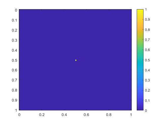
	$\displaystyle(\frac{u^{n+1}_{H,1}-u^{n}_{H,1}}{\Delta t}+\frac{u^{n}_{H,2}-u^{n-1}_{H,2}}{\Delta t},v_{1})+a((u^{n+1}_{H,1}+u^{n}_{H,2}),v_{1})+(g(u^{n}_{H,1}+u^{n}_{H,2}),v_{1})=0\quad\forall v_{1}\in V_{H,1},$
	$\displaystyle(\frac{u^{n+1}_{H,2}-u^{n}_{H,2}}{\Delta t}+\frac{u^{n}_{H,1}-u^{n-1}_{H,1}}{\Delta t},v_{2})+a((u^{n+1}_{H,1}+u^{n}_{H,2}),v_{2})+(g(u^{n}_{H,1}+u^{n}_{H,2}),v_{2})=0\quad\forall v_{2}\in V_{H,2}.$

In our first example, we consider

g(u)=-(10\cdot u\cdot(u^{2}-1)+g_{0}).

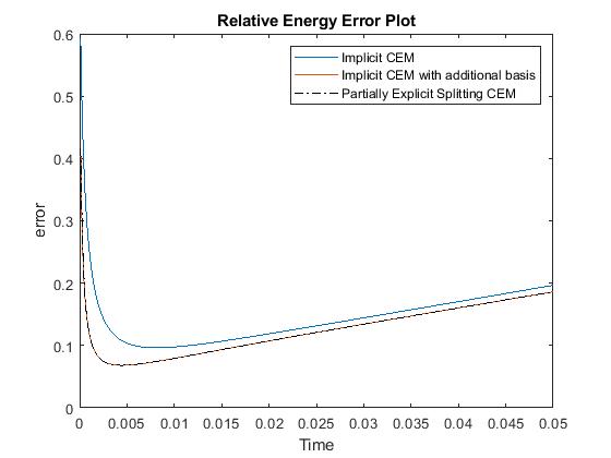
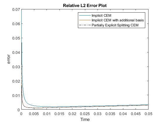
In Figure 6.1, the permeability field $\kappa$ and $g_{0}$ are presented. As is shown, this permeability field has heterogeneous high contrast channels and $g_{0}$ is a singular source term. In Figure 6.2, we first present the reference solution which is implicitly solved using fine grid basis functions. The middle plot in Figure 6.2 is implicit CEM solution obtained with additional basis functions and the solution in the right plot is obtained using the partially explicit scheme presented above. These three plots all show the solution at $t=T$ . We present two relative error plots in Figure 6.3. The first one is the relative $L^{2}$ error plot and the second one is the relative energy error plot. The blue, red and black curves (in both plots) stand for the relative error for implicit CEM solution, implicit CEM solution (with additional basis) and partially explicit solution respectively. In each of these two plots, there is a noticeable improvement for error when we use additional basis functions. We find that the black curve coincides with the red curve, which means that the partially explicit scheme can achieve similar accuracy as the fully implicit scheme.

Refer to caption — Figure 6.1: Left: $\kappa$ . Right: $g_{0}$ .

In this case,

g(u)=-(10\cdot u\cdot(u^{2}-1)+g_{0}).

The difference is that we use a smooth source term. In Figure 6.4, the permeability field $\kappa$ and source term $g_{0}$ are shown. The reference solution at the final time, implicit CEM solution (with additional basis) at the final time and partially explicit solution at the final time are presented in Figure 6.5. We show the relative $L^{2}$ error plot and the relative energy error plot in Figure 6.6. We see that the relative $L^{2}$ and energy error curves for implicit CEM (with additional basis) and partially explicit scheme almost coincide, which implies similar accuracy between them.

In our third test,

g(u)=-(10\cdot u\cdot(u^{2}-1)+g_{0}),

and we use a more complicated permeability field with more high contrast channels. Figure 6.7 shows the permeability field $\kappa$ and source term $g_{0}$ . The reference solution at $t=T$ , implicit CEM solution (with additional basis) at $t=T$ and partially explicit solution at $t=T$ are presented in Figure 6.8. In Figure 6.9, we show the relative $L^{2}$ error plot and the relative energy error plot. In this case, in both error plots, the curves for implicit CEM (with additional basis) and partially explicit scheme coincide.

In this example,

g(u)=-(10\cdot u\cdot(u^{2}-1)+g_{0}).

We use the more complicated permeability field and the smooth source term which are shown in Figure 6.10. In Figure 6.11, the reference solution at the final time, implicit CEM solution (with additional basis) at the final time and partially explicit solution at the final time are presented. Relative $L^{2}$ error and energy error plots are shown in Figure 6.12. In this case, the relative error for implicit CEM scheme is small and comparable to the two schemes with additional basis. From Figure 6.12, we can find that the $L^{2}$ and energy error for implicit CEM (with additional basis) and partially explicit scheme are nearly the same.

In this case, we use a new reaction term

g=-(1+\cos(a_{1}\cdot u)+g_{0}),\;a_{1}(x,y)=2\cos(20\pi x)\cos(20\pi y).

In numerical experiments, we set $a_{1}$ to be constant inside every fine element. Figure 6.13 shows the permeability field $\kappa$ , the source term $g_{0}$ and the function $a_{1}$ . The reference solution, implicit CEM solution (with additional basis) and partially explicit solution at the final time are shown in Figure 6.14. The relative $L^{2}$ error plot and relative energy error plot are presented in Figure 6.15. From the relative $L^{2}$ error plot, we find that the relative $L^{2}$ error for three schemes are comparable. For the relative energy error, we can find a large improvement when we introduce additional basis. The relative energy error for implicit CEM solution (with additional basis) and partially explicit solution are nearly the same.

In this case,

g=-(1+\cos(a_{1}\cdot u)+g_{0}),\;a_{1}(x,y)=2\cos(20\pi x)\cos(20\pi y).

The permeability field $\kappa$ , the source term $g_{0}$ and the funciotn $a_{1}$ are presented in Figure 6.16. The reference solution, implicit CEM solution (with additional basis) and partially explicit solution at the final time are shown in Figure 6.17. We present the relative $L^{2}$ error plot and the relative energy error plot in Figure 6.18. We observe that the $L^{2}$ and energy error curves for implicit CEM (with additional basis) and partially explicit scheme coincide.

6.3 Nonlinear $f(u)$

We want to explore the case in which the diffusion operator is nonlinear. So in Equation $(\ref{eq1})$ , we set

f(u)=-\nabla\cdot(\kappa\alpha(u)\nabla u).

Equation $(\ref{eq1})$ becomes

\displaystyle u_{t}-\nabla\cdot(\kappa\alpha(u)\nabla u)+g(u)=0.

(6.7)

Let $u_{h}$ be the fine mesh solution for Equation $(\ref{eq72})$ . We use the Picard-Newton iteration to solve the implicit equation.

\Big{(}\frac{u^{n+1,m+1}_{h}-u^{n}_{h}}{\Delta t},v\Big{)}+\int_{\Omega}\kappa\alpha(u^{n+1,m}_{h})\nabla u^{n+1,m+1}_{h}\cdot\nabla v+(g(u^{n+1,m+1}_{h}),v)=0\quad\forall v\in V_{h},

where $m$ is the Picard-Newton step number and $(\cdot,\cdot)$ is the $L^{2}$ inner product. In finite element methods, let $\{\varphi_{i}\}_{i}$ be fine mesh basis functions. We have $u^{n+1,m+1}_{h}=\sum\limits_{i}U^{n+1,m+1}_{h,i}\varphi_{i}$ , $u^{n+1,m}_{h}=\sum\limits_{i}U^{n+1,m}_{h,i}\varphi_{i}$ and $u^{n}_{h}=\sum\limits_{i}U^{n}_{h,i}\varphi_{i}$ . Let $M$ be the mass matrix. Let $U^{n+1,m+1}_{h}=(U^{n+1,m+1}_{h,i})$ , $U^{n+1,m}_{h}=(U^{n+1,m}_{h,i})$ and $U^{n}_{h}=(U^{n}_{h,i})$ . We define

\displaystyle Q(U^{n+1,m}_{h})=MU^{n+1,m}_{h}+\Delta t\cdot\mathcal{A}U^{n+1,m}_{h}-MU^{n}_{h}+\Delta t\cdot\mathcal{G},

where $\mathcal{A}=(\mathcal{A}_{ij})$

\mathcal{A}_{ij}=\int_{\Omega}\kappa\alpha(u^{n+1,m}_{h})\nabla\varphi_{j}\nabla\varphi_{i}

and $\mathcal{G}=(\mathcal{G}_{i})$

\mathcal{G}_{i}=(g(u^{n+1,m}_{h}),\varphi_{i}).

Then

(JQ)(U^{n+1,m}_{h})=M+\Delta t\mathcal{A}+\Delta t\cdot(J\mathcal{G}),

where $J\mathcal{G}=((J\mathcal{G})_{ij})$

(J\mathcal{G})_{ij}=\frac{\partial(g(u^{n+1,m}_{h}),\varphi_{i})}{\partial U^{n+1,m}_{h,j}}.

Thus,

U^{n+1,m+1}_{h}=U^{n+1,m}_{h}-(JQ)^{-1}(U^{n+1,m}_{h})Q(U^{n+1,m}_{h}).

Newton’s method for coarse mesh is similar. For the partially explicit scheme, we use the following Picard-Newton iteration which can be solved similarly using the method introduced above. Note that we change the reaction term to be partially explicit.

	$\displaystyle(\frac{u^{n+1,m+1}_{H,1}-u^{n}_{H,1}}{\Delta t}+\frac{u^{n}_{H,2}-u^{n-1}_{H,2}}{\Delta t},v_{1})+\int_{\Omega}\kappa\alpha(u^{n+1,m}_{H,1}+u^{n}_{H,2})\nabla(u^{n+1,m+1}_{H,1}+u^{n}_{H,2})\cdot\nabla v_{1}$
	$\displaystyle=(-g(u^{n+1,m+1}_{H,1}+u^{n}_{H,2}),v_{1})\quad\forall v_{1}\in V_{H,1},$
	$\displaystyle(\frac{u^{n+1}_{H,2}-u^{n}_{H,2}}{\Delta t}+\frac{u^{n}_{H,1}-u^{n-1}_{H,1}}{\Delta t},v_{2})+\int_{\Omega}\kappa\alpha(u^{n+1}_{H,1}+u^{n}_{H,2})\nabla(u^{n+1}_{H,1}+u^{n}_{H,2})\cdot\nabla v_{2}$
	$\displaystyle=(-g(u^{n+1}_{H,1}+u^{n}_{H,2}),v_{2})\quad\forall v_{2}\in V_{H,2}.$

In the following three examples, we use $g(u_{H,1}^{n+1}+u_{H,2}^{n})$ in the partially explicit algorithm. One can prove its stability as in Lemma 4.1 and Lemma 4.2. The proof is similar and we omit it here.
In the following three cases,

g(u)=-(10u(u^{2}-1)+g_{0}).

In the first example, we consider $\alpha(u)=1+u^{2}$ and time step $\Delta t=\frac{T}{500}=10^{-4}$ . The permeability field $\kappa$ and the source term $g_{0}$ are presented in Figure 6.19. The reference solution, implicit CEM solution (with additional basis) and partially explicit solution at the final time are shown in Figure 6.20. We present the relative $L^{2}$ error plot and relative energy error plot in Figure 6.21. We can find that the curves for implicit CEM solution (with additional basis) and partially explicit solution coincide, which implies that our new partially explicit scheme is also effective and has similar accuracy as the implicit CEM (with additional basis) scheme.

In this second example, we consider $\alpha(u)=2+\cos(u)$ and time step $\Delta t=\frac{0.05}{1500}$ . Figure 6.22 shows the permeability field $\kappa$ and the source term $g_{0}$ . The reference solution, implicit CEM solution (with additional basis) and partially explicit solution at $t=T$ are presented in Figure 6.23. The relative $L^{2}$ error plot and relative energy error plot are shown in Figure 6.24. The partially explicit scheme also works in this case and has similar accuracy as the implicit CEM (with additional basis) scheme.

In this case, we have $\alpha(u)=2+\cos(u)$ and time step $\Delta t=\frac{0.05}{1500}$ . The permeability field $\kappa$ and the source term $g_{0}$ are presented in Figure 6.25. We show the reference solution, implicit CEM solution (with additional basis) and partially explicit solution at $t=T$ in Figure 6.26. The relative $L^{2}$ error plot and the relative energy error plot are presented in Figure 6.27. From Figure 6.27, we see that the curves for implicit CEM (with additional basis) and partially explicit scheme coincide, which implies that they have similar accuracy.

7 Conclusions

In this work, we design and analyze contrast-independent time discretization for nonlinear problems. The work continues our earlier works on linear problems, where we propose temporal splitting and associated spatial decomposition that guarantees a stability. We introduce two spatial spaces, the first account for spatial features related to fast time scales and the second for spatial features related to “slow” time scales. We propose time splitting, where the first equation solves for fast components implicitly and the second equation solves for slow components explicitly. We introduce a condition for multiscale spaces that guarantees stability of the proposed splitting algorithm. Our proposed method is still implicit via mass matrix; however, it is explicit in terms of stiffness matrix for the slow component. We present numerical results, which show that the proposed methods provide very similar results as fully implicit methods using explicit methods with the time stepping that is independent of the contrast.

Acknowledgments

The research of Eric Chung is partially supported by the Hong Kong RGC General Research Fund (Project numbers 14304719 and 14302018) and the CUHK Faculty of Science Direct Grant 2020-21.

References

[1] A. Abdulle. Explicit methods for stiff stochastic differential equations. In Numerical Analysis of Multiscale Computations, pages 1–22. Springer, 2012.
[2] G. Ariel, B. Engquist, and R. Tsai. A multiscale method for highly oscillatory ordinary differential equations with resonance. Mathematics of Computation, 78(266):929–956, 2009.
[3] U. M. Ascher, S. J. Ruuth, and R. J. Spiteri. Implicit-explicit Runge-Kutta methods for time-dependent partial differential equations. Applied Numerical Mathematics, 25(2-3):151–167, 1997.
[4] J. Bear. Dynamics of fluids in porous media. Courier Corporation, 2013.
[5] D. L. Brown, Y. Efendiev, and V. H. Hoang. An efficient hierarchical multiscale finite element method for stokes equations in slowly varying media. Multiscale Modeling & Simulation, 11(1):30–58, 2013.
[6] E. T. Chung, Y. Efendiev, and T. Hou. Adaptive multiscale model reduction with generalized multiscale finite element methods. Journal of Computational Physics, 320:69–95, 2016.
[7] E. T. Chung, Y. Efendiev, and C. Lee. Mixed generalized multiscale finite element methods and applications. SIAM Multiscale Model. Simul., 13:338–366, 2014.
[8] E. T. Chung, Y. Efendiev, and W. T. Leung. Generalized multiscale finite element methods for wave propagation in heterogeneous media. Multiscale Modeling & Simulation, 12(4):1691–1721, 2014.
[9] E. T. Chung, Y. Efendiev, and W. T. Leung. Constraint energy minimizing generalized multiscale finite element method. Computer Methods in Applied Mechanics and Engineering, 339:298–319, 2018.
[10] E. T. Chung, Y. Efendiev, and W. T. Leung. Constraint energy minimizing generalized multiscale finite element method in the mixed formulation. Computational Geosciences, 22(3):677–693, 2018.
[11] E. T. Chung, Y. Efendiev, and W. T. Leung. Fast online generalized multiscale finite element method using constraint energy minimization. Journal of Computational Physics, 355:450–463, 2018.
[12] E. T. Chung, Y. Efendiev, W. T. Leung, M. Vasilyeva, and Y. Wang. Non-local multi-continua upscaling for flows in heterogeneous fractured media. Journal of Computational Physics, 372:22–34, 2018.
[13] J. Du and Y. Yang. Third-order conservative sign-preserving and steady-state-preserving time integrations and applications in stiff multispecies and multireaction detonations. Journal of Computational Physics, 395:489–510, 2019.
[14] L. Duchemin and J. Eggers. The explicit–implicit–null method: Removing the numerical instability of pdes. Journal of Computational Physics, 263:37–52, 2014.
[15] W. E and B. Engquist. Heterogeneous multiscale methods. Comm. Math. Sci., 1(1):87–132, 2003.
[16] Y. Efendiev, J. Galvis, and T. Hou. Generalized multiscale finite element methods (GMsFEM). Journal of Computational Physics, 251:116–135, 2013.
[17] Y. Efendiev, J. Galvis, G. Li, and M. Presho. Generalized multiscale finite element methods. nonlinear elliptic equations. Communications in Computational Physics, 15(3):733–755, 2014.
[18] Y. Efendiev and T. Hou. Multiscale Finite Element Methods: Theory and Applications, volume 4 of Surveys and Tutorials in the Applied Mathematical Sciences. Springer, New York, 2009.
[19] Y. Efendiev and A. Pankov. Numerical homogenization of monotone elliptic operators. SIAM J. Multiscale Modeling and Simulation, 2(1):62–79, 2003.
[20] Y. Efendiev and A. Pankov. Homogenization of nonlinear random parabolic operators. Advances in Differential Equations, 10(11):1235–1260, 2005.
[21] W. Ehlers. Darcy, forchheimer, brinkman and richards: classical hydromechanical equations and their significance in the light of the tpm. Archive of Applied Mechanics, pages 1–21, 2020.
[22] B. Engquist and Y.-H. Tsai. Heterogeneous multiscale methods for stiff ordinary differential equations. Mathematics of computation, 74(252):1707–1742, 2005.
[23] W. T. L. Eric Chung, Yalchin Efendiev and P. N. Vabishchevich. Contrast-independent partially explicit time discretizations for multiscale flow problems. arXiv:2101.04863.
[24] W. T. L. Eric Chung, Yalchin Efendiev and P. N. Vabishchevich. Contrast-independent partially explicit time discretizations for multiscale wave problems.
[25] J. Frank, W. Hundsdorfer, and J. Verwer. On the stability of implicit-explicit linear multistep methods. Applied Numerical Mathematics, 25(2-3):193–205, 1997.
[26] P. Henning, A. Målqvist, and D. Peterseim. A localized orthogonal decomposition method for semi-linear elliptic problems. ESAIM: Mathematical Modelling and Numerical Analysis, 48(5):1331–1349, 2014.
[27] T. Hou and X. Wu. A multiscale finite element method for elliptic problems in composite materials and porous media. J. Comput. Phys., 134:169–189, 1997.
[28] T. Y. Hou, D. Huang, K. C. Lam, and P. Zhang. An adaptive fast solver for a general class of positive definite matrices via energy decomposition. Multiscale Modeling & Simulation, 16(2):615–678, 2018.
[29] T. Y. Hou, Q. Li, and P. Zhang. Exploring the locally low dimensional structure in solving random elliptic pdes. Multiscale Modeling & Simulation, 15(2):661–695, 2017.
[30] T. Y. Hou, D. Ma, and Z. Zhang. A model reduction method for multiscale elliptic pdes with random coefficients using an optimization approach. Multiscale Modeling & Simulation, 17(2):826–853, 2019.
[31] W. Hundsdorfer and S. J. Ruuth. Imex extensions of linear multistep methods with general monotonicity and boundedness properties. Journal of Computational Physics, 225(2):2016–2042, 2007.
[32] G. Izzo and Z. Jackiewicz. Highly stable implicit–explicit runge–kutta methods. Applied Numerical Mathematics, 113:71–92, 2017.
[33] P. Jenny, S. Lee, and H. Tchelepi. Multi-scale finite volume method for elliptic problems in subsurface flow simulation. J. Comput. Phys., 187:47–67, 2003.
[34] C. Le Bris, F. Legoll, and A. Lozinski. An MsFEM type approach for perforated domains. Multiscale Modeling & Simulation, 12(3):1046–1077, 2014.
[35] T. Li, A. Abdulle, et al. Effectiveness of implicit methods for stiff stochastic differential equations. In Commun. Comput. Phys. Citeseer, 2008.
[36] G. I. Marchuk. Splitting and alternating direction methods. Handbook of numerical analysis, 1:197–462, 1990.
[37] M. Narayanamurthi, P. Tranquilli, A. Sandu, and M. Tokman. Epirk-w and epirk-k time discretization methods. Journal of Scientific Computing, 78(1):167–201, 2019.
[38] H. Owhadi and L. Zhang. Metric-based upscaling. Comm. Pure. Appl. Math., 60:675–723, 2007.
[39] A. Roberts and I. Kevrekidis. General tooth boundary conditions for equation free modeling. SIAM J. Sci. Comput., 29(4):1495–1510, 2007.
[40] S. J. Ruuth. Implicit-explicit methods for reaction-diffusion problems in pattern formation. Journal of Mathematical Biology, 34(2):148–176, 1995.
[41] G. Samaey, I. Kevrekidis, and D. Roose. Patch dynamics with buffers for homogenization problems. J. Comput. Phys., 213(1):264–287, 2006.
[42] H. Shi and Y. Li. Local discontinuous galerkin methods with implicit-explicit multistep time-marching for solving the nonlinear cahn-hilliard equation. Journal of Computational Physics, 394:719–731, 2019.
[43] P. N. Vabishchevich. Additive Operator-Difference Schemes: Splitting Schemes. Walter de Gruyter GmbH, Berlin, Boston, 2013.

Contrast-independent partially explicit time discretizations for nonlinear multiscale problems

Abstract

1 Introduction

2 Problem Setting

3 Discretization

4 Partially explicit scheme with space splitting

Energy stability

Lemma 4.1.

Proof.

Lemma 4.2.

Proof.

5 Discussions

5.1 G=0G=0 case

5.2 G≠0G\not=0 case.

6 Numerical Results

6.1 VH,1V_{H,1} and VH,2V_{H,2} constructions

6.1.1 CEM method

6.1.2 Construction of VH,2V_{H,2}

6.2 Linear f​(u)f(u)

6.3 Nonlinear f​(u)f(u)

7 Conclusions

Acknowledgments

References

5.1 $G=0$ case

5.2 $G\not=0$ case.

6.1 $V_{H,1}$ and $V_{H,2}$ constructions

6.1.2 Construction of $V_{H,2}$

6.2 Linear $f(u)$

6.3 Nonlinear $f(u)$