Continuations and bifurcations of relative equilibria for the positive curved three body problem
Abstract
The positive curved three body problem is a natural extension of the planar Newtonian three body problem to the sphere . In this paper we study the extensions of the Euler and Lagrange Relative equilibria ( in short) on the plane to the sphere.
The on are not isolated in general. They usually have one-dimensional continuation in the three-dimensional shape space. We show that there are two types of bifurcations. One is the bifurcations between Lagrange and Euler . Another one is between the different types of the shapes of Lagrange . We prove that bifurcations between equilateral and isosceles Lagrange exist for equal masses case, and that bifurcations between isosceles and scalene Lagrange exist for partial equal masses case.
Toshiaki Fujiwara1, Ernesto Pérez-Chavela2
1College of Liberal Arts and Sciences, Kitasato University, Japan. [email protected]
2Department of Mathematics, ITAM, México.
Keywords Relative equilibria, Euler configurations, Lagrange configurations, cotangent potential.
Math. Subject Class 2020: 70F07, 70F10, 70F15
1 Introduction
A relative equilibrium for the Newtonian –body problem, is a particular solution where the masses are rotating uniformly around their center of mass with the same angular velocity. In these kind of motions the masses preserve their mutual distances for all time, that is, they behave as a rigid body motion. The fixed configuration at any time is called a central configuration. In the corresponding rotating frame they form an equilibrium point, from here the name [22, 17].
Since the central configurations are invariant under rotations and homotheties, we count classes of central configurations modulo these Euclidean transformations; then for , there are only 5 classes of relative equilibria, three collinear or Euler relative equilibria [10] and two equilateral triangle or Lagrange relative equilibrium [16].
The curved –body problem is a natural extension of the classical Newtonian problem to spaces of constant curvature which could be positive or negative. For , the problem is divided into two classes, the Kepler problem (one particle is fixed, and the other one is moving according to it) and the –body problem (both masses are moving according to their mutual attractions). The first one is an old problem, introduced independently in the 1830’s by J. Bolyai and N. Lovachevsky the codiscovers of the first non-Euclidean geometries. The second one was introduced by Borisov et al [4, 5]. Unlike the Newtonian problem, on the sphere these problems are not equivalent, the first one is integrable and the second one is not [20].
In 1994, V.V. Kozlov showed that the cotangent potential is the natural way to extend the Newtonian potential to spaces of constant positive curvature [13]. In 2012, F. Diacu, E. Perez-Chavela and M. Santoprete [6], obtained the generalization of this problem in an unified way for any value of and any value of the constant curvature . You can see [7] and [5] for a nice historical description of this problem.
In this paper we are interested in the analysis of relative equilibria for the two dimensional positive curved three body problem, which can be reduced to the analysis on the unit sphere . That is, we will study relative equilibria for three positive masses moving on under the influence of the cotangent potential. From here on, just to simply the notation we call to the relative equilibria simply as .
By exploiting the symmetries of some configurations and using spherical trigonometric arguments, several authors have found different families of on the sphere see for instance [6, 7, 8, 9, 18, 19, 21, 23].
In a recent paper [11], the authors of this article developed a new systematic geometrical method to study on , where the masses are moving on the sphere under the influence of a potential which only depends on the mutual distances among the masses, in particular for the cotangent potential. For the authors divide the analysis of on in two big classes, the Euler relative equilibria ( by short) where the three masses are on the same geodesic, and the Lagrange relative equilibria ( by short), for the which are not in the previous class. In the same paper [11], the authors find the necessary and sufficient conditions on the shapes, to obtain and . In this paper we will restrict our analysis to the cotangent potential, that is, to the positive curved three body problem.
In [1], the authors proved that any of the planar –body problem can be continued to spaces of constant curvature , positive or negative for small values of the parameter . This is a remarkable result, because for instance, it is well known that any three masses located at the vertices of an equilateral triangle generate a on the plane; however in the case of curved spaces, with equilateral triangle shape only exist if the three masses are equal. In particular they show that any Lagrange relative equilibria can be continued to the sphere (the equilateral triangle shape, is not preserved in the continuation if the masses are not equal).
In this paper we will show that in general, we can continue a on the sphere, represented by an one dimensional curve. When two continuations of intersect, we call it a bifurcation, in the next section we will give the precise definition of these concepts.
After the introduction, the paper is organized as follows: In Section 2 we give the definitions of all concepts used along the paper, and we show how use the implicit function theorem to find the bifurcation points and the extensions of solutions. In Section 3 we do the analysis for the case of equal masses and in Section 4 we do the analysis for the case of partial equal masses. In section 5, we study with general masses, and finally in Section 6 we summarize our results and state some final comments.
2 Conditions for a Shape
We consider three positive masses denoted by moving on a sphere of radius that we denote as . The equations of motions are described by the Lagrangian, which in spherical coordinates take the form,
| (1) |
To facilitate the notations, we set unless otherwise specified. We denote the angle of the minor arc on the great circle connecting the masses and as . In order to avoid singularities, we exclude the case , which corresponds to
The above angles are related to each other by the relationship
| (2) |
For the three-body problem, it is convenient to use the notation for and . We define
| (3) |
The inequalities in are the conditions of to form a triangle. Note that one point in corresponds to two triangles with opposite orientation.
Definition 1.
A relative equilibrium is a solution of the equations of motion, which in spherical coordinates satisfies
That is, a solution that behaves as if the masses belonged to a rigid body, the shape is the same for all time.
Remark 1.
Usually, people working on Geometric Mechanics define the as fixed points in a reduced system (see for instance [14] and the references therein). In other words, the are solutions which are invariant under the action of a continuous symmetric group . In our case the symmetric group is . The correspond to periodic orbits in the original phase space (the not reduced one), these periodic orbits are rotating uniformly around a principal axis. Then in order to determine a , we need to have the initial configuration and the angular velocity. If we express these conditions in the usual spherical coordinates, taking the rotation axis as the –axis, we obtain Definition 1. By the other hand, if Definition 1 holds, then since , we obtain that a is a fixed point in the reduced system. So, both definitions are equivalent.
As we have seen in the previous Section, there are two kinds a on the sphere, and . In [11], we proved that the must be on the equator or on a rotating meridian.
The big difficulty to study on the sphere is that the linear momentum and the center of mass are not more a first integral for the positive curved problem.
Fortunately in [11], we found that the center of mass can be substitute by the vanishing of two components of the angular momentum on the sphere.
To verify this fact, we observe that the Lagrangian is invariant under rotations around the centre of , the angular momentum vector is a first integral. The components of are
Then, fixing the rotation axis as the –axis, we obtain that the components and are integrals of motion.
Now by Definition 1, after the substitution and , the angular momentum has the form where
| (4) | ||||
We observe that taking finite, in the limit we obtain , since for . Then, using equation (4), the expansion for and and dropping the higher order terms we obtain
| (5) |
Finally using the fact that , the above equation (5), is the condition to fix the center of mass at the origin on the Euclidean plane (see [11] for more details).
Remark 2.
In [4] the authors use the reduction method to guarantee that the projections of the angular momentum of the system onto the original space are preserved. Then by using Noether’s theorem, they obtain the expressions of the above projections in Euler’s angles. Due to the more classical geometric viewpoint that we discuss along this manuscript, we prefer to use our approach.
Using the two integrals and , we prove that the problem to find on is reduced to solve the eigenvalue problem where is an useful representation of the inertia tensor given by (see [11] for more details)
| (6) |
In the same paper [11], we show that the necessary and sufficient conditions to have or , can be described only in terms of and , . The conditions for a shape to form are
| (7) |
Let be the difference of and , namely
| (8) |
Then, the condition for have a is equivalent to .
The correspondence between the solution of this condition and the configuration variables is given by
| (9) |
Then using and , equation (2) determines . Where is the total mass, and . If we take the three masses are on the northern hemisphere, when they are on southern hemisphere. Finally, the angular velocity is given by
| (10) |
Thus, the problem to find a configuration of is reduced to find the solution of the condition (See [11] for more details).
Similarly, the necessary and sufficient condition for a shape to form an on a rotating meridian with , namely the mass is located between and , is
| (11) |
You can consult reference [11] for the correspondence between and the configuration variables , .
The conditions for a shape to form an on the equator are
| (12) |
where . For this case, is given by
| (13) |
Note that there is just one set of ’s (two shapes with different orientation) for given masses. For the and the on a rotating meridian on the sphere, we will show that some of these can be continued into the three dimensional space given by , and that these continuations can meet in this space. We call this “bifurcation”, to be more precise we define:
Definition 2.
A bifurcation point of and on a rotating meridian is a point on a plane , where the continuation of a and an coincide. This bifurcation point is a coupling where two continuations of with opposite orientation connected.
We will show ahead in this paper, that some meets on the equator, and since an on the equator is just one point for given mass ratio and given orientation, we define:
Definition 3.
An Euler coupling on the Equator is a point with , where two continuations of with the same orientation, one on the northern and the other one on the southern hemisphere, connected.
Finally we have that the shapes of can be grouping into equilateral, isosceles, and scalene triangles. We will show that for equal masses case, , equilateral and isosceles have continuation. When only two masses are equal, for instance , we have continuation of isosceles and scalene . We define the bifurcation point as follows.
Definition 4.
Let the set be one of {equilateral, isosceles} or {isosceles, scalene} . A bifurcation point between and is the intersection point of the continuation of and .
The existence of bifurcation points between one in the group and other in the group can be understood by two simple but important properties of the surfaces defined by in .
Property 1.
For ,
| (14) |
From this property we obtain the following proposition and corollaries whose proofs are obvious.
Proposition 1.
The necessary condition for with is
Corollary 1.
Unequal masses implies scalene triangle .
Corollary 2.
Equilateral triangle needs .
Property 2.
For , the function is an anti-symmetric function of and , and can be factorized as
| (15) |
where
| (16) |
This property explains the existence of bifurcation points between two groups of shapes of .
We explain why for we obtain a bifurcation point of isosceles and scalene . For this case, the surface is split into the plane , and the surface by Property 2. Then, the condition for , , is split into two cases, intersection of and namely isosceles , and intersection of and , namely scalene . Then, the intersection of the three surfaces and and gives the bifurcation points.
Similarly, there are bifurcation points of equilateral and isosceles for the equal masses case, .
We will use the implicit function theorem to study bifurcations. By this theorem, if two continuous differentiable functions and have a solution , and at , then a continuation of the solution from this point exists in some finite interval. A geometrical interpretation of this theorem is that the conditions and means that the two surfaces intersect at this point and the vector represents the tangent vector of the intersection curve at this point.
3 Equal masses case
As shown in Property 2, the conditions for have a , and are split into ( or ) and ( or ).
First we will show that there are no scalene (intersection of and ), then we describe the equilateral ( and ) and isosceles ( and or and ) and the bifurcation between them.
3.1 No scalene
Theorem 1.
There are no scalene for the equal masses case.
Proof.
We will show a contradiction if we assume that there is a scalene with . Let be , then and . Since, this is a scalene triangle, must satisfies . By the definition of the function , it is symmetric for the first two variables. Therefore, must be zero for any permutation of if the assumption is true.
Now, define and for by
| (17) |
Since for any permutations of and , for any permutations of . Similarly, . Here, the function is a totally symmetric function of ,
| (18) |
The possible solutions of are or or . However
| (19) |
Similarly , and . This is the contradiction we are looking for. ∎
3.2 Isosceles and equilateral
In this subsection, we consider the shape with . So,
| (20) |
The isosceles solution is the solution of
| (21) |
Obviously .
Proposition 2.
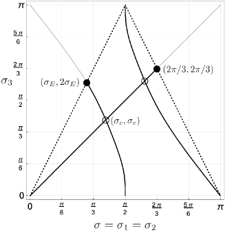
The bifurcation points between equilateral and isosceles are and , where (see Figure 1).
Proof.
The bifurcation points are the solutions of
| (22) |
. ∎
Proposition 3.
The end points of an equilateral , , , is the on the equator. The end point of isosceles , with
| (23) |
is the on a rotating meridian.
Proof.
The former is obvious. The latter is the solution of
| (24) |
∎
The point is the bifurcation point between isosceles and on a rotating meridian. We will consider this bifurcation point in the next section.
4 Partial equal masses case
In this section, we consider the case , with .
As shown in Property 2, the condition is reduced to or . In the next subsection, we consider the first case, isosceles (intersection of and ). The subsection 4.1.2 is devoted to the bifurcation of isosceles and isosceles . The second case, ( and ) describes scalene . In subsection 4.2, we will treat the bifurcation of isosceles and scalene ( and and ).
4.1 Isosceles
Let be , then and take the same form as in (20).
4.1.1 Mass ratio for a given shape
Let be
| (25) | |||||
| (26) |
A simple calculation proves that the solutions of are, the point in , and the points and on the boundary of . Where, is defined by (23). See Figure 2.

Then the following proposition follows.
Proposition 4.
For , any point in with forms an isosceles by choosing suitable .
Proof.
For this case, is satisfied. Therefore, the condition for is
| (27) |
Therefore, if and ,
| (28) |
This equation defines in terms of uniquely, and demands . In fact, the region in is the region where and . ∎
The next result follows inmediatly from equation (27).
Proposition 5.
The shape that makes satisfies the condition for for any .
Actually this shape is an on a rotating meridian. Therefore, it corresponds to the bifurcation point of and , that is, we can pass from a to an or vice versa.
Proposition 6 (Euler coupling).
On the line , only satisfies the condition for with any . On the other hand, on the line , any point in satisfies the condition for choosing suitable .
Proof.
On the line , and . Therefore, if , and if .
On the other hand, on the line , and . Therefore because . For this case, . This shape is the on the equator. And the inequality is exactly the same as the condition (12) for on the equator. ∎
4.1.2 Bifurcation point between isosceles and isosceles
Proposition 7.
The shape is the unique bifurcation point between isosceles and isosceles .
Proof.
In the previous Proposition we have already proved that the shape is the Euler coupling of isosceles . Obviously, the shape is an on the rotating meridian, and then, continuation from this shape of isosceles for any does exist.
The proof of the existence of the continuation of a for any is given by showing that . In fact,
| (29) |
By the implicit function theorem, there is a continuation of from . ∎
4.1.3 Isosceles for the restricted three-body problem
Here we consider the isosceles in the restricted problem with finite and . The size dependence will be interesting.
The isosceles for this limit are represented by the curve in Figure 2, since . As we can see, there are two curves where , one connects and , and the other connects and .
Now, trace the isosceles with respect to . For sufficiently small , there is one shape that is almost equilateral. Note that one shape in represents four configurations, two for orientations of the triangle, and two for the places near the north pole or south pole. So, there are four configurations for . Then at , new shape bifurcated from . So, there are eight configurations for .
With respect to , the situation is more complex. Note that the graph takes the local minimum and maximum for at , where the minimum and maximum value of are the solution of . The solutions are (the local maximum), and (the local minimum). So, the range is divided into four pieces by the three values . As shown in Figure 2, in the interval , there are no isosceles for the restricted problem.
4.2 Bifurcation points between isosceles and scalene
In this subsection, we will show the existence of the bifurcations between isosceles with and scalene . As described in the section 2, the bifurcation point of this type is the intersection of three surfaces, , , and .
Now, since
| (30) |
we obtain that is equivalent to
| (31) |
On the other hand, determines by equation (28). Substituting this into the equation (31), we get the equation for the set of and ,
| (32) |
Unfortunately, we don’t have a proof that almost all points on the curve have a continuation of scalene . But we are able to give a proof for two points.
Example 1.
The points and are bifurcation points between isosceles and scalene .
Proof.
It is not difficult to verify that the points and satisfy the condition . In fact the point corresponds to an isosceles for . For , the vector indicates the scalene direction, and the vector indicates the isosceles direction. By the implicit function theorem, there are continuation of scalene and isosceles from .
Similarly, corresponds to an isosceles for . In this case the corresponding vectors are and . ∎
In subsection 4.3.2, we will give a numerical result that shows that there are continuation of scalene from the points on except for three exceptional points.
4.3 Numerical results
In this subsection we present numerical simulations which show some continuations of .
4.3.1 Isosceles

The result of the numerical calculations are shown in Figure 3. The contours represent curves for a positive constant. The white region in this figure represents . The gray region is or outside of . Every contour with has a unique continuation from an edge to another edge of .
The - continuations for are emerging from the origin as showed above, it looks close to a straight line. The end points of this continuation are for , and (binary collision) for .
Figure 3 shows that the continuation of for any are emerging form , which is the unique bifurcation point between and for case.
4.3.2 Bifurcation between isosceles and scalene

Figure 4 shows two examples of bifurcations between isosceles and scalene for which were described in Example 1. For each mass ratio, two bifurcation pints exists. For , the continuation of scalene is a closed loop as shown in the left side of figure 4. The loop intersects one continuation curve of the isosceles continuation twice. This isosceles continuation is the - continuation. For , we also get two bifurcation points. In this case, two scalene continuation curves intersect two different continuation of isosceles curves. See the right side of Figure 4.
Figure 5 shows the global structure of the bifurcation point of this type. The points on the curve give the bifurcation points if . The curve is also shown in the same figure.

We can see in this figure, that the bifurcations occur for sufficiently small. That is, the bifurcation from - continuation is only possible if with sufficiently small . In the following we will show numerically how small could be .
On the cross point of and the bifurcation doesn’t occur, namely, no continuation of scalene solutions exists. Figure 5 shows that there are three such points. The points , , correspond to the bifurcation points for equilateral and isosceles for . The other point is new. The mass ratio at this point is . Numerical calculations suggest that this point is the lower bound for , where we can find bifurcation to scalene from the - continuation. In other words, the bifurcation of this type occurs for . The reason is the following. At , the scalene continuation is a loop. This means that two surfaces of and intersect, and the intersection curve is a loop. Numerical calculation shows that smaller makes smaller loop, and at the limit the loop becomes just a point . Namely, the two surfaces just touch at this point. Thus the lower bound for in order to have this kind of bifurcation is .
5 with general masses
In this section, we will tackle the case of general masses. Remember that if the three masses are not equal, by Corollary 1, the shapes for the are scalene triangles.
5.1 Continuation from Lagrangian equilateral on to on
Let be the arc length between the masses and , where . Then , where is the radius of . The Euclidean limit where the Lagrange equilateral solution exists is achieved by taking .
Proposition 8.
The Lagrange equilateral solution when goes to infinity exists, and the continuation to finite also exists.
Proof.
The limit of the conditions are
| (33) |
The solution is , , which corresponds to the equilateral .
Then, for ,
| (34) |
By the implicit function theorem, the continuation of equilateral to finite exists. ∎
The above result was first proved in [1], by using a different approach.
Proposition 9.
The continuation of equilateral in to with finite has if .
Proof.
Let be . Then the expansion of to is
| (35) |
Therefore, if for sufficiently small . By Proposition 1, the ordering of cannot be changed in the continuation of the solution. Therefore, the ordering is preserved in the continuation to finite size of . ∎
Remark 4.
For finite , there are no equilateral solutions if the masses are not equal. Instead, there are almost equilateral solutions if . Similarly, there are three continuations of which are almost similar to the three Euler solutions on the Euclidean plane [11]. We call such continuation of the solutions as “ - continuation” and “ - continuations” respectively, because these continuations start from the origin.
5.2 Continuation of Euler on the equator to Lagrange
If the masses satisfy the condition (12), then on the equator exists.
Proposition 10.
The continuation of from an on the equator exists.
Proof.
Direct calculation shows that are satisfied by in (13). Besides that, we get
| (36) |
By the implicit function theorem, we get the result. ∎
Proposition 11.
The continuation of from the on the equator has if .
Proof.
Without loss of generality, we can assume that . Since for , is obvious. Then for , , and yields , because any on the equator satisfies . Since is a decreasing function in , the proposition is proved. ∎
5.3 Mass ratio for a given shape
To go further into the consideration of the bifurcation of and for general masses, we treat the conditions for , , as the equations for the mass ratios and . This subsection is an extension of the section 4.1.1 for partial equal masses case to the general masses case.
The conditions take the form
| (37) |
where is a two by three matrix in function of . The rank of is at most two.
If , is determined uniquely. Let be
| (38) |
Then
| (39) |
The following lemmas are obvious.
Lemma 1.
For a given shape , if and if the equation gives and , then this shape form a with this mass ratio.
Remark 5.
We have checked the shapes in with and . There are 73 among the total of such grid points. All of them have . There are 25 scalene . For example has , , and .
Lemma 2.
For a given shape , if and there are solutions that satisfy , then this shape form a with these mass ratios.
5.4 Bifurcations between on a rotating meridian and
If there is a bifurcation point between an on a rotating meridian and a , it must be on the plane . Without loss of generality, we can take the plane .
5.4.1 Bifurcation points on the plane
The aim of this subsection is to prove the following result.
Theorem 2.
Any point on the curve
| (40) |
which belongs to the plane is a bifurcation point of on a rotating meridian and a for continuously many . Inversely, if a continuation of (for given ) reaches the plane, the point is on the curve . Therefore, this is a bifurcation point between and .
The proof of this Theorem is given in a sequence of lemmas.
Lemma 3.
On the plane , on the curve , otherwise .
Proof.
A direct calculation shows that
| (41) |
Since , this vector is null if and only if . ∎
Lemma 4.
The curve , for , is a continuous curve that connects and . The range of is .
Proof.
Since , the solutions of are . But on these points. Therefore on . Then
| (42) |
Since
| (43) |
is a strictly increasing function of . Therefore, the upper limit of is given by . The solution is and . Decreasing , there are two solutions of . At , , and and . For the solution are out of . Therefore, the range of is . ∎
Lemma 5.
On the plane , we can find positive mass ratios that satisfy the conditions only on the curve . Outside of this curve, the conditions demand .
Proof.
On the curve , , the solutions are given by,
| (44) |
As shown above on , therefore the coefficient of in equation (44) is always positive; whereas the constant term could be positive, zero or negative. Therefore, for any point on , we can always take positive and .
On the other hand, at where , . Therefore, are determined uniquely. A direct calculation shows that both are negative,
| (45) |
∎
Remark 6.
As shown in (44), continuously many share the same on .
Lemma 6.
The shape on with the mass ratios given by equation (44) satisfies the condition for .
Proof.
Lemma 7.
For a given point on and which are related by equation (44), the continuation of from this point exists.
Proof.
The substitution of given by equation (44) into gives
| (48) |
where is a two by two matrix of functions of . Now, a direct calculation using yields
| (49) |
Therefore, if , . By the implicit function theorem, there is a continuation of from this point.
For the case , we know from by Proposition 1 that . The existence of the continuation of with is obvious. ∎
Lemma 8.
For a given point on and that are related by equation (44), the continuation of from this point exists.
Proof.
Consider at the point , where . Substituting given by equation (44), we obtain that each component of has the form , where the are functions of . Namely,
| (50) |
Substituting and using in (42), we get
| (51) |
where
| (52) |
We can show that on by a simple calculation.
Therefore, if . By the implicit function theorem, there is a continuation of from this point.
5.4.2 Number of bifurcation points on for given mass ratio
In the previous Theorem we showed that any point on the curve located on the plane is a bifurcation point between and for continuously many .
Then for given , how many bifurcation points exist on the plane, and what if exist? In this subsection, we will give an equation to count the number, and to find the position.
Substituting (42) into (44), we get
| (53) |
where , and . Then, with (42) for will determine . Then and will determine and .
Note that with (42) is a decreasing function of , which takes the value for and for . On the other hand, for and for . Therefore, it may have or solutions of .
Then, we get the following lemma.
Lemma 9.
For the case , there is at least one bifurcation point between and on the plane , .
Proof.
The denominator of has zero if . If is outside of this range, the result is obvious because is a continuous function. If is in this range, the function is not continuous but goes to plus infinity at the point. Therefore, the equation has at least one solution. ∎

Then, the following result is obvious.
Proposition 12.
For , there is at least one bifurcation point of and on the plane , .
Proof.
Without loss of generality, we can assume . Then , namely is satisfied. ∎
5.5 Numerical Results
Figure 6 shows examples of that give bifurcation points. Although the case has no bifurcation point on the plane , it has the bifurcation point on the plane by Proposition 12 because is the heaviest for this case.

The corresponding continuations of for , , and are shown in Figure 7. The grey plane corresponds to . Left: At , there is only one bifurcation point between - and -. As you can see in Fig. 7, there is a small loop near the plane, which does not reach the plane. Therefore, the loop doesn’t yields a bifurcation point. As is smaller, the loop is larger. Middle: When , the loop touches the plane at one point, which is a new bifurcation point. Thus, there are two bifurcation points for as shown in Figure 6. The bifurcated is different from the -. Decreasing the loop gets bigger and then intersects the plane. Right: Thus, we have three bifurcation points at .
In Figure 7, another similar small loop (left) and open arc (right) which bifurcate to on the plane is shown.
The continuation which starts at bifurcates to on . The end point of the continuation that starts at is on the equator.
We see other two loops that start and end at or . They are elements of the seven continuations in Figure 7, where the mass ratios are not so far from .

Figure 8 shows the continuations for and . No loop continuations are seen. Three continuations exist for . On the other hand, since the mass ratio does not satisfy the condition for on the equator (12), the and the continuation of from this point does not exist. Thus, there are only two continuations of .
The numerical experiments show a couple of interesting properties of the continuation of , , and the bifurcation between them.
(1) The - continuation and one of the - continuations are directly connected by the bifurcation point. The -continuation reaches the plane , then bifurcates to , where (the heaviest mass) is placed in the middle, Then it continues back to the - continuation keeping (the heaviest mass) in the middle. See Figures 7 and 8. Note that Proposition 12 ensures the existence of such bifurcation point between a and an continuations, but not ensures that the continuations are - and -.
(2) There are at most continuations of . Among them, the - continuation and the continuation of from on the equator sharing the same ordering of , namely if by Propositions 9 and 11. The other continuations have mutually different ordering. Therefore, all possible orderings of ’s are realised by the continuations.
6 Conclusions and final comments
The variables for having on is determined by the two conditions . Therefore, have one-dimensional intersection curve, namely one-dimensional continuation, in general. Similarly, on have one-dimensional continuation.
We have proved the local existence of the continuations. The proof for the global existence of such continuation still need a better understanding of the surfaces defined by .
Special attention was paid to the - continuation. On the Euclidean plane , there are two isolated Lagrangian equilateral configurations that have opposite orientation, and three isolated Euler configurations. We have shown that on , with almost all mass ratios, the - continuation (two almost equilateral configurations with opposite orientations) and one - continuation, where the heaviest mass is placed between the other two masses, are connected by the continuations via bifurcation(s). See Figure 9. This is true for the mass ratios and , but not true for . See the continuation in Figure 3.

When we say that there are two Lagrange equilateral solutions in the planar three-body problem, we count the similarity class of the shapes under rotations and homotheties. Since we don’t have these similarity classes on , we have continuously many as shown in Figure 9. However, the counting based on similarity has not much meaning to compare the number of solutions on and Euclidean .
It is better to count the number of on the basis of continuity instead of similarity. Because the similar shape with fixed and scaling factor is an one dimensional continuation, the continuation is a natural extension of similarity. For the continuation, we have one in the space , and two in the configuration space counting two orientations. By the same counting, we have at most seven continuations in , and continuations for configurations. Where, the first factor counts the orientations, and the second counts whether the placement is in the northern or southern hemisphere ( in equation (9)).
In this article we have considered only positive masses. Some authors have studied the case for two positive masses and a third massless particle, called the restricted three body problem on , see for instance [12, 15]. An interesting question is try to extend our results to the restricted problem. In this paper we have analyzed just the restricted isosceles on the sphere, that is, we consider and (see subsection 4.1.3). We showed that our results cover this particular case. We pointing out that in this case, there are values of not allowed for having , size shape dependence is interesting. However we are far to have a complete analysis of the general restricted three body problem on the sphere. It will be part of another paper.
Another important question is about the stability of the relative equilibria that we found in this work. To tackle this problem we need to use geometric mechanics techniques as for instance in [2], we will do this in a future work. Last but not least, we point out that by using our techniques, we can also study the relative equilibria for the vortex problem on the sphere as in [3].
Acknowledgements
The authors of this paper thank to the anonymous reviewer for his/her comments and suggestions, which help us to improve the manuscript. The second author (EPC) has been partially supported by Asociación Mexicana de Cultura A.C. and Conacyt-México Project A1S10112.
References
- [1] Bengochea A., García-Azpeitia C., Pérez-Chavela E., Roldan P. Continuation of relative equilibria in the –body problem to spaces of constant curvature Journal of Differential Equations, 307, (2022), 137–159.
- [2] Bolsinov A.V.,Borisov A. V., Mamaev I. S., The bifurcation analysis and the Conley Index in Mechanics, Regular and Chaotic Dynamics 17-5, (2012), 457–478.
- [3] Bolsinov A.V.,Borisov A. V., Mamaev I. S., Lie algebras in vortex dynamics and celestial mechanics, Regular and Chaotic Dynamics 4-1, (1999), 23–50.
- [4] Borisov A.V., Mamaev I.S., Bizyaev I.A. The Spatial Problem of Bodies on a Sphere, Reduction and Stochasticity , Regular and Chaotic Dynamics 216-5, (2016), 556–580.
- [5] Borisov A. V., Mamaev I. S., Kilin A. A., Two-body problem on a sphere: reduction, stochasticity, periodic orbits; Institute of Computer Science, Udmurt State University, (2005).
- [6] Diacu F., Pérez-Chavela E., Santoprete M., The n-body problem in spaces of constant curvature. Part I: Relative equilibria. J. Nonlinear Sci. 22 (2012), no. 2, 247–266.
- [7] Diacu F., Relative equilibria of the curved N-body problem. Atlantis Studies in Dynamical Systems, Atlantis Press, Amsterdan, Paris, Beijing 1, 2012.
- [8] Diacu F.and Pérez-Chavela E., Homographic solutions of the curved 3-body problem, Journal of Differential Equations 250, (2011), 340–366.
- [9] Diacu F., Zhu S., Almost all –body relative equilibria on and are inclined. Discrete and Continuous Dynamical Systems, Series S 13-4 (2020), 1131–1143.
- [10] Euler L. De mutuo rectilineo trium corporum se mutuo attrahentium, Novi Comm. Acad. Sci. Imp. Petrop. 11 (1767) 144–151.
- [11] Fujiwara T. and Pérez-Chavela E. Three–Body Relative Equilibria on , Regular and Chaotic Dynamics 28, Nos. 4–5, (2023), 686–702.
- [12] Kilin A. A. Libration points in spaces and , Regular and Chaotic Dynamics 4-1, (1999), 91–103.
- [13] Koslov, V.V. Dynamics in spaces of constant curvature, Moscow Univ. Math: Bull. 49-2, (1994), 21–28.
- [14] Marsden J., Weinstein A. Reduction of symplectic manifolds with symmetry, Reports on mathematical physics 5-1, (1974), 121-130.
- [15] Martínez R., Simó C. Relative equilibria of the restricted three-body problem in curved spaces, Celestial Mechanics and Dynamical Astronomy 128, (2017), 221–259.
- [16] Lagrange J.L., Essais sur the probleme des trois corps. París, France (1772).
- [17] Moeckel R., Notes on Celestial Mechanics (especially central configurations). http://www.math.umn.edu/r̃moeckel/notes/Notes.html
- [18] Pérez-Chavela E. and Reyes-Victoria J.G., An intrinsec approach in the curved -body problem. The positive curvature case, Trans. Amer. Math. Soc. 364-7, (2012), 3805–3827.
- [19] Pérez-Chavela E. and Sánchez-Cerritos J.M. Euler-type relative equilibria in spaces of constant curvature and their stability, Canad. J. Math. 70-2, (2018), 426–450.
- [20] Shchepetilov A.V., Nonintegrability of the two-body problem in constant curvature spaces. J. Phys. A 39 (2006), no. 20, 5787–5806.
- [21] Tibboel P., Polygonal homographic orbits in spaces of constant curvature. Proc. Amer. Math. Soc. 141 (2013), 1465–1471
- [22] Wintner A., The Analytical Foundations Celestial of Mechanics, Princeton University Press, Princeton, New York, (1941).
- [23] Zhu S., Eulerian relative equilibria of the curved 3-body problem. Proc. Amer. Math. Soc. 142 (2014), 2837–2848.