\coltauthor\Name

Leonard Jung \Email[email protected]
\NameAlexander Estornell \Email[email protected]
\NameMichael Everett \Email[email protected]
\addrNortheastern University, Boston, MA 02215, USA \LinesNumbered

Contingency Constrained Planning with MPPI within MPPI

Abstract

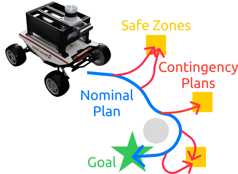
For safety, autonomous systems must be able to consider sudden changes and enact contingency plans appropriately. State-of-the-art methods currently find trajectories that balance between nominal and contingency behavior, or plan for a singular contingency plan; however, this does not guarantee that the resulting plan is safe for all time. To address this research gap, this paper presents Contingency-MPPI, a data-driven optimization-based strategy that embeds contingency planning inside a nominal planner. By learning to approximate the optimal contingency-constrained control sequence with adaptive importance sampling, the proposed method’s sampling efficiency is further improved with initializations from a lightweight path planner and trajectory optimizer. Finally, we present simulated and hardware experiments demonstrating our algorithm generating nominal and contingency plans in real time on a mobile robot.
Experiment Video Video will be added soon

keywords:

Contingency planning, model-predictive control, data-driven optimization, robotics

^†^†Distribution Statement A. Approved for public release: distribution unlimited^†^†\urlhttps://github.com/neu-autonomy/Contingency-MPPI

1 Introduction

Autonomous systems in real environments need to be able to handle sudden major changes in the operating conditions. For example, a car driving on the highway may need to swerve to safety if a collision occurs ahead, or a humanoid robot may need to grab hold of a railing if its foot slips on the stairs. Since there may be only a fraction of a second to recognize and respond to such events, this paper aims to develop an approach for always ensuring a contingency plan is available and can be immediately executed, if necessary.

A key challenge in this problem is to ensure a contingency plan always exists, without impacting the nominal plan too much. In standard approaches, where the nominal planner does not account for contingencies, the system could enter states from which no contingency plan exists; this may be tolerable if the failure event never occurs while the system is in one of those states but could lead to major safety failures in the worst case. [9683388] considered these backup plans by adding weighted terms to the cost function, which encourage staying out of these contingency-free areas, but does not have any guarantee. Alternatively, the methods of [alsterda2021contingency] and [9729171] explicitly plan alternative trajectories through a branching scheme and optimize both a nominal and set of contingency trajectories simultaneously. However, again, these methods must balance between the nominal trajectory cost and the tree of backup plans. [9729171, li2023marc, 10400882] all addressed risk-aware contingency planning with stochastic interactions with other agents; thus, these algorithms aim to minimize risk and cost over a tree of possible future scenarios, again only providing a balance between aggressive and safe behavior. [tordesillas2019faster] solved a contingency constrained problem by planning both an optimistic plan and a contingency plan that branches off to stay in known-free space. However, for more complicated safety requirements (e.g., a collection of safe regions that must remain reachable within a given time limit), the mixed integer programming problem proposed in that work becomes too expensive to solve in real time.

This leads to another important challenge: ensuring computational efficiency despite needing to generate both a nominal and a contingency plan from each state along the way. One approach would be to use exact reachability algorithms (e.g., 8263977; 9341499) to keep the planner out of contingency-free areas. However, computing the reachable sets is expensive, not strictly necessary, and would still require subsequently finding the contingency trajectories. Instead, this paper proposes to use an inexpensive contingency planner embedded inside the nominal planner. If the contingency planner finds a valid contingency plan, the nominal planner knows that state is acceptable, and the corresponding contingency plan is already available. Meanwhile, if the contingency planner fails to find a trajectory within a computation budget, the nominal planner can quickly (albeit conservatively) update its plans to avoid that state. To handle these discrete contingency events on top of generic nominal planning problems, our method, Contingency-MPPI, builds on model-predictive path integral (MPPI) control.

To summarize, this paper’s contributions include: (i) a planning algorithm that embeds contingency planning inside a nominal planner to ensure that a contingency plan exists from every state along the nominal plan, (ii) extensions of this planner using lightweight optimization problems to improve the sample-efficiency via better initial guesses, and (iii) demonstrations of the proposed method in simulated environments and on a mobile robot hardware platform to highlight the real-time implementation.

2 Problem Formulation

Refer to caption — Figure 1: At each step along the nominal plan, a contingency plan must exist to reach a safe state within a time horizon.

Denote a general nonlinear discrete-time system $\mathbf{x}_{t+1}=f(\mathbf{x}_{t},\mathbf{u}_{t})$ with state, $\mathbf{x}_{t}\in\mathbb{R}^{n_{x}}$ , and control, $\mathbf{u}_{t}\in\mathbb{R}^{n_{u}}$ at time $t$ . To indicate a trajectory, we use colon notation (e.g., $\mathbf{x}_{0:T}=\{\mathbf{x}_{0},\mathbf{x}_{1},\ldots,\mathbf{x}_{T}\}$ ) and $T$ -step dynamics $\mathbf{x}_{t+T}=f(\mathbf{x}_{t},\mathbf{u}_{0:T})$ . Additionally $\bm{U}\in\mathbb{R}^{n_{u}T}$ and $\bm{X}\in\mathbb{R}^{n_{x}T}$ indicate the state and control trajectory reshaped into a vector, and $\mathbf{\Sigma}\in\mathbb{R}^{n_{u}T\times n_{u}T}$ represents the covariance matrix of the reshaped control trajectory.

The contingency-constrained planning problem is to find a nominal trajectory, $\mathbf{u}_{0:T}$ , to minimize cost $J_{\text{nom}}$ , along with contingency trajectories $\{\mathbf{u}^{0}_{0:T_{c}},\ \allowbreak\ldots,\ \allowbreak\mathbf{u}^{T}_{0:T_{c}}\}$ that drive the system into a safe set, $\mathcal{S}$ , within $T_{c}$ steps, from each state along the nominal trajectory:


$\displaystyle\min_{\mathbf{u}_{0:T},\{\mathbf{u}^{0}_{0:T_{c}},\ldots,\mathbf{u}^{T}_{0:T_{c}}\}}$	$\displaystyle J_{\text{nom}}(\mathbf{x}_{0},\mathbf{u}_{0:T})$		(1a)
s.t.	$\displaystyle\mathbf{x}_{t+1}=f(\mathbf{x}_{t},\mathbf{u}_{t})$	$\displaystyle\forall{t\in[0,\ldots,T]}\,\,$	(1b)
	$\displaystyle\exists\tau\leq T_{c}\ \textrm{s.t.}\ f(\mathbf{x}_{i},\mathbf{u}^{i}_{0:\tau})\in\mathcal{S}$	$\displaystyle\forall{i\in[0,\ldots,T]}.$	(1c)

Other common costs/constraints (e.g., obstacle avoidance, control limits), can be added as desired.

3 Contingency-MPPI

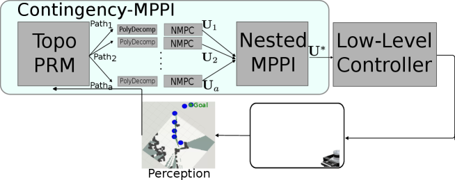
Ignoring the contingency constraint Eq. 1c, MPPI is a powerful method for solving Eq. 1 when the dynamics or costs are non-convex. This section shows how to extend MPPI to handle Eq. 1c as well, by nesting another sampling process into MPPI. First, we review the vanilla MPPI algorithm in Section 3.1, then describe our Nested-MPPI in Section 3.2. To increase sampling efficiency, a path-finding and trajectory optimization step (Section 3.3) is used to seed Nested-MPPI (LABEL:sec:backend) with ancillary controllers. This approach is summarized in Fig. 2.

3.1 Background: Model Predictive Path Integral Control

To summarize MPPI following asmar2023model, consider the entire control trajectory as a single input $\bm{V}\sim\mathcal{N}(\boldsymbol{U},\boldsymbol{\Sigma})$ , sampled from distribution $\mathbb{Q}$ with density

q(\boldsymbol{V})=((2\pi)^{n_{u}T}|\boldsymbol{\Sigma}|)^{-\frac{1}{2}}e^{-\frac{1}{2}(\boldsymbol{V}-\boldsymbol{U})^{T}\boldsymbol{\Sigma}^{-}1(\boldsymbol{V}-\boldsymbol{U})},

(2)

where $\bm{U},\bm{\Sigma}$ are the mean and covariance of $\mathbb{Q}$ . The objective of MPPI is to minimize the KL-divergence between this proposed distribution, $\mathbb{Q}$ , and an (unknown) optimal control distribution $\mathbb{Q}^{*}$ , defined with respect to a cost function of the form

\mathcal{J}(\boldsymbol{X},\boldsymbol{U})=\mathbb{E_{Q}}[\phi(\boldsymbol{X})+c(\boldsymbol{X})+\frac{\lambda}{2}\boldsymbol{U}^{T}\boldsymbol{\Sigma}^{-1}\boldsymbol{U}].

(3)

The optimal control distribution $\mathbb{Q}^{*}$ has density $q^{*}(\boldsymbol{V})=\frac{1}{\eta}(-\frac{1}{\lambda}S(\boldsymbol{V}))p(\boldsymbol{V})$ , based on a state-dependent cost, $S(\boldsymbol{V})=\phi(\boldsymbol{X})+c(\boldsymbol{X})$ and a nominal control distribution, $\mathbb{P}$ , with density

p(\boldsymbol{V})=((2\pi)^{n_{u}T}|\boldsymbol{\Sigma}|)^{-\frac{1}{2}}e^{-\frac{1}{2}(\boldsymbol{V}-\tilde{\boldsymbol{U}})^{T}\boldsymbol{\Sigma}^{-}1(\boldsymbol{V}-\tilde{\boldsymbol{U}})}.

(4)

Here, $\eta$ is a normalizing constant, $\lambda$ is the inverse temperature, and $\tilde{\boldsymbol{U}}$ is the base control, which is usually either zero or a nominal distribution from iterations of adaptive importance sampling. Then, to find the optimal control trajectory we can minimize the KL-divergence between $\mathbb{Q}$ and $\mathbb{Q}^{*}$ ,

\boldsymbol{U}^{*}=\arg\min_{\boldsymbol{U}}\mathbb{D}_{KL}(\mathbb{Q}^{*}||\mathbb{Q}).

(5)

Using adaptive importance sampling, the optimal control can be approximated by drawing $N$ samples from a distribution $\mathbb{Q}_{\hat{\boldsymbol{U}}}$ with proposed input $\hat{\boldsymbol{U}}$ ,

	$\displaystyle\boldsymbol{U}^{*}=\mathbb{E}_{\mathbb{Q}}[w(\boldsymbol{V})\boldsymbol{V}],$		(6)
	$\displaystyle w(\boldsymbol{V})=\frac{1}{\eta}e^{-\frac{1}{\lambda}(S(\boldsymbol{V})+\lambda(\hat{\boldsymbol{U}}-\tilde{\boldsymbol{U}})^{T}\Sigma^{-1}\boldsymbol{V})}$		(7)
	$\displaystyle\eta=\int e^{-\frac{1}{\lambda}(S(\boldsymbol{V})+\lambda(\hat{\boldsymbol{U}}-\tilde{\boldsymbol{U}})^{T}\Sigma^{-1}\boldsymbol{V})}d\boldsymbol{V}.\vspace{-1cm}$		(8)

(6) finds an (information-theoretic) optimal open-loop control sequence that can be implemented in a receding horizon by shifting one timestep ahead and re-running the algorithm. As in asmar2023model, we weigh the control cost by a factor $\gamma=\lambda(1-\alpha)$ and shift all sampled trajectory costs by the minimum sampled cost, for numerical stability.

3.1.1 Enforcing Hard Constraints in MPPI

While MPPI does not explicitly handle constraints, such as avoiding obstacles or the existence of a contingency plan, one can add terms to the objective with infinite cost when constraints are violated. For example, with a nominal cost $S_{\text{nom}}(\bm{V})$ and $N$ constraints, the augmented cost is $S(\boldsymbol{V})=S_{\text{nom}}(\bm{V})+\sum_{k=1}^{N}S_{\text{constraint}}^{k}(\bm{V})$ , where

S_{\text{constraint}}^{k}(\bm{V})=\cases{0},&\text{ifconstraintkissatisfied}\\ \infty,\text{o.w.}.

(9)

When the constraints are satisfied, the trajectory cost (and its weight in importance sampling) depends only on the nominal cost, such as minimum time or distance to the goal. If the constraints are not satisfied, the trajectory has infinite cost and receives zero weight in importance sampling. Thus, only trajectories meeting all constraints are considered, and their weights depend solely on the nominal cost. If no trajectory satisfies all constraints in an iteration, all samples get zero weight, and the mean control trajectory remains unchanged for the next MPPI iteration. However, if any trajectory met the constraints in the previous step, the executed control trajectory will still be safe

3.2 Nested-MPPI

{algorithm2e}

[H] \DontPrintSemicolon

Input: $\mathbf{x}_{0},\bm{U},[\bm{U}_{a}],\bm{\Sigma}$

Output: Nominal & contingency control sequences

Parameters: $K,T,L$ (nominal); $f,G,$ (system); $c,\phi,\lambda,\alpha$ (cost)

\BlankLine

$\bm{U}^{\prime}\leftarrow\bm{U}$ ; $\bm{\Sigma}^{\prime}\leftarrow\bm{\Sigma}$ \For(\tcp*[f]AIS loop) $l\leftarrow 0$ \KwTo $L-1$ \For $k\leftarrow 0$ \KwTo $K-1+\text{card}([\bm{U}_{a}])$ $\mathbf{x}_{k,0}\leftarrow\mathbf{x_{0}}$

$\bm{\mathcal{E}}_{k}\sim\mathcal{N}(0,\bm{\Sigma^{\prime}})$

\lIf

$k\leq K-1$ $\bm{U}=\bm{U}^{\prime}+\bm{\mathcal{E}}_{k}$ \tcpAncillary Control \lElse $\bm{U}=[\bm{U}_{a}]_{k-(K-1)}$ \For $i\leftarrow 0$ \KwTo $T-1$ $\mathbf{x}_{k,i+1}=\mathbf{x}_{k,i}+\left(f+G\left(\mathbf{u}\right)\right)\Delta t$ $\bm{U}_{\text{reach}_{k}},S_{\text{reach}}\leftarrow\text{FindContingencyPlan}(\bm{X}_{k})$ \lIf $S_{\text{reach}}=0$ $\bm{U}_{\text{contingency}}\leftarrow\bm{U}_{\text{reach}_{k}}$ $S_{k}\leftarrow S_{\text{reach}}+c(\bm{X})+\phi(\bm{X})+\lambda(1-\alpha)\bm{U}^{\prime T}\bm{\Sigma}^{-1}(\bm{\mathcal{E}}_{k}+\bm{U}^{\prime}-\bm{U})$ \lIf $l<L-1$ $\bm{U}^{\prime},\bm{\Sigma}^{\prime}\leftarrow\text{AIS}()$

\BlankLine

$\rho\leftarrow\min(\textbf{S})$ $\eta\leftarrow\sum_{k=1}^{K}\exp\left(-\frac{1}{\lambda}(S_{k}-\rho)\right)$

\For

$k\leftarrow 0$ \KwTo $K-1$ $\bm{U}\mathrel{+}=\frac{1}{\eta}\exp\left(-\frac{1}{\lambda}(S_{k}-\rho)\right)\left(\bm{\mathcal{E}}_{k}+\bm{U}^{\prime}-\bm{U}\right)$

\Return

$\bm{U},\bm{U}_{\text{contingency}}$ Nested-MPPI

{algorithm2e}

[H] \DontPrintSemicolon

Input: $\bm{X}$ : State sequence

Output: Contingency control sequence & score

Parameters: $K_{\text{c}},T_{\text{c}},L_{\text{c}},T_{\text{s}}$ (contingency); $f,G,m_{\text{elite}}$ (system/sampling); $\varepsilon,\lambda,\alpha$ (costs)

\BlankLine

$\bm{U}^{\prime}\leftarrow\bm{0}$

\For

$i\leftarrow 0$ \KwTo $T_{\text{s}}-1$ \For $l\leftarrow 0$ \KwTo $L_{\text{c}}-1$ $\mathbf{x}\leftarrow\mathbf{x}_{i}$ \For $k\leftarrow 0$ \KwTo $K_{\text{c}}-1$ \lIf $l=0$ $\bm{\mathcal{E}}_{k}\sim\text{U}(\bm{u}_{lb},\bm{u}_{ub})$ else $\bm{\mathcal{E}}_{k}\sim\mathcal{N}(0,\bm{\Sigma})$ \For $i\leftarrow 0$ \KwTo $T-1$ $\mathbf{x}_{k,i+1}=\mathbf{x}_{k,i}+(f+G(\mathbf{u}_{i}^{\prime}+\bm{\epsilon}_{i,k}^{\prime}))\Delta t$ $S_{k}\leftarrow\min_{\zeta\in\mathcal{S},\mathbf{x}\in\boldsymbol{X}^{s}}\|\mathbf{x}-\zeta\|$ \lIf $l>0$ $S_{k}\mathrel{+}=\lambda(1-\alpha)\bm{U}^{\prime T}\bm{\Sigma}^{-1}(\bm{\mathcal{E}}_{k}+\bm{U}^{\prime}-\bm{U})$ \lIf $l=0$ $\bm{U}_{\text}{best}\leftarrow\text{selectBest}(\bm{U},m_{\text}{elite},S)$ $\bm{U}^{\prime},\bm{\Sigma}^{\prime}\leftarrow\text{Mean}(\bm{U}_{\text}{best}),\text{Cov}(\bm{U}_{\text}{best})$

\lElseIf

$l<L_{\text{c}}-1$ $\bm{U}^{\prime},\bm{\Sigma}^{\prime}\leftarrow\text{AIS}()$ \lIf $\min(c_{i})<\varepsilon$ $S_{i,\text{reach}}\leftarrow 0$ else $S_{i,\text{reach}}\leftarrow\infty$

\Return

$\bm{U}^{\prime}_{0},\sum_{i=0}^{T_{\text{safe}}-1}S_{i,\text{reach}}$ $\text{FindContingencyPlan}$

This section introduces Nested-MPPI, which is summarized in Section 3.2. This algorithm is based on the MPPI in alsterda2021contingency and allows for ancillary controllers as proposed in trevisan2024biased. Our key innovation begins on Section 3.2, where a second level of MPPI executes in each state along each rollout of the nominal MPPI. This second level, described in Section 3.2, optimizes for a contingency plan (with a different cost function than the nominal plan) as a way of evaluating the reachability constraint, Eq. 1c.

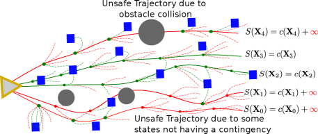
To both find contingency trajectories and evaluate whether the reachability constraint (1c) is satisfied for any control sequence, we first roll out each control sequence $\bm{U}_{i}$ by passing it through the zero-noise nonlinear dynamics model to get the state sequence $\boldsymbol{X}_{i}$ . Then, at each state $\mathbf{x}_{t}$ for $t=0,\dots,T_{s}-1$ , we run $L_{\text{c}}$ rounds of adaptive importance sampling MPPI with $N_{c}$ samples and $T_{c}$ timesteps starting at $\mathbf{x}_{t}$ to generate contingency state $[\bm{X}_{0}^{s},\dots,\bm{X}_{L\times N_{c}}^{s}]$ and control $[\bm{U}_{0}^{s},\dots,\bm{U}_{L\times N_{c}}^{s}]$ trajectories (lines 3.2-3.2 in Alg. 3.2). To encourage these contingency trajectories to reach safe states within $T_{c}$ timesteps, we use state-dependent cost

c_{\text}{contingency}(\boldsymbol{X}^{s})=\min_{\zeta\in\mathcal{S},\mathbf{x}\in\boldsymbol{X}^{s}}\|\mathbf{x}-\zeta\|.

(10)

Then, as seen in Figure 3, if any of the contingency trajectories successfully reaches a safe state within $T_{c}$ timesteps, we mark that state $\mathbf{x}_{t}$ along $\bm{X}_{i}$ as safe (green). If all states along $\bm{X}_{i}$ are marked as safe, then we mark $\bm{X}_{i}$ and its corresponding control $\bm{U}_{i}$ as safe; otherwise, we mark the trajectory as unsafe, and add $+\infty$ to its corresponding cost. In Section 3.2 Section 3.2, to initialize the proposed distribution for contingencies at each state, a number of sample control trajectories are drawn from a uniform distribution along control bounds $\mathbf{u}_{t,0:T_{c}}\sim U(\mathbf{u}_{\text{lb}},\mathbf{u}_{\text}{ub})$ , and the cross-entropy method is used on the best $m$ trajectories to determine an initial mean and covariance.

3.3 Improving the Sampling Efficiency of Nested-MPPI: Frontend

Although Section 3.2 considers all costs and constraints from Eq. 1, the sampling process can result in many or even all trajectories with infinite costs (if the sampling distribution is far from the optimal distribution), which leads to uninformed updates to the distribution. To remedy this, one may simply sample more $\boldsymbol{U}$ sequences; however, each additional sequence requires computing $S_{\text{reach}}$ , which requires an additional $T_{s}$ MPPI computations. Thus, rather than simply increasing the number of samples, we propose to approximate locally optimal $\boldsymbol{U}$ and consider them as a new sampling distribution(s) into Section 3.2, as described in LABEL:sec:backend. First, we find several different paths between the start and goal. For each path, we then perform a convex decomposition to find an under approximation of the safe space, and finally perform a nonlinear MPC to solve for a candidate control sequence.

3.3.1 Topo-PRM

To find several alternative paths through the workspace, we leverage Topo-PRM proposed in 9196996. As Topo-PRM finds a collection of topologically distinct paths through the environment, our planner can ”explore” the free-space and return multiple promising guiding paths. However as Topo-PRM does not consider safe zones, it may return paths that are not near safe zones, and thus no contingencies exist. Thus, we modify the algorithm to sample randomly from safe states $p$ fraction of the time to bias our roadmap to find paths that include safe states. To further bias the paths towards safe zones, denoting $V_{\text}{max}$ as the maximum speed of our vehicle in the creation of our workspace occupancy grid, we add pseudo-obstacles by marking occupied voxels that are farther than $r_{\text}{max}=V_{\text}{max}T_{s}\Delta t$ away from any given safe zone.

3.3.2 Nonlinear MPC

To transform each path into an ancillary control trajectory, we first find the point $E$ that is $r_{\text}{max}$ along the path, and then perform a convex decomposition using the approach from 7839930 of the free space along the path from our start point $S$ to $E$ . Next, we find $M$ knot points by discretizing $M-1$ points along the path from $S$ to $E$ . Denoting $A_{i}\mathbf{p}<b_{i}$ the polyhedral constraint in which point $p_{i}$ lies within, we solve the following nonlinear programming problem to recover a candidate ancillary control trajectory: