Constructive Observer Design for Visual Simultaneous Localisation and Mapping

Pieter van Goor
Department of Electrical, Energy and Materials Engineering
Australian National University
ACT, 2601, Australia
Pieter.vanGoor@anu.edu.au
&

Robert Mahony
Department of Electrical, Energy and Materials Engineering
Australian National University
ACT, 2601, Australia
Robert.Mahony@anu.edu.au
&

Tarek Hamel
I3S (University Côte d’Azur, CNRS, Sophia Antipolis)
and Insitut Universitaire de France
THamel@i3s.unice.fr
&

Jochen Trumpf
Department of Electrical, Energy and Materials Engineering
Australian National University
ACT, 2601, Australia
Jochen.Trumpf@anu.edu.au

Abstract

Visual Simultaneous Localisation and Mapping (VSLAM) is a well-known problem in robotics with a large range of applications. This paper presents a novel approach to VSLAM by lifting the observer design to a novel Lie group $\mathbf{VSLAM}_{n}(3)$ on which the system output is equivariant. The perspective gained from this analysis facilitates the design of a non-linear observer with almost semi-globally asymptotically stable error dynamics. Simulations are provided to illustrate the behaviour of the proposed observer and experiments on data gathered using a fixed-wing UAV flying outdoors demonstrate its performance.

1 Introduction

Refer to caption — Figure 1: The Disco Parrot UAV used to gather video data to test the proposed observer.

Simultaneous Localisation and Mapping (SLAM) has been an established problem in mobile robotics for at least the last 30 years [10]. Visual SLAM (VSLAM) refers to the special case where the only exteroceptive sensors available are cameras, and is frequently used to refer to the challenging situation where only a single monocular camera is available. The inherent non-linearity of the VSLAM problem remains challenging [8] and state-of-the-art solutions suffer from high computational complexity and poor scalability [10, 19]. Due to the low cost and low weight, as well as the ubiquity of single camera systems, the VSLAM problem remains an active research topic [10, 9].

Both the SLAM and VSLAM problems have recently attracted interest in the non-linear observer community, drawing from earlier work on attitude estimation [15, 5] and pose estimation [1, 23, 12]. Bonnabel et al. [2] exploited a novel Lie group to design an invariant Extended Kalman Filter for the SLAM problem. Parallel work by Mahony et al. [16] proposed the same group structure along with a novel quotient manifold structure for the state-space of the SLAM problem. Work by Zlotnik et al. [24] derives a geometrically motivated observer for the SLAM problem that includes estimation of bias in linear and angular velocity inputs. For the VSLAM problem, where only bearing measurements are available, Lourenco et al. [13, 14] proposed an observer with a globally exponentially stable error system using depths of landmarks as separate components of the observer. Bjorne et al. [4] use an attitude heading reference system (AHRS) to determine the orientation of the robot, and then solve the SLAM problem using a linear Kalman filter. A similar approach to VSLAM is undertaken by Le Bras et al. [6]. Hamel et al. [11] have also introduced a Riccati observer for the case where the orientation of the robot is known. Recent work by the authors [22] introduced a new symmetry structure specifically targeting the VSLAM problem but used an observer design that was a lifted version of that proposed in [11].

In this paper we present a novel non-linear equivariant observer for the VSLAM problem. The approach uses the SLAM manifold state-space proposed in [16] along with a novel symmetry Lie-group, $\mathbf{VSLAM}_{n}(3)$ , introduced by van Goor [22] but fully developed for the first time in this paper. We extend the results of [22] by providing compatible group actions on the state and output spaces and defining an intrinsic error that is globally defined. We propose a non-linear Lyapunov function expressed in the intrinsic error coordinates and use this to construct an observer for the visual SLAM problem posed on the symmetry group $\mathbf{VSLAM}_{n}(3)$ . This is in contrast to the majority of state-of-the-art algorithms which depend on local error coordinates and local linearisation [8]. (Although the recent IEKF results [7] exploit a global symmetry of the state-space the symmetry used is not compatible with visual bearings and the algorithm still depends on local linearisation.) In our proposed algorithm, separate constant gains for landmark bearing and depth estimates are used, making the design algebraically simple and leading to low-computational cost. We show that the error dynamics are almost semi-globally asymptotically stable (Def. A.1); that is, for any open neighbourhood of the error equilibrium, excluding a known exception set of measure zero, there exists a choice of gains such that this open set lies within the basin of attraction of the error equilibrium. As a result the algorithm is highly robust to measurement noise and also to data-association errors. Its low-computation and memory requirements make it ideally suited to embedded systems applications in consumer electronics.

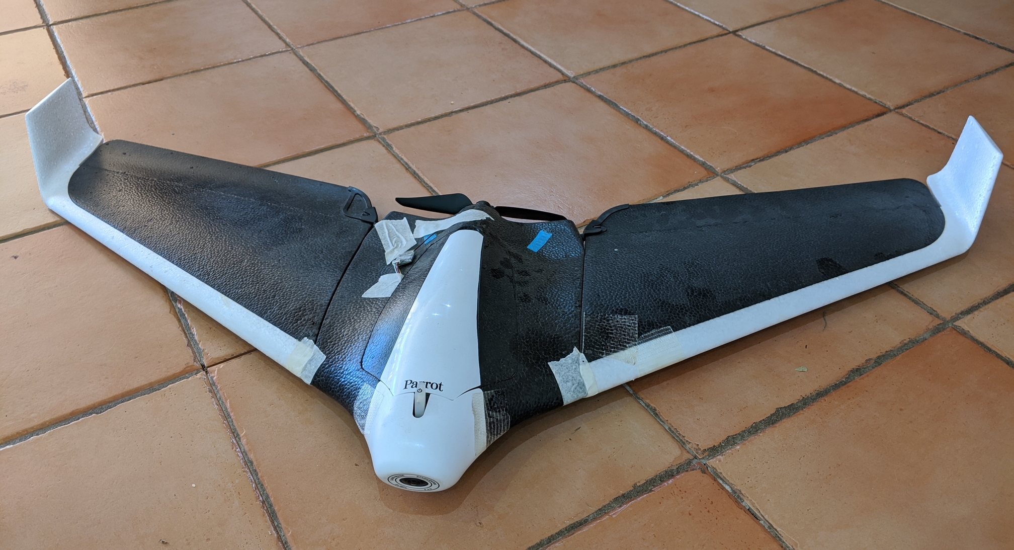
This paper consists of six sections alongside the introduction and conclusion. Section 2 introduces key notation and identities. In Section 3, we formulate the kinematics, state-space and output of the VSLAM system, and in Section 4 we introduce the Lie group $\mathbf{VSLAM}_{n}(3)$ and its actions on the state and output spaces. In Section 5 we derive a non-linear observer on the Lie group, and in Sections 6 and 7 we provide the results of a simulation and a real-world experiment carried out using a Disco Parrot UAV (Figure 1). The principal contribution of the paper is theoretical and the experimental sections support this by illustrating the properties of the algorithm and demonstrating that it functions on real-world data. We do not aspire to provide a comprehensive benchmark of performance against state-of-the-art SLAM systems in the present paper.

2 Preliminaries

2.1 Notation

The special orthogonal and special Euclidean matrix Lie groups are denoted $\mathbf{SO}(3)$ and $\mathbf{SE}(3)$ , respectively, with Lie algebras $\mathfrak{so}(3)$ and $\mathfrak{se}(3)$ . For any column vector $\Omega=(\Omega_{1},\Omega_{2},\Omega_{3})\in\mathbb{R}^{3}$ , the corresponding skew-symmetric matrix is denoted

\displaystyle\Omega^{\times}:=\left(\begin{matrix}0&-\Omega_{3}&\Omega_{2}\\ \Omega_{3}&0&-\Omega_{1}\\ -\Omega_{2}&\Omega_{1}&0\end{matrix}\right)\in\mathfrak{so}(3).

This matrix has the property that, for any $v\in\mathbb{R}^{3}$ , $\Omega^{\times}v=\Omega\times v$ where $\Omega\times v$ is the vector (cross) product between $\Omega$ and $v$ . For any unit vector $y\in\mathrm{S}^{2}\subset\mathbb{R}^{3}$ and any vector $v\in\mathbb{R}^{3}$ ,

\displaystyle y^{\times}y^{\times}v

\displaystyle=yy^{\top}v-v.

(1)

Consider a homogeneous matrix $P\in\mathbf{SE}(3)$ . The notation $R_{P}\in\mathbf{SO}(3)$ and $x_{P}\in\mathbb{R}^{3}$ is used to represent the rotation and translation components of $P$ , respectively; that is

\displaystyle P=\begin{pmatrix}R_{P}&x_{P}\\ 0&1\end{pmatrix}\in\mathbf{SE}(3).

Likewise, for a matrix $U\in\mathfrak{se}(3)$ , the notation $\Omega_{U}^{\times}\in\mathfrak{so}(3)$ , with $\Omega_{U}\in\mathbb{R}^{3}$ , and $V_{U}\in\mathbb{R}^{3}$ represent the angular and linear velocity components of $U$ , respectively; that is

\displaystyle U=\begin{pmatrix}\Omega_{U}^{\times}&V_{U}\\ 0&0\end{pmatrix}\in\mathfrak{se}(3).

3 Problem Formulation

3.1 VSLAM State Space

Fix an arbitrary reference frame $\{0\}$ . Let $P\in\mathbf{SE}(3)$ and $p_{i}\in\mathbb{R}^{3},i=1,...,n$ represent the robot pose and landmark coordinates, respectively, defined with respect to $\{0\}$ . The raw coordinates of the SLAM problem are written $(P,p_{1},...,p_{n})\in\mathbf{SE}(3)\times\mathbb{R}^{3}\times\cdots\times\mathbb{R}^{3}$ . The notation $(P,p_{i})\equiv(P,p_{1},...,p_{n})$ is used for simplicity in the sequel.

The physical measurements in a monocular VSLAM system are the bearings (3D directions) of landmarks perceived by the robot. We assume from now on that the observed landmarks and the robot are not collocated to ensure that the bearing measurements are well defined. Interestingly, this assumption has a substantive impact on the nature of the global symmetries that can be admitted. We make this assumption explicit, defining the total space $\mathcal{T}^{\circ}_{n}(3)$ of SLAM configurations considered to be

\mathcal{T}^{\circ}_{n}(3)=\big{\{}(P,p_{i})\in\mathbf{SE}(3)\times\mathbb{R}^{3}\times\cdots\times\mathbb{R}^{3}\ \vline\\ p_{i}\neq x_{P},i=1,...,n\big{\}}.

(2)

We assume that the trajectory of the robot remains in $\mathcal{T}^{\circ}_{n}(3)$ for all time.

Given two configurations $(P,p_{i}),(P^{\prime},p^{\prime}_{i})\in\mathcal{T}^{\circ}_{n}(3)$ , then $(P,p_{i})\simeq(P^{\prime},p^{\prime}_{i})$ if there exists $S\in\mathbf{SE}(3)$ such that $(P,p_{i})=(S^{-1}P^{\prime},R_{S}^{\top}(p^{\prime}_{i}-x_{S}))$ . That is, two sets of coordinates in the total space $\mathcal{T}^{\circ}_{n}(3)$ are considered equivalent when they are related by a rigid body transformation of the reference frame $\{0\}$ . It is straightforward to show the relation $\simeq$ is an equivalence relation on $\mathcal{T}^{\circ}_{n}(3)$ and

\displaystyle\lfloor P,p_{i}\rfloor:=\left\{(S^{-1}P,R_{S}^{\top}(p_{i}-x_{S}))\ \vline\ S\in\mathbf{SE}(3)\right\}.

is the associated equivalence class. The VSLAM manifold is the set

\displaystyle\mathcal{M}^{\circ}_{n}(3)=\left\{\lfloor P,p_{i}\rfloor\ |\ (P,p_{i})\in\mathcal{T}^{\circ}_{n}(3)\right\},

with quotient manifold structure. This is the open subset of the SLAM manifold $\mathcal{M}_{n}(3)$ considered in [16] without those equivalence classes where a landmark is co-located with the robot. Two configurations are equivalent on the SLAM manifold, $(P^{1},p_{i}^{1})\simeq(P^{2},p_{i}^{2})$ , if and only if the ego-centric coordinates of the landmarks are equal, $R_{P^{1}}^{\top}(p^{1}_{i}-x_{P^{1}})=R_{P^{2}}^{\top}(p^{2}_{i}-x_{P^{2}})$ for all $i$ .

3.2 VSLAM Kinematics

Assume that the robot is moving in a static environment. Define a velocity input vector space $\mathbb{V}=\mathfrak{se}(3)$ to contain the rigid-body velocity $U\in\mathfrak{se}(3)$ of the robot. The kinematics of the VSLAM system are given by the system function $f:\mathcal{T}^{\circ}_{n}(3)\times\mathbb{V}\to\mathrm{T}\mathcal{T}^{\circ}_{n}(3)$ ,

	$\displaystyle\frac{\mathrm{d}}{\mathrm{d}t}(P,p_{i})$	$\displaystyle=f((P,p_{i}),U),$
		$\displaystyle:=(PU,0).$		(3)

3.3 System Output

The camera measurements are modelled as elements of the sphere $\mathrm{S}^{2}$ . Each individual bearing is given by an output function $h^{i}:\mathcal{T}^{\circ}_{n}(3)\to\mathrm{S}^{2}$ ,

\displaystyle h^{i}(P,p_{i}):=\frac{R_{P}^{\top}(p_{i}-x_{P})}{\|p_{i}-x_{P}\|},

(4)

The output functions are well defined on $\mathcal{M}^{\circ}_{n}(3)$ since

$\displaystyle h^{i}(S^{-1}P,$	$\displaystyle R_{S}^{\top}(p_{i}-x_{S}))$
	$\displaystyle=\frac{(R_{S}^{\top}R_{P})^{\top}(R_{S}^{\top}(p_{i}-x_{S})-R_{S}^{\top}(x_{P}-x_{S}))}{\\|R_{S}^{\top}(p_{i}-x_{S})-R_{S}^{\top}(x_{P}-x_{S})\\|},$
	$\displaystyle=\frac{R_{P}^{\top}(p_{i}-x_{P})}{\\|p_{i}-x_{P}\\|}.$	(5)

The full output space of the VSLAM system is defined as a product of $n$ spheres,

\displaystyle\mathcal{N}^{n}(3):=\mathrm{S}^{2}\times\cdots\times\mathrm{S}^{2},

with a combined output function $h:\mathcal{T}_{n}(3)^{\circ}\to\mathcal{N}^{n}(3)$

\displaystyle h(P,p_{i}):=\left(\frac{R_{P}^{\top}(p_{1}-x_{P})}{\|p_{1}-x_{P}\|},\ldots,\frac{R_{P}^{\top}(p_{n}-x_{P})}{\|p_{n}-x_{P}\|}\right).

(6)

4 Symmetry of the VSLAM Problem

4.1 Symmetry of the Total Space $\mathcal{T}^{\circ}_{n}(3)$

Define a Lie group

\displaystyle\mathbf{VSLAM}_{n}(3)=SE(3)\times(\mathbf{SO}(3)\times\mathbf{MR}(1))^{n},

with product Lie group structure, where $\mathbf{MR}(1)$ is the multiplicative real group of positive real numbers. This Lie group was first proposed in van Goor et al. [22]. The associated Lie algebra is denoted $\mathfrak{vslam}_{n}(3)$ . We write elements of $\mathbf{VSLAM}_{n}(3)$ as $(A,(Q,a)_{i})\equiv(A,(Q,a)_{1},...,(Q,a)_{n})\in\mathbf{VSLAM}_{n}(3)$ .

Lemma 4.1.

The mapping $\Upsilon:\mathbf{VSLAM}_{n}(3)\times\mathcal{T}^{\circ}_{n}(3)\to\mathcal{T}^{\circ}_{n}(3)$ defined by

\Upsilon((A,(Q,a)_{i}),(P,p_{i})):=(PA,a_{i}^{-1}R_{PA}Q_{i}^{\top}R_{P}^{\top}(p_{i}-x_{P})+x_{PA}),

(7)

is a right group action of $\mathbf{VSLAM}_{n}(3)$ on $\mathcal{T}^{\circ}_{n}(3)$ .

Proof.

Trivially, $\Upsilon((I_{4},(I_{3},1)),(P,p_{i}))=(P,p_{i})$ for any $(P,p_{i})\in\mathcal{T}^{\circ}_{n}(3)$ . Let $(A_{1},(Q_{1},a_{1})_{i}),(A_{2},(Q_{2},a_{2})_{i})\in\mathbf{VSLAM}_{n}(3)$ and $(P,p_{i})\in\mathcal{T}^{\circ}_{n}(3)$ be arbitrary. Then

	$\displaystyle\Upsilon($	$\displaystyle(A_{1},(Q_{1},a_{1})_{i}),\Upsilon((A_{2},(Q_{2},a_{2})_{i}),(P,p_{i})))$
		$\displaystyle=(PA_{2}A_{1},(a_{1}^{-1}a_{2}^{-1}R_{PA_{2}A_{1}}Q_{1}^{\top}$
		$\displaystyle\hskip 28.45274ptQ_{2}^{\top}R_{P}^{\top}(p-x_{P}))+x_{PA_{2}A_{1}})_{i}),$
		$\displaystyle=\Upsilon((A_{2}A_{1},(Q_{2}Q_{1},a_{2}a_{1})_{i}),(P,p_{i})),$
		$\displaystyle=\Upsilon((A_{2},(Q_{2},a_{2})_{i})\cdot(A_{1},(Q_{1},a_{1})_{i}),(P,p_{i})).$

∎

4.2 Symmetry of the Output Space

There is an action $\rho$ of the $\mathbf{VSLAM}_{n}(3)$ group on the output space such that the measurement function $h$ defined in (6) is equivariant with respect to $\Upsilon$ and $\rho$ . The following lemmas define this action $\rho$ and show the equivariance of $h$ for the proposed $\mathbf{VSLAM}_{n}(3)$ geometry. The authors know of no output action that makes bearing outputs equivariant with respect to prior geometries proposed for SLAM [2, 16].

Proposition 4.2.

The mapping $\rho:\mathbf{VSLAM}_{n}(3)\times\mathcal{N}^{n}(3)\to\mathcal{N}^{n}(3)$ defined by

\displaystyle\rho((A,

\displaystyle(Q,a)_{i}),y_{i})=Q_{i}^{\top}y_{i},

(8)

is a right group action of $\mathbf{VSLAM}_{n}(3)$ on $\mathcal{N}^{n}(3)$ .

Proof.

The proof is straightforward. ∎

Lemma 4.3.

The output $h:\mathcal{T}^{\circ}_{n}(3)\to\mathcal{N}(3)$ (6) is equivariant with respect to actions $\Upsilon$ (7) and $\rho$ (8). That is, for any $X\in\mathbf{VSLAM}_{n}(3)$ and any $\xi\in\mathcal{T}^{\circ}_{n}(3)$ ,

\displaystyle h(\Upsilon(X,\xi))=\rho(X,h(\xi)).

Proof.

Let $X=(A,(Q,a)_{i})$ and $\xi=(P,p_{i})$ be arbitrary. Then

	$\displaystyle h(\Upsilon(X,\xi))$
	$\displaystyle=h\left(PA,a_{i}^{-1}R_{PA}Q_{i}^{\top}R_{P}^{\top}(p_{i}-x_{P})+x_{PA}\right),$
	$\displaystyle=\frac{R_{PA}^{\top}(a_{i}^{-1}R_{PA}Q_{i}^{\top}R_{P}^{\top}(p_{i}-x_{P})+x_{PA}-x_{PA})}{\\|a_{i}^{-1}R_{PA}Q_{i}^{\top}R_{P}^{\top}(p_{i}-x_{P})+x_{PA}-x_{PA}\\|},$
	$\displaystyle=\frac{Q_{i}^{\top}R_{P}^{\top}(p_{i}-x_{P})}{\\|p_{i}-x_{P}\\|},$
	$\displaystyle=\rho(X,h(\xi)).$

∎

4.3 Lift of the VSLAM Kinematics

In order to consider the system on the $\mathbf{VSLAM}_{n}(3)$ group, the kinematics from the total space must be lifted onto the group. A lift is a map $\Lambda:\mathcal{T}^{\circ}_{n}(3)\times\mathbb{V}\to\mathfrak{vslam}_{n}(3)$ such that

\displaystyle\mathrm{D}\Upsilon_{(P,p_{i})}(\mathrm{id})\left[\Lambda((P,p_{i}),U)\right]=f((P,p_{i}),U)

(9)

where $f((P,p_{i}),U)$ is given by (3).

Lemma 4.4.

The function $\Lambda:\mathcal{T}^{\circ}_{n}(3)\times\mathbb{V}\to\mathfrak{vslam}_{n}(3)$ , defined by

\displaystyle\Lambda((P,p_{i}),U):=(U,(\Lambda_{Q}(U,R_{P}^{\top}(p_{i}-x_{P})),\Lambda_{a}(U,R_{P}^{\top}(p_{i}-x_{P})))),

(10)

where $\Lambda_{Q}:\mathfrak{se}(3)\times(\mathbb{R}^{3}\setminus\{0\})\to\mathfrak{so}(3)$ is given by

\Lambda_{Q}\left(U,q\right):=\left(\Omega_{U}+\frac{q\times V_{U}}{|q|^{2}}\right)^{\times},

and $\Lambda_{a}:\mathfrak{se}(3)\times(\mathbb{R}^{3}\setminus\{0\})\to\mathfrak{mr}(1)$ is given by

\displaystyle\Lambda_{a}\left(U,q\right):=\frac{q^{\top}V_{U}}{|q|^{2}},

is a lift in the sense of (9) of the kinematics (3) onto $\mathfrak{vslam}_{n}(3)$ with respect to the group action (7).

Proof.

Given $(P,p_{i})\in\mathcal{T}^{\circ}_{n}(3)$ , let $q_{i}:=R_{P}^{\top}(p_{i}-x_{P})$ , $W^{\times}_{i}:=\Lambda_{Q}(U,q_{i})$ , and $w_{i}:=\Lambda_{a}(U,q_{i})$ . Then

$\displaystyle\mathrm{D}\Upsilon_{(P,p_{i})}(\mathrm{id})$	$\displaystyle\left[\Lambda((P,p_{i}),U)\right]$
	$\displaystyle=\mathrm{D}\Upsilon_{(P,p_{i})}(\mathrm{id})\left[(U,(W^{\times}_{i},w_{i}))\right]$
	$\displaystyle=\left(PU,v_{i}\right)$	(11)

where $v_{i}$ is

\displaystyle v_{i}=\left.\frac{\mathrm{d}}{\mathrm{d}s}\right|_{s=0}\left[(1+sw_{i})^{-1}R_{P(I_{4}+sU)}(I_{3}+sW_{i}^{\times})^{\top}q_{i}+x_{P(I_{4}+sU)}\right],

using group index notation. Computing this derivative and evaluating at $s=0$ one obtains

$\displaystyle v_{i}$	$\displaystyle=-w_{i}R_{P}q_{i}+R_{P}\Omega_{U}^{\times}q_{i}+R_{P}(W_{i}^{\times})^{\top}q_{i}+R_{P}V_{U},$
	$\displaystyle=-\frac{q_{i}^{\top}V_{U}}{\|q_{i}\|^{2}}R_{P}q_{i}+R_{P}\Omega_{U}^{\times}q_{i}+R_{P}V_{U}$
	$\displaystyle\hskip 56.9055pt-R_{P}\left(\Omega_{U}+\frac{q_{i}\times V_{U}}{\|q_{i}\|^{2}}\right)^{\times}q_{i},$	(12)
	$\displaystyle=-R_{P}\frac{q_{i}q_{i}^{\top}}{\|q_{i}\|^{2}}V_{U}+R_{P}V_{U}+R_{P}\frac{q_{i}q_{i}^{\top}}{\|q_{i}\|^{2}}V_{U}-R_{P}V_{U},$	(13)
	$\displaystyle=0,$

where (12) follows from substituting for $w_{i}$ and $W_{i}$ with the full expressions for $\Lambda_{a}$ and $\Lambda_{Q}$ , and (13) follows from cancelling the $\Omega_{U}$ term and using the relationship (1) as well as rearranging the first term. The result follows from substituting directly into (11) and recalling (3). ∎

5 Observer Design

5.1 Lifted System Kinematics

Let $\xi=(P,p_{i})\in\mathcal{T}^{\circ}_{n}(3)$ denote the true state of the VSLAM system. The kinematics of $\xi$ of the VSLAM system are given by (3). Choose an arbitrary origin configuration $\xi^{\circ}=(P^{\circ},p^{\circ}_{i})\in\mathcal{T}^{\circ}_{n}(3)$ . The lifted system is (Lemma 4.4)

\displaystyle\frac{\mathrm{d}}{\mathrm{d}t}X

\displaystyle=X\Lambda(\Upsilon(X,\xi^{\circ}),U),

(14)

for $X=(A,(Q,a)_{i})\in\mathbf{VSLAM}_{n}(3)$ . If $\Upsilon(X(0),\xi^{\circ})=\xi(0)$ then trajectories of the lifted system kinematics project to trajectories of the VSLAM kinematics (3) [17]. That is, recalling (7)

	$\displaystyle(P(t),p_{i}(t))$	$\displaystyle=\Upsilon(X(t),\xi^{\circ}),$
		$\displaystyle=(P^{\circ}A,a_{i}^{-1}R_{P^{\circ}A}Q_{i}^{\top}R_{P^{\circ}}^{\top}(p^{\circ}_{i}-x_{P^{\circ}})+x_{P^{\circ}A})$

for all $t\geq 0$ , where we have dropped the time dependence of $A$ , $Q_{i}$ and $a_{i}$ from the notation to improve readability.

5.2 Landmark Observer

The following theorem proposes an observer $\hat{X}\in\mathbf{VSLAM}_{n}(3)$ and provides innovation terms for the components of the observer $\hat{X}$ corresponding to each of the landmarks.

Theorem 5.1.

Fix an arbitrary origin configuration $\xi^{\circ}=(P^{\circ},p^{\circ}_{i})\in\mathcal{T}^{\circ}_{n}(3)$ . Let $X=(A,(Q,a)_{i})$ be a trajectory of the lifted system (14) associated with a trajectory $\xi=(P,p_{i})$ of the true system satisfying (3) for measured input signal $U=(\Omega_{U}^{\times},V_{U})$ . Let $y_{i}:=h^{i}(\xi)$ (4) denote the output. Assume that $|U|$ is bounded, and that there exist $0<\underline{r}<\overline{r}\in\mathbb{R}$ such that

\underline{r}\leq||p_{i}-x_{P}||\leq\overline{r}

for all time. For each $i$ , assume that $y_{i}^{\times}y_{i}^{\times}V_{U}$ is persistently exciting, in the sense that there exist $T>0$ and $\mu>0$ such that

\displaystyle\frac{1}{T}\int_{t}^{t+T}\|y_{i}^{\times}y_{i}^{\times}V_{U}\|\mathrm{d}\tau\geq\mu,

(15)

for all $t>0$ .

The observer state is $\hat{X}=(\hat{A},(\hat{Q},\hat{a})_{i})\in\mathbf{VSLAM}_{n}(3)$ , with kinematics given by

	$\displaystyle\frac{\mathrm{d}}{\mathrm{d}t}\hat{X}$	$\displaystyle:=\hat{X}\Lambda(\Upsilon(\hat{X},\xi^{\circ}),U)-\Delta_{\hat{X}}\hat{X},$
	$\displaystyle\hat{X}(0)$	$\displaystyle=\mathrm{id},$		(16)

where $\Lambda$ is the lift defined by (10) and $\Delta_{\hat{X}}=(\Delta,(\Gamma,\gamma)_{i})\in\mathfrak{vslam}_{n}(3)$ is the innovation defined below. The state estimate is given by $\hat{\xi}=(\hat{P},\hat{p}_{i})=\Upsilon(\hat{X},\xi^{\circ})$ (7).

Let $y^{\circ}_{i}:=h(\xi^{\circ})$ denote the origin output, and let $\delta_{i}$ denote the output error, defined as

\displaystyle\delta_{i}

\displaystyle=\rho(\hat{X}^{-1},y_{i})=\rho(X\hat{X}^{-1},y^{\circ}_{i}).

Define the true range $r_{i}=\|{p}_{i}-x_{{P}}\|$ and estimated range $\hat{r}_{i}=\|\hat{p}_{i}-x_{\hat{P}}\|$ for each $i$ . The range error is

\displaystyle\tilde{r}_{i}=\frac{\hat{r}_{i}}{r_{i}},

(17)

for each $i$ . For $k_{0}>0$ a positive gain let $\epsilon=\min(k_{0},\frac{1}{2})\underline{r}$ . Define the twice differentiable barrier function $\beta^{\epsilon}_{\underline{r}}:(\epsilon,\infty)\to[0,\infty)$ to be

\displaystyle\beta^{\epsilon}_{\underline{r}}(\hat{r}_{i})

\displaystyle:=\begin{cases}\frac{(\hat{r}_{i}-\underline{r})^{2}}{(\underline{r}-\epsilon)^{2}(\hat{r}_{i}-\epsilon)},&\epsilon<\hat{r}_{i}<\underline{r}\\ 0,&\hat{r}_{i}\geq\underline{r}\end{cases}.

(18)

The landmark innovation terms $\Gamma_{i}$ and $\gamma_{i}$ for $\Delta_{\hat{X}}$ are defined to be

$\displaystyle\Gamma_{i}$	$\displaystyle:=\left(\frac{\delta_{i}^{\top}\hat{Q}_{i}V_{U}}{2\hat{r}_{i}}-\frac{(\delta_{i}+y^{\circ}_{i})^{\top}}{\hat{r}_{i}(1+\delta_{i}^{\top}y^{\circ}_{i})}\hat{Q}_{i}V_{U}-k_{i}\right)(\delta_{i}^{\times}y^{\circ}_{i})^{\times},$
$\displaystyle\gamma_{i}$	$\displaystyle:=\frac{\alpha_{i}}{\hat{r}_{i}^{2}}\left(\frac{1-\delta_{i}^{\top}y^{\circ}_{i}}{2(1+\delta_{i}^{\top}y^{\circ}_{i})}\delta_{i}^{\top}\hat{Q}_{i}V_{U}-\frac{{y^{\circ}_{i}}^{\top}\Pi_{\delta_{i}}\hat{Q}_{i}V_{U}}{(1+\delta_{i}^{\top}y^{\circ}_{i})^{2}}\right)$
	$\displaystyle\quad+\frac{1}{\hat{r}_{i}}(y^{\circ}_{i}-\delta_{i})^{\top}\hat{Q}_{i}V_{U}+\frac{\alpha_{i}}{\hat{r}_{i}}\beta^{\epsilon}_{\underline{r}}(\hat{r}_{i}),$	(19)

where $k_{i}$ and $\alpha_{i}$ are constant positive scalars. The robot pose innovation $\Delta\in\mathbf{SE}(3)$ can be chosen to be any continuous function of the observer state and measurements (cf. §5.3).

Then (5.1) defines an almost semi-globally asymptotically stabilising (Def. A.1) innovation for the error dynamics for $\delta_{i},\tilde{r}_{i}$ around the equilibrium $(y^{\circ}_{i},1)$ with exception set

\displaystyle\chi=\{(\delta,\tilde{r})_{i}\in(\mathrm{S}^{2}\times\mathbb{R}_{+})^{n}\;|\;\delta_{i}

\displaystyle=-y^{\circ}_{i}\text{ for some }i\in[1,\ldots,n]\}.

(20)

Moreover, as $(\delta_{i},\tilde{r}_{i})\to(y^{\circ}_{i},1)$ , the estimated state $\hat{\xi}\to\xi$ converges to the true state up to the SLAM manifold equivalence.

Proof.

Let $K$ be a compact set in the complement of $\chi$ (20). Assume $(\delta_{i}(0),\tilde{r}_{i}(0))\in K$ and choose $k_{0}=\frac{1}{2}\min(\tilde{r}_{i}(0))>0$ . Then

	$\displaystyle\tilde{r}_{i}(0)$	$\displaystyle\geq k_{0},$
	$\displaystyle\hat{r}_{i}(0)$	$\displaystyle\geq k_{0}r_{i}(0)\geq k_{0}\underline{r}>0,$

for each $i$ . Thus $\hat{r}_{i}(0)>\epsilon>0$ for every $i$ by definition of $\epsilon$ . By continuity of the solutions there exist $T_{i}>0$ such that $\hat{r}_{i}(t)>\epsilon$ , and hence $\beta^{\epsilon}_{\underline{r}}(\hat{r}_{i})$ is well-defined, for $t\in[0,T_{i})$ . We will show later that $T_{i}$ can be chosen arbitrarily large and $\hat{r}_{i}(t)>\epsilon$ holds for all time.

For each $i$ , define the storage function

	$\displaystyle l_{i}(\delta_{i},\tilde{r}_{i};r_{i})$	$\displaystyle:=\frac{r_{i}}{2}\frac{\\|{y^{\circ}_{i}}-\delta_{i}\\|^{2}}{2-\\|{y^{\circ}_{i}}-\delta_{i}\\|^{2}}+\frac{r_{i}^{2}}{2\alpha_{i}}(1-\tilde{r}_{i})^{2}$
		$\displaystyle=\frac{r_{i}}{2}\frac{1-{y^{\circ}}_{i}^{\top}\delta_{i}}{1+{y^{\circ}}_{i}^{\top}\delta_{i}}+\frac{1}{2\alpha_{i}}(r_{i}-\hat{r}_{i})^{2}.$		(21)

in the variables $(\delta_{i},\tilde{r}_{i})$ where the second line follows from $\|\delta_{i}\|=\|y^{\circ}_{i}\|=1$ and substituting for $\tilde{r}_{i}$ . Note that $l_{i}$ depends on the time varying range $r_{i}$ as a parameter. By assumption, $r_{i}\geq\underline{r}>0$ and the storage functions $l_{i}$ are positive definite. Similarly, $\delta_{i}(0)\not=-y^{\circ}_{i}$ for all $i$ and $l_{i}$ is well-defined and finite at $t=0$ . By continuity of solutions there exist times $T^{\prime}_{i}>0$ such that the $l_{i}(t)$ remain well defined on the time interval $[0,T^{\prime}_{i})$ . Note that $T^{\prime}_{i}\leq T_{i}$ for each $i$ , as $l_{i}$ depends on $\hat{r}_{i}$ . We will show later that $l_{i}(t)$ are defined for all time.

By definition, $r_{i}=a_{i}^{-1}r^{\circ}_{i}$ , and $\hat{r}_{i}=\hat{a}_{i}^{-1}r^{\circ}_{i}$ . Differentiating these with respect to time yields

$\displaystyle\dot{r}_{i}$	$\displaystyle=-V_{U}^{\top}y_{i},$
$\displaystyle\dot{\hat{r}}_{i}$	$\displaystyle=-V_{U}^{\top}\hat{y}_{i}+\hat{r}_{i}\gamma_{i},$
	$\displaystyle=-V_{U}^{\top}y_{i}+\alpha_{i}\beta^{\epsilon}_{\underline{r}}(\hat{r}_{i})$	(22)
	$\displaystyle\quad+\frac{\alpha_{i}}{\hat{r}_{i}}\left(\frac{1-\delta_{i}^{\top}y^{\circ}_{i}}{2(1+\delta_{i}^{\top}y^{\circ}_{i})}\delta_{i}^{\top}\hat{Q}_{i}V_{U}-\frac{{y^{\circ}_{i}}^{\top}\Pi_{\delta_{i}}\hat{Q}_{i}V_{U}}{(1+\delta_{i}^{\top}y^{\circ}_{i})^{2}}\right),$

where $\hat{y}_{i}=h^{i}(\hat{\xi})$ is the estimated measurement. Since $\beta^{\epsilon}_{\underline{r}}$ (18) is a barrier function ensuring that $\hat{r}_{i}(t)>\epsilon$ , ( $\beta^{\epsilon}_{\underline{r}}(\hat{r}_{i})\to\infty$ as $\hat{r}_{i}\searrow\epsilon$ ,) it follows that the remaining terms in (22) are bounded and $\hat{r}_{i}$ is well defined $\forall t\in[0,T_{i})$ .

Differentiating the output error $\delta_{i}$ yields

	$\displaystyle\dot{\delta}_{i}$	$\displaystyle=\frac{\mathrm{d}}{\mathrm{d}t}\rho(X\hat{X}^{-1},y^{\circ})_{i}=\frac{\mathrm{d}}{\mathrm{d}t}\hat{Q}_{i}Q_{i}^{\top}y^{\circ}_{i},$
		$\displaystyle=\left(\hat{Q}_{i}\Lambda_{Q}(U,R_{\hat{P}}^{\top}(\hat{p}_{i}-x_{\hat{P}}))-\Gamma_{i}\hat{Q}_{i}\right)Q_{i}^{\top}y^{\circ}_{i}$
		$\displaystyle\hskip 28.45274pt-\hat{Q}_{i}\Lambda_{Q}(U,R_{P}^{\top}(p_{i}-x_{P}))Q_{i}^{\top}y^{\circ}_{i}.$

Observe that $R_{\hat{P}}^{\top}(\hat{p}_{i}-x_{\hat{P}})=\hat{r}_{i}\hat{y}_{i}$ and $R_{P}^{\top}(p_{i}-x_{P})=r_{i}y_{i}$ . Using this, the derivative of $\delta_{i}$ is simplified to

$\displaystyle\dot{\delta}_{i}$	$\displaystyle=\operatorname{Ad}_{\hat{Q}_{i}}\left(\Lambda_{Q}(U,\hat{r}_{i}\hat{y}_{i})-\Lambda_{Q}(U,r_{i}y_{i})\right)\delta_{i}-\Gamma_{i}\delta_{i},$
	$\displaystyle=\operatorname{Ad}_{\hat{Q}_{i}}\left(\frac{\hat{y}_{i}\times V_{U}}{\hat{r}_{i}}-\frac{y_{i}\times V_{U}}{r_{i}}\right)^{\times}\delta_{i}-\Gamma_{i}\delta_{i},$
	$\displaystyle=\left(\frac{{y^{\circ}_{i}}^{\times}\hat{Q}_{i}V_{U}}{\hat{r}_{i}}-\frac{\delta_{i}^{\times}\hat{Q}_{i}V_{U}}{r_{i}}\right)^{\times}\delta_{i}-\Gamma_{i}\delta_{i},$	(23)

where the last step is obtained by using various identities involving the skew symmetric operator.

Recalling (21) and using identities involving the skew symmetric operator and projector, the derivative of ${y^{\circ}}_{i}^{\top}\delta_{i}$ is

	$\displaystyle\frac{\mathrm{d}}{\mathrm{d}t}{y^{\circ}}_{i}^{\top}\delta_{i}={y^{\circ}}_{i}^{\top}\dot{\delta}_{i},$
	$\displaystyle=-\hat{r}_{i}^{-1}\delta_{i}^{\top}\Pi_{y^{\circ}_{i}}\hat{Q}_{i}V_{U}-r_{i}^{-1}{y^{\circ}}_{i}^{\top}\Pi_{\delta_{i}}\hat{Q}_{i}V_{U}$
	$\displaystyle\quad-\left(\frac{\delta_{i}^{\top}\hat{Q}_{i}V_{U}}{2\hat{r}_{i}}-\frac{(\delta_{i}+y^{\circ}_{i})^{\top}\hat{Q}_{i}V_{U}}{\hat{r}_{i}(1+\delta_{i}^{\top}y^{\circ}_{i})}-k_{i}\right){y^{\circ}_{i}}^{\top}(\delta_{i}^{\times}y^{\circ}_{i})^{\times}\delta_{i},$
	$\displaystyle=(\hat{r}_{i}^{-1}-r_{i}^{-1}){y^{\circ}}_{i}^{\top}\Pi_{\delta_{i}}\hat{Q}_{i}V_{U}$
	$\displaystyle\quad-\left(\frac{\delta_{i}^{\top}\hat{Q}_{i}V_{U}}{2\hat{r}_{i}}-k_{i}\right)(1-(\delta_{i}^{\top}y^{\circ}_{i})^{2}),$
	$\displaystyle=\frac{r_{i}-\hat{r}_{i}}{r_{i}\hat{r}_{i}}{y^{\circ}}_{i}^{\top}\Pi_{\delta_{i}}\hat{Q}_{i}V_{U}-\left(\frac{\delta_{i}^{\top}\hat{Q}_{i}V_{U}}{2\hat{r}_{i}}-k_{i}\right)(1-(\delta_{i}^{\top}y^{\circ}_{i})^{2}).$

The derivative of $l_{i}$ may now be computed on the time interval $[0,T^{\prime}_{i})$ as follows:

$\displaystyle\dot{l}_{i}$	$\displaystyle=\frac{\dot{r}_{i}}{2}\frac{1-{y^{\circ}}_{i}^{\top}\delta_{i}}{1+{y^{\circ}}_{i}^{\top}\delta_{i}}+\frac{r_{i}}{2}\frac{-2{y^{\circ}}_{i}^{\top}\dot{\delta}_{i}}{(1+{y^{\circ}}_{i}^{\top}\delta_{i})^{2}}$
	$\displaystyle\quad+\frac{1}{\alpha_{i}}(r_{i}-\hat{r}_{i})(\dot{r}_{i}-\dot{\hat{r}}_{i}),$
	$\displaystyle=\frac{-y_{i}^{\top}V_{U}}{2}\frac{1-{y^{\circ}}_{i}^{\top}\delta_{i}}{1+{y^{\circ}}_{i}^{\top}\delta_{i}}-\frac{r_{i}-\hat{r}_{i}}{\hat{r}_{i}}\frac{{y^{\circ}}_{i}^{\top}\Pi_{\delta_{i}}\hat{Q}_{i}V_{U}}{(1+{y^{\circ}}_{i}^{\top}\delta_{i})^{2}}$
	$\displaystyle\quad+\frac{r_{i}\delta_{i}^{\top}\hat{Q}_{i}V_{U}}{2\hat{r}_{i}}\frac{1-{y^{\circ}_{i}}^{\top}\delta_{i}}{1+{y^{\circ}_{i}}^{\top}\delta_{i}}-k_{i}\frac{1-{y^{\circ}_{i}}^{\top}\delta_{i}}{1+{y^{\circ}_{i}}^{\top}\delta_{i}}$
	$\displaystyle\quad+\frac{\hat{r}_{i}-r_{i}}{\hat{r}_{i}}\left(\frac{1-\delta_{i}^{\top}y^{\circ}_{i}}{2(1+\delta_{i}^{\top}y^{\circ}_{i})}\delta_{i}^{\top}\hat{Q}_{i}V_{U}-\frac{{y^{\circ}_{i}}^{\top}\Pi_{\delta_{i}}\hat{Q}_{i}V_{U}}{(1+\delta_{i}^{\top}y^{\circ}_{i})^{2}}\right)$
	$\displaystyle\quad+(\hat{r}_{i}-r_{i})\beta^{\epsilon}_{\underline{r}}(\hat{r}_{i}),$
	$\displaystyle=-k_{i}\frac{1-{y^{\circ}_{i}}^{\top}\delta_{i}}{1+{y^{\circ}_{i}}^{\top}\delta_{i}}+(\hat{r}_{i}-r_{i})\beta^{\epsilon}_{\underline{r}}(\hat{r}_{i}).$	(24)

The second term is negative semi-definite, since it is zero when $\hat{r}_{i}\geq\underline{r}$ (18), and otherwise $\hat{r}_{i}<\underline{r}\leq r_{i}$ and $\hat{r}_{i}-r_{i}\leq 0$ . It follows that $\dot{l}_{i}(t)\leq 0$ , and $l_{i}(t)\leq l_{i}(0)$ for all $t\in[0,T^{\prime}_{i})$ .

We show by contradiction that $T^{\prime}_{i}$ can be chosen arbitrarily large. Assume that there is an $i$ and maximum value $T^{\prime}_{i}$ for which $l_{i}(t)$ is well defined on $[0,T^{\prime}_{i})$ . Since $l_{i}(t)\leq l_{i}(0)$ on $[0,T^{\prime}_{i})$ and the solution of (24) is absolutely continuous then the limit $l_{i}(T^{\prime}_{i})=\lim_{t\rightarrow T^{\prime}_{i}}l_{i}(t)$ exists and is finite. It follows that (24) is well defined at $T^{\prime}_{i}$ and the solution $l_{i}(t)$ can be extended beyond $T_{i}$ contradicting the assumption. Thus, $l_{i}(t)\leq l_{i}(0)$ exists for all time and by inspection $1/(1+{y^{\circ}}_{i}^{\top}\delta_{i})$ is bounded for all $t\geq 0$ . Since $T_{i}\geq T^{\prime}_{i}$ then $\hat{r}_{i}(t)>\epsilon$ for all $t\geq 0$ and it is straightforward to verify that the signals $(\delta_{i},\tilde{r}_{i})$ remain well defined for all time.

Barbalat’s Lemma is used to prove $\dot{l}_{i}\to 0$ . To show that $\dot{l}_{i}$ is uniformly continuous, it is sufficient to show that $\ddot{l}_{i}$ is bounded. Recall that $r_{i}$ is bounded above and below by assumption, and that $\hat{r}_{i}(t)>\epsilon$ for all time. Computing the second derivative of $l_{i}$ , one has

\displaystyle\ddot{l}_{i}

\displaystyle=-k_{i}\frac{-2{y^{\circ}_{i}}^{\top}\dot{\delta}_{i}}{1+{y^{\circ}_{i}}^{\top}\delta_{i}}+(\hat{r}_{i}-r_{i})\frac{\partial\beta^{\epsilon}_{\underline{r}}}{\partial\hat{r}_{i}}\dot{\hat{r}}_{i}.

It suffices to show that the component terms are all bounded. In the first term, $1/(1+{y^{\circ}_{i}}^{\top}\delta_{i})$ is bounded by the boundedness of $l_{i}$ . The component ${y^{\circ}_{i}}^{\top}\dot{\delta}_{i}$ is also bounded due to the boundedness of $\hat{r}_{i}$ , $r_{i}$ , and the assumption that $|U|$ is bounded. As for the second term, the component $\dot{\hat{r}}_{i}$ is bounded since the boundedness of the velocity input $V_{U}$ imposes a lower bound on $\hat{r}_{i}$ that is greater than $\epsilon$ . This means that both $\beta^{\epsilon}_{\underline{r}}(\hat{r}_{i})$ and its derivative with respect to $\hat{r}_{i}$ are bounded. Therefore, $\dot{l}_{i}$ is uniformly continuous, and by Barbalat’s lemma, $\dot{l}_{i}\to 0$ . This implies that $\delta_{i}\to y^{\circ}_{i}$ , since both terms that appear in $\dot{l}_{i}$ (24) are non-positive .

It remains to show $\tilde{r}\to 1$ (or equivalently $\hat{r}_{i}\to r_{i}$ ). Applying Barbalat’s Lemma to $\delta_{i}(t)$ and exploiting the same bounding arguments as before, it is straightforward to verify that $\dot{\delta}_{i}\to 0$ . It is also easily verified that $\Gamma_{i}\to 0$ as $\delta_{i}\to y^{\circ}_{i}$ .

From (23), $\dot{\delta}_{i}$ may be written as

	$\displaystyle\dot{\delta}_{i}$	$\displaystyle=\left(\frac{{y^{\circ}_{i}}^{\times}\hat{Q}_{i}V_{U}}{\hat{r}_{i}}-\frac{\delta_{i}^{\times}\hat{Q}_{i}V_{U}}{r_{i}}\right)^{\times}\delta_{i}-\Gamma_{i}\delta_{i},$
		$\displaystyle=\frac{\delta_{i}^{\times}\delta_{i}^{\times}\hat{Q}_{i}V_{U}}{r_{i}}-\frac{\delta_{i}^{\times}{y^{\circ}_{i}}^{\times}\hat{Q}_{i}V_{U}}{\hat{r}_{i}}-\Gamma_{i}\delta_{i},$
		$\displaystyle=(r_{i}^{-1}-\hat{r}_{i}^{-1})\delta_{i}^{\times}\delta_{i}^{\times}\hat{Q}_{i}V_{U}+\frac{\delta_{i}^{\times}(\delta_{i}-y^{\circ}_{i})^{\times}\hat{Q}_{i}V_{U}}{\hat{r}_{i}}-\Gamma_{i}\delta_{i},$
		$\displaystyle=(r_{i}^{-1}-\hat{r}_{i}^{-1})\hat{Q}_{i}y_{i}^{\times}y_{i}^{\times}V_{U}+\frac{\delta_{i}^{\times}(\delta_{i}-y^{\circ}_{i})^{\times}\hat{Q}_{i}V_{U}}{\hat{r}_{i}}-\Gamma_{i}\delta_{i}.$

Clearly, $\hat{r}_{i}^{-1}\delta_{i}^{\times}(\delta_{i}-y^{\circ}_{i})^{\times}\hat{Q}_{i}V_{U}\to 0$ as $\delta_{i}\to y^{\circ}_{i}$ . Hence

\displaystyle\dot{\delta}

\displaystyle\to(r_{i}^{-1}-\hat{r}_{i}^{-1})\left(\hat{Q}_{i}{y_{i}}^{\times}{y_{i}}^{\times}V_{U}\right),

(25)

as $\delta_{i}\to y^{\circ}_{i}$ . Therefore, $(\hat{r}_{i}-r_{i})\frac{1}{\hat{r}_{i}r_{i}}\|{y_{i}}^{\times}{y_{i}}^{\times}V_{U}\|\to 0$ . Recall that $r_{i}\leq\overline{r}$ . The estimated range $\hat{r}_{i}$ is also bounded above by a constant $\overline{\hat{r}}_{i}$ depending on the initial value of $l_{i}(0)$ . Since $|r_{i}-\hat{r}_{i}|<(\overline{r}\overline{\hat{r}}_{i})|r_{i}^{-1}-\hat{r}_{i}^{-1}|$ , it follows from (25) that

\displaystyle(r_{i}-\hat{r}_{i})\|{y_{i}}^{\times}{y_{i}}^{\times}V_{U}\|\to 0.

(26)

Each $l_{i}$ must converge to a positive constant $c^{0}_{i}\leq l_{i}(0)$ as $\dot{l}_{i}\to 0$ . Therefore, (21) ensures that $(\hat{r}_{i}-r_{i})\to\pm\sqrt{2\alpha_{i}c^{0}_{i}}$ . Integrating (26) over a period of time $T$ , and using the fact that $(r_{i}-\hat{r}_{i})$ is converging to a constant, it follows that

(r_{i}-\hat{r}_{i})\int_{t}^{t+T}\|{y_{i}}^{\times}{y_{i}}^{\times}V_{U}\|d\tau\to 0.

Using the persistence of excitation assumption (15), it must be that $\hat{r}_{i}\to r_{i}$ .

Recall the exception set $\chi$ (20). It is straightforward to verify that this set has measure zero. Since the initial choice of compact set $K$ in the complement of $\chi$ was arbitrary, then the equilibrium $(y^{\circ}_{i},1)$ of $(\delta_{i},\tilde{r}_{i})$ is almost semi-globally asymptotically stabilisable by the proposed innovation (Def. A.1).

Observe that, at the equilibrium,

	$\displaystyle\hat{y}_{i}=\rho(\hat{X},y^{\circ}_{i})=\rho(\hat{X},\delta_{i})=y_{i},$
	$\displaystyle\hat{r}_{i}=\tilde{r}_{i}r_{i}=r_{i}.$

Using this, the ego-centric coordinates of the SLAM configuration and their estimates satisfy

\displaystyle R_{P}^{\top}(p_{i}-x_{P})

\displaystyle=r_{i}y_{i}=\hat{r}_{i}\hat{y}_{i}=R_{\hat{P}}^{\top}(\hat{p}_{i}-x_{\hat{P}}),

and thus

p_{i}=(R_{\hat{P}P^{-1}})^{\top}(\hat{p}_{i}-x_{\hat{P}P^{-1}}).

Therefore, at the equilibrium point, each $p_{i}$ is related to each $\hat{p}_{i}$ by the same rigid body transformation $S=\hat{P}P^{-1}$ . Moreover, it is clear that $P=S^{-1}\hat{P}$ . Hence, the two configurations on $\mathcal{T}^{\circ}_{n}(3)$ are equivalent on the SLAM manifold, $\xi\simeq\hat{\xi}$ . This completes the proof. ∎

5.3 Total Space Representative

In Theorem 5.1 the convergence result is independent of the choice of innovation term $\Delta$ . This is due to the ego-centric nature of the group action considered and the invariance properties of the SLAM manifold, which cause the inertial frame of a SLAM system to be unobservable. In essence, choosing $\Delta$ will influence the element $S\in\mathbf{SE}(3)$ that relates the reference and estimated states, but does not influence the convergence of the SLAM error. Nevertheless, it is clear that as the error converges, it is desirable that the $S(t)$ that relates the reference and established states converges to a constant, essentially capturing the “inertial map” property that is desired in visual odometry. It is a key contribution of this paper to observe that imposing this constraint is a separate requirement from the underlying SLAM solution, that is, we must introduce an additional criterion that captures this property and then use this to design the innovation $\Delta$ .

The criterion that we propose to minimize is the weighted mean velocity of the landmark points

\sum_{i=1}^{n}\kappa_{i}\|\dot{\hat{p}}_{i}\|^{2}

For a static environment, the true landmark points are not moving. For the observer estimate these points may be moving, due to residue velocity associated with the landmark error innovation, but also importantly, due to the innovation $\Delta$ that is moving the entire SLAM configuration. The motion due to $\Delta$ will be strongly correlated, while it is expected that the residue velocity due to the innovation will be uncorrelated and for large constellations of points average to zero. Choosing $\Delta$ to minimize this additional criteria can be thought of as minimizing instantaneous map drift.

Proposition 5.2.

Let the origin configuration $\xi^{\circ}=(P^{\circ},p^{\circ})\in\mathcal{T}^{\circ}_{n}(3)$ , the observer state $\hat{X}=(\hat{A},(\hat{Q},\hat{a})_{i})\in\mathbf{VSLAM}_{n}(3)$ , and the innovation term $\Delta_{\hat{X}}=(\Delta,(\Gamma,\gamma)_{i})$ be defined as in the statement of Theorem 5.1. Let $\hat{\xi}=(\hat{P},\hat{p}_{i})=\Upsilon(\hat{X},\xi^{\circ})\in\mathcal{T}^{\circ}_{n}(3)$ be the estimated state on the total space, and let $\hat{q}_{i}=R_{\hat{P}}^{\top}(\hat{p}_{i}-x_{\hat{P}})$ for each $i$ . Then the solution to

\displaystyle\Delta=\operatorname*{argmin}_{\Delta\in\mathfrak{se}(3)}\left\{\sum_{i=1}^{n}\kappa_{i}\|\dot{\hat{p}}_{i}\|^{2}\right\},

(27)

where $\kappa_{i}$ are positive scalars, is given by

\displaystyle\Delta=\operatorname{Ad}_{\hat{A}}(\Omega_{\Delta}^{\times},V_{\Delta}),

(28)

where $\Omega_{\Delta}$ and $V_{\Delta}$ are determined by

\displaystyle\begin{pmatrix}\Omega_{\Delta}\\ V_{\Delta}\end{pmatrix}=-\left(\sum_{i=1}^{n}\kappa_{i}\begin{pmatrix}\hat{q}_{i}^{\times}\hat{q}_{i}^{\times}&\hat{q}_{i}^{\times}\\ -\hat{q}_{i}^{\times}&I_{3}\end{pmatrix}\right)^{-1}\left(\sum_{i=1}^{n}\kappa_{i}\begin{pmatrix}\hat{q}_{i}^{\times}\operatorname{Ad}_{\hat{Q}_{i}^{\top}}(\Gamma_{i})\hat{q}_{i}\\ \gamma_{i}\hat{q}_{i}+\operatorname{Ad}_{\hat{Q}_{i}^{\top}}(\Gamma_{i})\hat{q}_{i}\end{pmatrix}\right),

(29)

so long the inverse in (29) remains well-defined.

Proof.

First, observe that

	$\displaystyle\hat{q}_{i}$	$\displaystyle=R_{\hat{P}}^{\top}(\hat{p}_{i}-x_{\hat{P}}),$
		$\displaystyle=R_{\hat{P}}^{\top}(\hat{a}_{i}^{-1}R_{\hat{P}}\hat{Q}_{i}^{\top}R_{P^{\circ}}^{\top}(p^{\circ}_{i}-x_{P^{\circ}})+x_{\hat{P}}-x_{\hat{P}}),$
		$\displaystyle=\hat{a}_{i}^{-1}\hat{Q}_{i}^{\top}R_{P^{\circ}}^{\top}(p^{\circ}_{i}-x_{P^{\circ}}).$

Equation (27) presents a weighted least squares problem, and to solve it we analyse the component expressions $\kappa_{i}\dot{\hat{p}}_{i}$ . The time derivative of each $\hat{p}_{i}$ needs to be computed. Recall that the velocity lift $\Lambda$ is defined precisely so that $\dot{\hat{p}}_{i}=0$ when the innovation terms are set to zero. Since differentiation is a linear operation, this means that

	$\displaystyle\dot{\hat{p}}_{i}$	$\displaystyle=\frac{\mathrm{d}}{\mathrm{d}t}\left(R_{P^{\circ}\hat{A}}\hat{a}_{i}^{-1}\hat{Q}_{i}^{\top}R_{P^{\circ}}^{\top}(p^{\circ}_{i}-x_{P^{\circ}})+x_{P^{\circ}\hat{A}}\right)$
		$\displaystyle=-R_{P^{\circ}\hat{A}}\Omega_{\Delta}^{\times}\hat{a}_{i}^{-1}\hat{Q}_{i}^{\top}R_{P^{\circ}}^{\top}(p^{\circ}_{i}-x_{P^{\circ}})-R_{P^{\circ}\hat{A}}V_{\Delta}$
		$\displaystyle\hskip 28.45274pt+\gamma_{i}R_{P^{\circ}\hat{A}}\hat{a}_{i}^{-1}\hat{Q}_{i}^{\top}R_{P^{\circ}}^{\top}(p^{\circ}_{i}-x_{P^{\circ}})$
		$\displaystyle\hskip 28.45274pt+R_{P^{\circ}\hat{A}}\hat{a}_{i}^{-1}\hat{Q}_{i}^{\top}\Gamma_{i}R_{P^{\circ}}^{\top}(p^{\circ}_{i}-x_{P^{\circ}}),$
		$\displaystyle=-R_{P^{\circ}\hat{A}}\Omega_{\Delta}^{\times}\hat{q}_{i}-R_{P^{\circ}\hat{A}}V_{\Delta}+\gamma_{i}R_{P^{\circ}\hat{A}}\hat{q}_{i}$
		$\displaystyle\hskip 28.45274pt+R_{P^{\circ}\hat{A}}\operatorname{Ad}_{\hat{Q}_{i}^{\top}}(\Gamma_{i})\hat{q}_{i},$
	$\displaystyle\\|\dot{\hat{p}}_{i}\\|$	$\displaystyle=\\|-\Omega_{\Delta}^{\times}\hat{q}_{i}-V_{\Delta}+\gamma_{i}\hat{q}_{i}+\operatorname{Ad}_{\hat{Q}_{i}^{\top}}(\Gamma_{i})\hat{q}_{i}\\|,$
		$\displaystyle=\left\\|\begin{pmatrix}-\hat{q}_{i}^{\times}&I_{3}\end{pmatrix}\begin{pmatrix}\Omega_{\Delta}\\ V_{\Delta}\end{pmatrix}-\begin{pmatrix}\gamma_{i}\hat{q}_{i}+\operatorname{Ad}_{\hat{Q}_{i}^{\top}}(\Gamma_{i})\hat{q}_{i}\end{pmatrix}\right\\|.$

Therefore, by the theory of Weighted Least Squares, (29) is exactly the solution to (27), as required. ∎

Proposition 5.2 provides a clear way to choose an innovation term based on the static landmark assumption, and allows for scalars $\kappa_{i}$ to be chosen to weight the optimisation.

6 Simulation Results

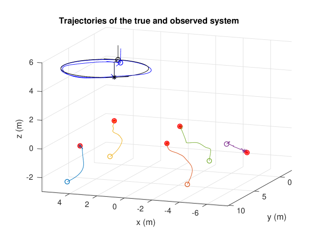
To verify the landmark observer design in Theorem 5.1 and the robot innovation term in Proposition 5.2, we conducted a simulation of a flying vehicle equipped with a monocular camera, observing 5 stationary landmarks as it moves in a circular trajectory with a constant body-fixed velocity $U=(\Omega_{U}^{\times},V_{U})$ , where $\Omega_{U}=(0,0,0.5)$ rad/s and $V_{U}=(1.5,0,0)$ m/s. For simplicity, it is assumed that the camera frame coincides with the body-fixed frame of the vehicle. The initial position of the vehicle was set to $(3,3,5)$ m with its rotational axes aligned with the inertial frame $\{0\}$ . The positions of the landmark are initialised to random positions $(p^{1}_{i},p^{2}_{i},0)$ on the ground plane with $p^{1}_{i},p^{2}_{i}\sim N(0,5^{2})$ m.

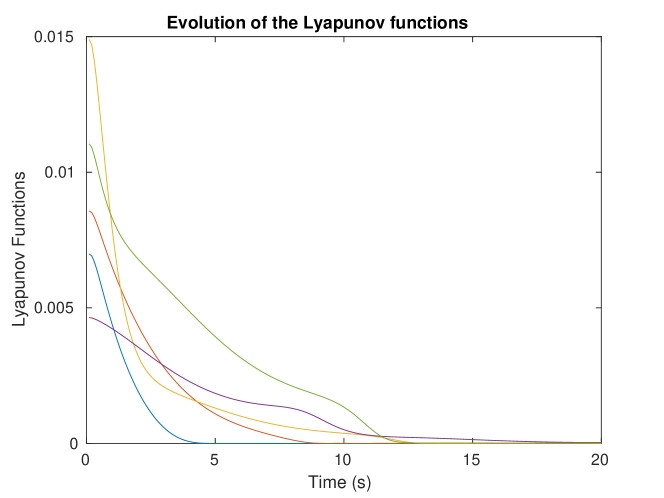
The origin position $P^{\circ}$ of the robot is set to the identity $I_{4}$ , and the origin landmark positions $p^{\circ}_{i}$ are set to $10y_{i}(0)$ , where $y_{i}(0)$ are the measured bearings to the true landmark positions at time 0. That is, the estimated points are initialised with correct bearings and an arbitrary depth of 10 m. The observer is defined on $\mathbf{VSLAM}_{5}(3)$ with kinematics given by (5.1), landmark innovation terms $(\Gamma_{i},\gamma_{i})$ given by (5.1), where $k_{i}=5$ and $\alpha_{i}=500$ , and robot innovation term $\Delta$ given as in Proposition 5.2 with $k_{i}=1$ . At the end of the simulation, the estimated system state is aligned with the true system state by matching the true and estimated robot poses. Figure 2 shows the trajectories of estimated landmark positions and robot position over time, as well as the true landmark positions and the true robot trajectory, and figure 3 shows the evolution of each of the landmarks’ associated storage functions, as defined in (21).

This simulation provides a simple demonstration of performance of the proposed observer and illustrates typical trajectories of the landmark estimates during a repeating motion such as the circle. The estimated landmark positions can be seen to converge to the true landmark positions in a natural manner. The choice to initialise landmarks as having a bearing matching the initial measurement is a natural one for practical implementation of the algorithm, although Theorem 5.1 provides that almost any initial conditions will converge. This almost semi-global convergence is a key property of the observer presented here that is not available in many of the state-of-art solutions.

7 Experimental Results

To demonstrate the observer described in Theorem 5.1 in a real-world scenario, we gathered video, GPS, and IMU data from a Disco Parrot fixed-wing UAV flying outdoors. Image features were identified using OpenCV’s goodFeaturesToTrack, and subsequently tracked using OpenCV’s calcOpticalFlowPyrLK. These image features were then corrected for camera intrinsics and converted to spherical bearing coordinates before being used as landmark inputs to the observer. Landmarks are added to the system state after being observed for two frames so that their depths can be initialised from optical flow. When a landmark is no longer visible, it is removed from the observer state.

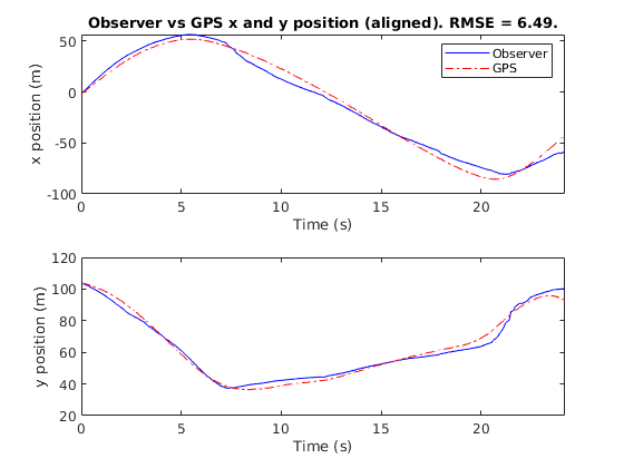
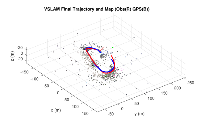
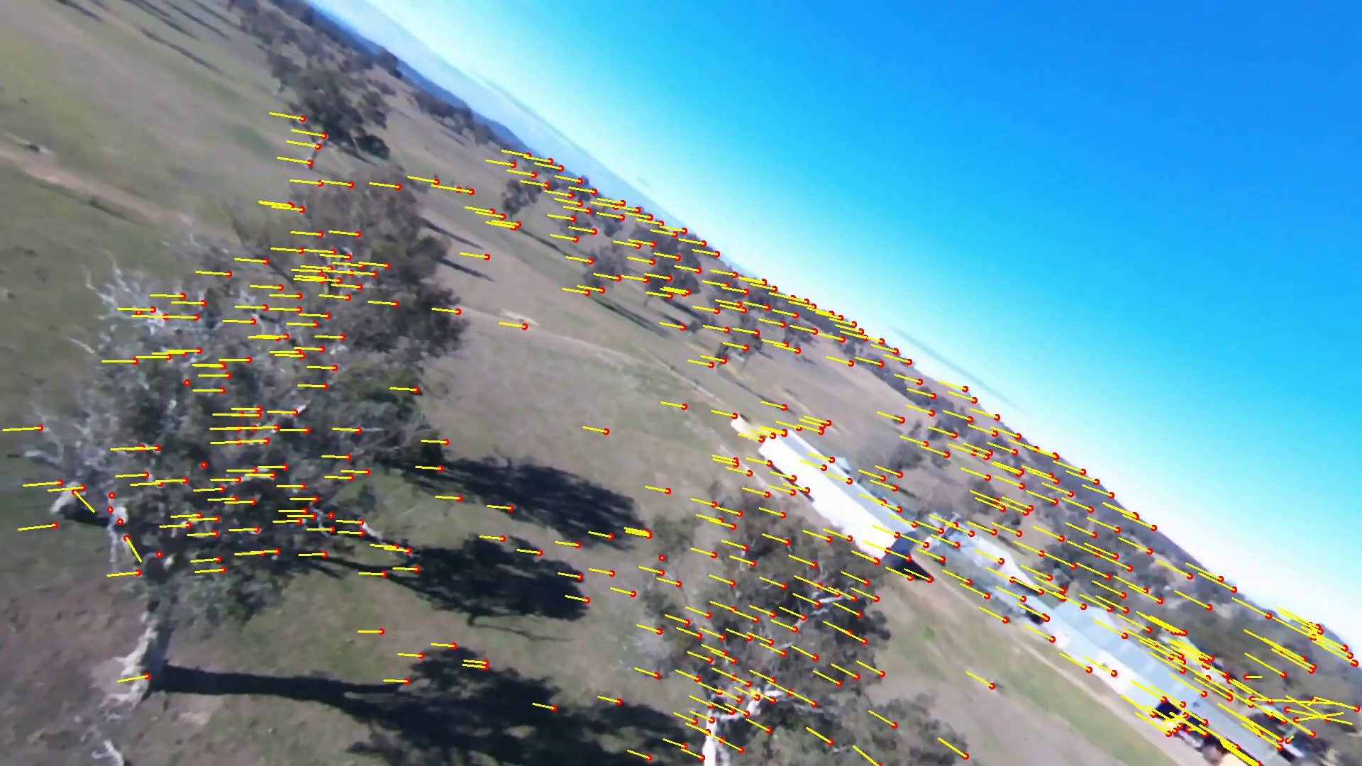
Initially, the input velocities $U=(\Omega_{U},V_{U})$ to the system were estimated by combining the GPS signal (to obtain scale information) with egomotion estimated using the IMU and optical flow from the video stream, as outlined in [18]. Once sufficiently many landmarks are initialised, the optical flow vectors of each of the landmarks were combined with the existing landmark estimates to compute the input velocity $U=(\Omega_{U},V_{U})$ . The observer was implemented using Euler integration with gain parameters set to $k_{i}=5.0$ and $\alpha_{i}=0.5$ for each $i$ . The video recorded had a frame rate of $30$ fps, leading to the Euler integration step being set to $\mathrm{d}t=0.033$ s. GPS data was recorded at $25$ Hz in order to compare with the observer’s estimated trajectory. The observer trajectory was aligned to the GPS trajectory using the Umeyama method [21]. Figure 4 shows the aligned trajectories according to the observer and according to the GPS in the $x$ and $y$ directions, where the $z$ direction refers to the plane’s altitude. Figure 5 shows the final positions of all landmark points in addition to the observer- and GPS-estimated trajectories. Figure 6 shows a frame taken from the video stream used in the experiment, with lines to represent the optical flow tracking overlaid. A video showcasing the feature tracking system is available online¹¹1https://www.youtube.com/watch?v=QzIxh2eM1_s.

8 Conclusion

This paper presents an observer design posed on a symmetry group for the VSLAM problem. The SLAM manifold introduced in [16] and the symmetry group discussed in [22] are reintroduced and exploited in the observer design. The observer is formulated on output errors, and provides a clear way to change the gains for bearing and depth of landmarks separately. The almost semi-global convergence of the proposed observer improves on the properties of state-of-the-art Extended Kalman Filter systems, which suffer from linearisation errors. While research into the development of non-linear observers for the SLAM problem is only recent, the observer for VSLAM presented in this paper demonstrates some of the key advantages the approach can offer.

Appendix A Almost Semi-Global Asymptotic Stabilising Controls and Innovations

The concept of semi-global asymptotic stabilisability was introduced in [20] to model the dependence of gain on the basin of attraction in feedback stabilisation of a dynamical system. In the context of an observer analysis, this definition can be transferred to stabilisability of the error dynamics by innovation. However, the classical concept introduced by Teel and Praly does not capture topological constraints associated with stability analysis on manifolds. For a large class of manifolds, including Lie-groups with $\mathbf{SO}(3)$ as a subgroup, these topological constraints prevent the existence of globally smooth asymptotically stable error dynamics [3]. On such spaces, smooth error dynamics will always admit an exception set $\chi$ of unstable or hyperbolic critical points that cannot be part of the basin of attraction of the desired equilibrium.

We consider a system-observer pair, where the observer has the internal model principle, coupled through an innovation function $\Delta(\hat{x},y)$ depending on the observer state and system output. We assume that there is a well defined error function $e:\mathbf{G}\times\mathcal{M}\to\mathcal{M}$ where $\mathbf{G}$ is the observer state space and $\mathcal{M}$ is the system state space. The error dynamics evolve on the manifold $\mathcal{M}$ depending on the system and observer state evolution as well as any exogenous inputs such as velocities.

Definition A.1.

An equilibrium $e_{\star}$ of the error dynamics of a system-observer pair, on a manifold $\mathcal{M}$ , is almost globally stable if its basin of attraction is the complement of an exception set $\chi\subset\mathcal{M}$ of measure zero.

An equilibrium $e_{\star}$ of the error dynamics of a observer-system pair, on a manifold $\mathcal{M}$ , is said to be almost semi-globally stabilizable if, for each compact set $K\subset\mathcal{M}$ in the complement of an exception set $\chi\subset\mathcal{M}$ of measure zero, there exist a choice of innovation $\Delta(\hat{x},y)$ such that $e_{\star}$ is an asymptotically stable equilibrium of the error dynamics with basin of attraction containing $K$ .

Acknowledgement

This research was supported by the Australian Research Council through the “Australian Centre of Excellence for Robotic Vision” CE140100016.

References

[1] G. Baldwin, R. Mahony, and J. Trumpf. A nonlinear observer for 6 DOF pose estimation from inertial and bearing measurements. In Proceedings of the IEEE International Conference on Robotics and Automation (ICRA), pages 2237–2242, 2009.
[2] Axel Barrau and Silvere Bonnabel. An EKF-SLAM algorithm with consistency properties, 2016. arXiv:1510.06263.
[3] S.P. Bhata and D.S. Bernstein. Atopological obstruction to continuous global stabilization of rotational motion and the unwinding phenomenon. Systems & Control Letters, 39:63–70, 2000.
[4] E. Bjorne, T. A. Johansen, and E. F. Brekke. Redesign and analysis of globally asymptotically stable bearing only SLAM. In 2017 20th International Conference on Information Fusion (Fusion), pages 1–8, July 2017.
[5] S. Bonnabel, P. Martin, and P. Rouchon. Symmetry-preserving observers. IEEE Transactions on Automatic Control, 53(11):2514–2526, 2008.
[6] F. Le Bras, T. Hamel, R. Mahony, and C. Samson. Observers for position and velocity bias estimation from single or multiple direction outputs. In T.I. Fossen, K.Y. Pettersen, and H. Nijmeijer, editors, Sensing and Control for Autonomous Vehicles, chapter 1. Lecture Notes in Control and Information Sciences 474, Springer, 2017.
[7] Martin Brossard, Silvere Bonnabel, and Axel Barrau. Unscented kalman filter on lie groups for visual inertial odometry. In 2018 IEEE/RSJ International Conference on Intelligent Robots and Systems (IROS), pages 649–655. IEEE, 2018.
[8] Cesar Cadena, Luca Carlone, Henry Carrillo, Yasir Latif, Davide Scaramuzza, José Neira, Ian Reid, and John J Leonard. Past, present, and future of simultaneous localization and mapping: Toward the robust-perception age. IEEE Transactions on robotics, 32(6):1309–1332, 2016.
[9] J. Delmerico and D. Scaramuzza. A benchmark comparison of monocular visual-inertial odometry algorithms for flying robots. In IEEE International Conference on Robotics and Automation (ICRA), 2018.
[10] Jorge Fuentes-Pacheco, José Ruiz-Ascencio, and Juan Manuel Rendón-Mancha. Visual simultaneous localization and mapping: a survey. Artificial Intelligence Review, 43(1):55–81, 2015.
[11] T. Hamel and C. Samson. Riccati observers for the nonstationary pnp problem. IEEE Transactions on Automatic Control, 63(3):726–741, March 2018.
[12] Minh-Duc Hua, Mohammad Zamani, Jochen Trumpf, Robert Mahony, and Tarek Hamel. Observer design on the special euclidean group SE(3). In Proceedings of the IEEE Conference on Decision and Control and European Control Conference, Orlando, FL, USA, December 2011.
[13] Pedro Lourenço, Bruno Guerreiro, Pedro Batista, Paulo Oliveira, and Carlos Silvestre. Simultaneous localization and mapping for aerial vehicles: a 3-d sensor-based gas filter. Autonomous Robots, 40(5):881–902, 2016.
[14] Pedro Lourenço, Pedro Batista, Paulo Oliveira, and Carlos Silvestre. A globally exponentially stable filter for bearing-only simultaneous localization and mapping with monocular vision. Robotics and Autonomous Systems, 100:61 – 77, 2018.
[15] R. Mahony, T. Hamel, and J. Pflimlin. Nonlinear complementary filters on the special orthogonal group. IEEE Transactions on Automatic Control, 53(5):1203–1218, June 2008.
[16] Robert Mahony and Tarek Hamel. A geometric nonlinear observer for simultaneous localisation and mapping. In Conference on Decision and Control, page 6 pages, Melbourne, December 2017.
[17] Robert Mahony, Jochen Trumpf, and Tarek Hamel. Observers for kinematic systems with symmetry. In Proceedings of 9th IFAC Symposium on Nonlinear Control Systems (NOLCOS), page 17 pages, 2013. Plenary paper.
[18] Felix Schill, Robert Mahony, and Peter Corke. Estimating ego-motion in panoramic image sequences with inertial measurements. In Robotics Research, pages 87–101. Springer, 2011.
[19] H. Strasdat, J.M.M. Montiel, and A.J. Davison. Visual SLAM: Why filter? Computer Vision and Image Understanding (CVIU), 30(2):65–77, 2012.
[20] A.R. Teel and L. Praly. Global stabilizability and observability imply semi-global stabilizability by output feedback. Systems and Control Letters, (22):313–325, 1994.
[21] S Umeyama. Least-squares estimation of transformation parameters between two point patterns. IEEE Transactions on Pattern Analysis and Machine Intelligence, 13(4):376–380, 1991.
[22] Pieter van Goor, Robert Mahony, Tarek Hamel, and Jochen Trumpf. A geometric observer design for visual localisation and mapping. In 2019 IEEE 58th Conference on Decision and Control (CDC), pages 2543–2549. IEEE, 2019.
[23] J.F. Vasconcelos, R. Cunha, C. Silvestre, and P. Oliveira. A nonlinear position and attitude observer on SE(3) using landmark measurements. Systems & Control Letters, 59(3-4):155–166, 2010.
[24] David Evan Zlotnik and James Richard Forbes. Gradient-based observer for simultaneous localization and mapping. IEEE Transactions on Automatic Control, 63(12):4338–4344, 2018.

Constructive Observer Design for Visual Simultaneous Localisation and Mapping

Abstract

1 Introduction

2 Preliminaries

2.1 Notation

3 Problem Formulation

3.1 VSLAM State Space

3.2 VSLAM Kinematics

3.3 System Output

4 Symmetry of the VSLAM Problem

4.1 Symmetry of the Total Space 𝒯n∘​(3)\mathcal{T}^{\circ}_{n}(3)

Lemma 4.1.

Proof.

4.2 Symmetry of the Output Space

Proposition 4.2.

Proof.

Lemma 4.3.

Proof.

4.3 Lift of the VSLAM Kinematics

Lemma 4.4.

Proof.

5 Observer Design

5.1 Lifted System Kinematics

5.2 Landmark Observer

Theorem 5.1.

Proof.

5.3 Total Space Representative

Proposition 5.2.

Proof.

6 Simulation Results

7 Experimental Results

8 Conclusion

Appendix A Almost Semi-Global Asymptotic Stabilising Controls and Innovations

Definition A.1.

Acknowledgement

References

4.1 Symmetry of the Total Space $\mathcal{T}^{\circ}_{n}(3)$