Construction of unstable concentrated solutions of the Euler and gSQG equations

Martin Donati¹¹1Univ. Grenoble Alpes, Institut Fourier, F-38000 Grenoble, France. Contact : [email protected].

Abstract

In this paper we construct solutions to the Euler and gSQG equations that are concentrated near unstable stationary configurations of point-vortices. Those solutions are themselves unstable, in the sense that their localization radius grows from order $\varepsilon$ to order $\varepsilon^{\beta}$ (with $\beta<1$ ) in a time of order $|\ln\varepsilon|$ . This proves in particular that the logarithmic lower-bound obtained in previous papers (in particular [P. Buttà and C. Marchioro, Long time evolution of concentrated Euler flows with planar symmetry, SIAM J. Math. Anal., 50(1):735–760, 2018]) about vorticity localization in Euler and gSQG equations is optimal. In addition we construct unstable solutions of the Euler equations in bounded domains concentrated around a single unstable stationary point. To achieve this we construct a domain whose Robin’s function has a saddle point.

^†^†2020 Mathematics Subject Classification : 76B47, 34A34^†^†Keywords : Point-vortex dynamics, Euler equations, SQG equations, Vorticity localization, Long time confinement, Hyperbolic critical point

1 Introduction

We are interested in this paper in different active scalar equations from fluid dynamics: the two-dimensional incompressible Euler equations, used to describe an inviscid and incompressible fluid; and the Surface Quasi Geostrophic (SQG) equations, used as a model of geophysical flows. We also consider the generalized Surface Quasi-Geostrophic equations (gSQG) that interpolates between the Euler equations and the SQG equations. Let $\omega:\mathbb{R}^{2}\to\mathbb{R}$ be the active scalar, which we will refer to as the vorticity as in the Euler equations, and $u:\mathbb{R}^{2}\to\mathbb{R}^{2}$ be the velocity of the fluid. Then the Euler equations, the SQG equations and the gSQG equations in the plane can all be written in the form

\begin{cases}\partial_{t}\omega(x,t)+u\cdot\nabla\omega(x,t)=0,&\forall(x,t)\in\mathbb{R}^{2}\times(0,+\infty)\\ u(x,t)=\nabla^{\perp}\Delta^{-s}(\omega)(x,t),&\forall(x,t)\in\mathbb{R}^{2}\times[0,+\infty)\\ u(x,t)\to 0,&\text{as }|x|\to+\infty,\hskip 5.69046pt\forall t\in[0,+\infty)\\ \omega(x,0)=\omega_{0}(x),&\forall x\in\mathbb{R}^{2},\end{cases}

with $s\in[\frac{1}{2},1]$ . The Euler equations correspond to the case $s=1$ , the SQG equations to the case $s=\frac{1}{2}$ , and the gSQG equations are the family $s\in(\frac{1}{2},1)$ . For details on the geophysical model see for instance [24, 28]. Let us recall that the fundamental solution of $\Delta^{s}$ in the plane is given for $x\neq y$ by

G_{s}(x,y)=\begin{cases}\frac{1}{2\pi}\ln|x-y|&\text{ if $s=1$},\\ \frac{\Gamma(1-s)}{2^{2s}\,\pi\,\Gamma(s)}\frac{1}{|x-y|^{2-2s}}&\text{ if $\frac{1}{2}\leq s<1$},\end{cases}

where $\Gamma$ is the standard Gamma function. Therefore for every $s\in(\frac{1}{2},1]$ there exists a constant $C_{s}$ such that

\nabla_{x}G_{s}(x,y)=C_{s}\frac{x-y}{|x-y|^{4-2s}}.

This motivates us to define $\alpha:=3-2s$ , so that $|\nabla_{x}G_{\alpha}(x,y)|\leq C_{\alpha}|x-y|^{-\alpha}$ , for $\alpha\in[1,2)$ and the appropriate choice of $C_{\alpha}$ . In conclusion, the equations that we consider are the family of equations

\begin{cases}\partial_{t}\omega(x,t)+u(x,t)\cdot\nabla\omega(x,t)=0,\vspace{2mm}\\ \displaystyle u(x,t)=\int_{\mathbb{R}^{2}}C_{\alpha}\frac{(x-y)^{\perp}}{|x-y|^{\alpha+1}}\omega(y,t)\mathrm{d}y,\\ \omega(x,0)=\omega_{0}(x).\end{cases}

(1)

We recall that the Euler case corresponds to $s=\alpha=1$ . We observe that we necessarily have that $\nabla\cdot u=0$ when it makes sense. When $\alpha\geq 2$ , the kernel cease to be $L^{1}_{\mathrm{loc}}$ so the Biot-Savart law in (1) does not make sense anymore. In that case the Biot-Savart law should be expressed differently, see for instance [19]. In this paper we only consider $\alpha\in[1,2)$ .

For the Euler equations, we have global existence and uniqueness of both strong solutions, and weak solutions in $L^{1}\cap L^{\infty}$ from the Yudovitch theorem [29]. When $\alpha\in(1,2)$ , from [13], we know the existence, but not uniqueness, of weak solutions in $L^{1}\cap L^{\infty}$ of equations (1). The existence of strong solutions is only known locally in time, and the blow-up of the SQG equations is an important open problem.

In this paper we construct families of particular initial data $\omega_{0}$ such that any (since it may not be unique) solution of (1) satisfies various constraints. These functions $\omega_{0}$ always lie in $L^{1}\cap L^{\infty}$ , but can also be taken $C^{\infty}$ . Hence when $\alpha=1$ , the solution remains $C^{\infty}$ for all time, but in general, we can only consider global in time $L^{1}\cap L^{\infty}$ solutions of (1).

We now focus on the particular situation where the active scalar is concentrated into small blobs as follows. We denote by $D(z,r)$ the disk of radius $r$ centered in $z$ . We consider solutions $\omega$ satisfying

\omega=\sum_{i=1}^{N}\omega_{i}\hskip 5.69046pt\text{ and }\hskip 5.69046pt\mathrm{supp}\hskip 2.84526pt\omega_{i}\subset D(z_{i}(t),r(t)),

with $r(t)$ being small in some sense. A classical model to describe concentrated solutions of equations (1) is the point-vortex model. The principle is to approximate the blob $\omega_{i}$ by the Dirac mass $a_{i}\delta_{z_{i}(t)}$ , where the intensity

a_{i}=\int_{\mathbb{R}^{2}}\omega_{i}(x,t)\mathrm{d}x,

is constant in time²²2See [13] Corollary 2.7 for the case of weak solutions. For strong solutions this is a direct consequence of the fact that $\nabla\cdot u=0$ , see for instance [21].. The dynamics of those Dirac masses, that we call point-vortices, is then given by the system

\forall i\in\llbracket 1,N\rrbracket,\quad\frac{\mathrm{d}}{\mathrm{d}t}z_{i}(t)=C_{\alpha}\sum_{\begin{subarray}{c}1\leq j\leq N\\ j\neq i\end{subarray}}a_{j}\frac{(z_{i}(t)-z_{j}(t))^{\perp}}{|z_{i}(t)-z_{j}(t)|^{\alpha+1}}.

(

\alpha

-PVS)

This system of equations is often called $\alpha$ -point-vortex system, or $\alpha$ -model. We recall that this model is mathematically justified, see for instance [22, 27, 26, 2, 6] for the Euler case and [13, 25, 15, 5] for the gSQG case. In particular, on a finite time interval $[0,T]$ , if no collisions of point-vortices occurs, then if

\omega_{0,\varepsilon}\underset{\varepsilon\to 0}{\longrightarrow}\sum_{i=1}^{N}a_{i}\delta_{z_{i}(0)}

weakly in the sense of measures, then

\omega_{\varepsilon}(t)\underset{\varepsilon\to 0}{\longrightarrow}\sum_{i=1}^{N}a_{i}\delta_{z_{i}(t)},

where the $t\mapsto z_{i}(t)$ are the solutions of the point-vortex dynamics. This means that point-vortices are a singular limit of solutions of the associated PDE. Fore a more detailed introduction of the point-vortex system, we refer the reader to [21].

2 Vorticity confinement and main results

We now introduce the long time vorticity confinement problem, recall some important theorems on the subject and state our main results.

2.1 Long time confinement problem

We define the long time confinement problem as the following – see [2]. Let $N\in\mathbb{N}^{*}$ and $\varepsilon>0$ . For each $i\in\{1,\ldots,N\}$ let $z_{i}^{*}\in\mathbb{R}^{2}$ chosen pairwise distinct and $a_{i}\in\mathbb{R}^{*}=\mathbb{R}\setminus\{0\}$ . Assume that $\omega_{0}$ is such that

\begin{cases}\displaystyle\omega_{0}=\sum_{i=1}^{N}\omega_{0,i}\hskip 5.69046pt\text{ and }\hskip 5.69046pt\mathrm{supp}\hskip 2.84526pt\omega_{0,i}\subset D(z_{i}^{*},\varepsilon),\vspace{1mm}\\ \displaystyle\omega_{0,i}\text{ has a sign}\hskip 5.69046pt\text{ and }\hskip 5.69046pt\int_{\mathbb{R}^{2}}\omega_{0,i}(x)\mathrm{d}x=a_{i},\vspace{1mm}\\ \displaystyle|\omega_{0}|\leq C\varepsilon^{-\nu},\quad\text{ for some }\nu\geq 2,\vspace{1mm}\\ \displaystyle|z_{i}^{*}(t)-z_{j}^{*}(t)|>0,\quad\forall t\in[0,+\infty),\end{cases}

(2)

were we denote by $z_{i}^{*}(t)$ the associated solution of the point-vortex dynamics with initial data $z_{i}^{*}(0)=z_{i}^{*}$ and intensities $a_{i}$ . The last hypothesis ensures that the point-vortex dynamics has a global in time solution: no collision occurs. This is not a very restrictive hypothesis since it is known that the point-vortex system has a global solution for almost any initial data, in the sense of the Lebesgue measure. This was proved for the Euler point-vortex dynamics (namely equations ( $\alpha$ -PVS) for $\alpha=1$ ) in the torus [10], in bounded domains [7] and in the plane³³3With an additional hypothesis on the intensities: $\sum_{i\in P}a_{i}\neq 0$ , for any $P\subset\{1,\ldots,N\}$ , with $P\neq\emptyset$ . This hypothesis was then weakened in [14] to $P\neq\{1,\ldots,N\}$ . [20]. For the general $\alpha$ -model ( $\alpha$ -PVS) it was proved in the plane⁴⁴4With the same additional hypothesis. [4, 14].

Let $\beta<1$ . We introduce the exit time:

\tau_{\varepsilon,\beta}=\sup\left\{t\geq 0\text{ such that }\forall s\in[0,t],\hskip 5.69046pt\mathrm{supp}\hskip 2.84526pt\omega(\cdot,s)\subset\bigcup_{i=1}^{N}D(z_{i}^{*}(s),\varepsilon^{\beta})\right\}.

The long time confinement problem consists in obtaining a lower-bound on $\tau_{\varepsilon,\beta}$ in order to describe how long the approximation of a concentrated solution of equations (1) by the point-vortex model ( $\alpha$ -PVS) remains valid. Results have been obtained in [2, 8, 5]. In the following, we recall some of them and state our main results, starting with the case $\alpha=1$ .

2.2 Result for Euler equations in the plane

A first general result was obtained in [2].

Theorem 2.1 (Marchioro-Buttà, [2]).

Let $\beta<1/2$ . Then there exists $\xi_{0}>0$ such that for every $\varepsilon>0$ small enough, for any $\omega_{0}$ satisfying (2) for some $\nu\geq 2$ , the solution $\omega$ of the Euler equations satisfies

\tau_{\varepsilon,\beta}>\xi_{0}|\ln\varepsilon|.

In special cases, this can be improved. For instance, with the same hypotheses than those of Theorem 2.1, but assuming furthermore that $N=1$ , one can easily obtain that $\tau_{\varepsilon,\beta}\geq\varepsilon^{-\xi_{0}}$ , for some $\xi_{0}>0$ . An extension of this result is the following.

Theorem 2.2 (Marchioro-Buttà, [2]).

Let $\beta<1/2$ . Then there exists $\xi_{0}>0$ and a configuration of point-vortices, namely a choice of $a_{i}$ and $z_{i}^{*}$ , such that for any $\varepsilon>0$ small enough and for any $\omega_{0}$ satisfying (2), the solution $\omega$ of the Euler equations satisfies

\tau_{\varepsilon,\beta}>\varepsilon^{-\xi_{0}}.

The configuration is a self-similar expanding configuration of three point-vortices. The key point is that as point-vortices move far from each other, their mutual influence decreases with time.

In this paper, we want to prove that the logarithmic bound obtained in Theorems 2.1 is optimal, namely that there are solutions of (1) satisfying (2) such that $\tau_{\varepsilon,\beta}\leq\xi_{1}|\ln\varepsilon|$ . We prove the following result.

Theorem 2.3.

There exists $\beta_{0}<1/2$ , $\nu\geq 2$ and a configuration $\big{(}(z_{i}^{*})_{i},(a_{i})_{i}\big{)}$ of point-vortices with $N=3$ such that for every $\beta\in(\beta_{0},1)$ , for any $\xi_{1}>\frac{4\pi}{3}(1-\beta)$ and for every $\varepsilon>0$ small enough there exists $\omega_{0}$ satisfying (2) such that the solution $\omega$ of the Euler equations in the plane satisfies

\tau_{\varepsilon,\beta}\leq\xi_{1}|\ln\varepsilon|.

This confirms that the logarithmic bound obtained in Theorems 2.1 is optimal.

2.3 Result for the gSQG equations in the plane

A result similar to Theorem 2.1 has been obtained for the gSQG equations.

Theorem 2.4 (Cavallaro-Garra-Marchioro, [5]).

Let $\alpha\in(1,2)$ and $\beta$ such that $0<\beta<\frac{4-2\alpha}{5-\alpha}<\frac{1}{2}$ . Then there exists $\xi_{0}>0$ such that for every $\varepsilon>0$ small enough, for any $\omega_{0}$ satisfying (2) with $\nu=2$ and for any $\omega$ a weak solution of (1) we have that

\tau_{\varepsilon,\beta}>\xi_{0}|\ln\varepsilon|.

Remark 2.5.

Please note that in the hypotheses of Theorem 2.4 is assumed that $\nu=2$ , which is not in the hypotheses of Theorem 2.1. Actually, we claim that in their proof of Theorem 2.4, the authors of [5] only need to assume the existence of $\nu\geq 2$ , and not $\nu=2$ . This is due to Lemma 2.4 of [5].

We then prove the following.

Theorem 2.6.

Let $\alpha\in[1,2)$ . Then there exists $\nu\geq 2$ , an initial configuration $\big{(}(z_{i}^{*})_{i},(a_{i})_{i}\big{)}$ of point-vortices with $N=3$ , and $\beta_{0}<\frac{4-2\alpha}{5-\alpha}$ such that for every $\beta\in(\beta_{0},1)$ , for every $\xi_{1}>\frac{1-\beta}{C_{\alpha}(2-2^{-\alpha})\sqrt{\alpha}}$ and for every $\varepsilon>0$ small enough there exists $\omega_{0}$ satisfying (2) such that any solution $\omega$ of (1) satisfies

\tau_{\varepsilon,\beta}\leq\xi_{1}|\ln\varepsilon|.

This confirms that the logarithmic bound obtained in Theorems 2.4 is optimal.

Remark 2.7.

Both in Theorems 2.3 and 2.6, the lower-bound for $\xi_{1}$ is not optimal. Moreover, $\omega_{0}$ is localized initially in a disk of size $\varepsilon$ but the size of its support is of order $\varepsilon^{\nu/2}$ . In Appendix C, we give details how concentrated the initial data needs to be depending on the construction, and give examples constructions involving more point-vortices, which improve the bounds for $\xi_{1}$ and $\nu$ .

2.4 Results for the Euler equations in bounded domains

In a second part of this paper, we turn to a new situation. We focus on the Euler equations, namely the case $\alpha=1$ , but in a bounded domain $\Omega$ . Let us recall the Euler equations in a bounded and simply connected domain $\Omega\subset\mathbb{R}^{2}$ :

\begin{cases}\partial_{t}\omega+u\cdot\nabla\omega=0,\vspace{2mm}\\ \displaystyle u=\nabla^{\perp}\Delta^{-1}\omega,\\ u\cdot n=0,&\text{ on }\partial\Omega,\\ \omega(x,0)=\omega_{0}(x),&\text{ on }\Omega.\end{cases}

(Eu)

When being far from the boundary, one can express the effect of the boundary as a Lipschitz exterior field. This trick makes it very easy to extend Theorem 2.1 to the case of bounded domains – as it is suggested in [2].

In that same article, the authors proved that when the initial vorticity is concentrated near the center of a disk, namely that $\Omega=D(0,1)$ , $N=1$ and $z_{1}=0$ , then we obtain the same power-law lower-bound $\tau_{\varepsilon,\beta}\geq\varepsilon^{-\xi_{0}}$ than with expanding self-similar configurations. This result has been generalized to other bounded domains in [8]. This is due to a strong stability property induced by the shape of the boundary. Here we are interested in the opposite situation: we construct a domain whose boundary creates an instability. We then obtain a third and final result, different from Theorems 2.3 and 2.6 because it only involves a single blob.

Theorem 2.8.

There exists a smooth bounded domain $\Omega$ and $\beta_{0}<1/2$ such that for every $\beta\in(\beta_{0},1)$ , for every $\xi_{1}>(1-\beta)\frac{2\pi}{\sqrt{3}}$ and every $\varepsilon>0$ small enough, there exists $\omega_{0}$ satisfying (2) with $N=1$ and $\nu=4$ such that the solution $\omega$ of (Eu) satisfies

\tau_{\varepsilon,\beta}\leq\xi_{1}|\ln\varepsilon|.

We prove Theorems 2.3, 2.6 and 2.8 using the same plan: we construct a solution of the point-vortex dynamics that move away from its initial position exponentially fast, then construct a solution concentrated around it in the sense of hypothesis (2).

The paper is organized as follows. In Section 3 we give several definitions and expose in details the plan of the proofs and the main tools. In Section 4 we do the explicit construction to prove Theorems 2.3 and 2.6. Finally in Section 5 we prove Theorem 2.8.

3 Outline of the proofs

In this section we expose the main tools required for the proofs of our results. Before going any further, let us introduce some notation.

In the rest of the paper,

•

$|z|$ , for $z\in\mathbb{R}^{2}$ designates the usual $2$ -norm, or modulus,
•

$z^{\perp}=(-z_{2},z_{1})$ ,
•

$|Z|_{\infty}$ for $Z=(z_{1},\ldots,z_{N})\in(\mathbb{R}^{2})^{N}$ designates $\max_{1\leq i\leq N}|z_{i}|$ ,
•

$C$ is a name reserved for constants whose value is not relevant, and may change from line to line,
•

$D(z,r)$ is the disk (in $\mathbb{R}^{2}$ ) or radius $r$ centered in $z$ .

Please notice that our construction – in particular $\omega_{0}$ – depends on $\varepsilon$ , though we do not write the dependence of each quantity in $\varepsilon$ for the sake of legibility.

3.1 Plan

The proofs of Theorems 2.3, 2.6 and 2.8 rely on two main steps. We first look for an unstable stationary configuration of point-vortices. Then we control the behaviour of a well prepared solution initially concentrated around this configuration.

Let us give some details on each step.

Step 1: constructing an unstable vortex configuration.

We consider the dynamical system $\frac{\mathrm{d}}{\mathrm{d}t}Z(t)=f(Z(t))$ . Then we say that $Z^{*}$ is a stationary point of the dynamics if $f(Z^{*})=0$ , and that it is unstable if $\mathrm{D}f(Z^{*})$ has an eigenvalue with positive real part.

At this step, we first aim to choose $N$ , $\Omega$ (when necessary), the family of $a_{i}$ and $z_{i}^{*}$ . The trick is following: we choose intensities $a_{i}\in\mathbb{R}^{*}$ and a point $Z^{*}=(z_{1}^{*},\ldots,z_{N}^{*})\in(\mathbb{R}^{2})^{N}$ which is a stationary and unstable initial datum of the point-vortex dynamics ( $\alpha$ -PVS). Let us notice that choosing a stationary configuration $Z^{*}$ ensures that the hypothesis $|z_{i}^{*}(t)-z_{j}^{*}(t)|>0$ for all $t\geq 0$ is always satisfied. The consequence of the instability is that for every $\varepsilon>0$ , there exists an initial configuration of point-vortices $Z_{0}$ such that

|Z^{*}-Z_{0}|_{\infty}=\frac{\varepsilon}{2},

and the solution $t\mapsto Z(t)$ such that $Z(0)=Z_{0}$ move away exponentially fast from $Z^{*}$ , therefore implying that for any $\beta<1$ ,

\tau_{Z}:=\sup\left\{t\geq 0\text{ such that }\forall s\in[0,t]\;,\;|Z(s)-Z^{*}|_{\infty}\leq 2\varepsilon^{\beta}\right\}\leq\xi_{0}|\ln\varepsilon|.

This problem is much simpler than the original one since we are investigating the behaviour of solutions of a system of ordinary differential equations, the point-vortex dynamics, instead of a solution of a partial derivative equation. More precisely, we have the following proposition, obtained as a corollary of Theorem 6.1, Chapter 9 of [17], and proved in Section 3.3.

Proposition 3.1.

Let $f:(\mathbb{R}^{2})^{N}\to(\mathbb{R}^{2})^{N}$ . We consider the differential equation

\frac{\mathrm{d}}{\mathrm{d}t}Z(t)=f(Z(t)).

(3)

Assume that there exists $Z^{*}\in(\mathbb{R}^{2})^{N}$ such that $f(Z^{*})=0$ . Assume furthermore that $\mathrm{D}f(Z^{*})$ has an eigenvalue with positive real part $\lambda_{0}>0$ .

Then for any $\lambda<\lambda_{0}$ , for every $\varepsilon>0$ small enough and for any $\beta\in(0,1)$ there exists and a choice of $Z_{0}$ such that $|Z_{0}-Z^{*}|_{\infty}=\varepsilon/2$ ,

\tau_{Z}\leq\frac{1-\beta}{\lambda}|\ln\varepsilon|.

In conclusion, proving that $\tau_{Z}\leq\xi_{1}|\ln\varepsilon|$ simply relies on finding an eigenvalue with positive real part of the Jacobian matrix of the dynamic’s functional.

Step 2: constructing the approximation

The idea is then to prove that a solution $\omega$ with well prepared initial data $\omega_{0}$ satisfying (2) satisfies that for every $t\leq\tau_{\varepsilon,\beta}$ ,

|B(t)-Z(t)|_{\infty}=o(\varepsilon^{\beta}),

where

B_{i}(t)=\frac{1}{a_{i}}\int_{\mathbb{R}^{2}}x\omega_{i}(x,t)\mathrm{d}x,

and $B(t)=(B_{1}(t),\ldots,B_{N}(t))$ . The conclusion then comes from the fact that by construction (Step 1), there exists $t_{1}\leq\frac{1-\beta}{\lambda}$ such that $|Z(t_{1})-Z^{*}|_{\infty}=2\varepsilon^{\beta}$ and thus for $\varepsilon$ small enough, $\tau_{\varepsilon,\beta}\leq t_{1}\leq\xi_{1}|\ln\varepsilon|$ .

In order to obtain this control on $|B(t)-Z(t)|_{\infty}$ , we need to estimate the moment of inertia

I_{i}(t)=\frac{1}{a_{i}}\int_{\mathbb{R}^{2}}|x-B_{i}(t)|^{2}\omega_{i}(x,t)\mathrm{d}x

of each blob. The constant $\nu$ in (2) intervenes when estimating $I(0)$ . The critical part in this step is the competition between the growth of $I_{i}$ , which loosen the control on $|B(t)-Z(t)|_{\infty}$ , with the growth of $|Z(t)-Z^{*}|_{\infty}$ . When we do not have constraints on $\nu$ , then one can always choose $\nu$ large enough so that $I_{i}$ remains small long enough. However the difficulty arises when wanting to construct $\omega_{0}$ with $\nu=4$ . This requires to be able to estimate precisely the growth of each $I_{i}$ , of $|Z(t)-Z^{*}|_{\infty}$ and of $|B(t)-Z(t)|_{\infty}$ .

All of this is captured in Theorem 3.2 presented in Section 3.2.

3.2 Confinement around an unstable configuration

Once the unstable configuration of point-vortices is obtained in Step 1, most of the work needed in the second step does not depend on that configuration nor on the specific framework. Therefore, we establish a general theorem that we will be able to apply for any suitable configuration of vortices, also including when appropriate the presence of a boundary.

To understand better the dynamics of each blob, we describe the influence of the other blobs or of the boundary by an an exterior field. We assume that each blob is a solution of a problem

\begin{cases}\partial_{t}\omega_{i}(x,t)+\big{(}u_{i}(x,t)+F_{i}(x,t)\big{)}\cdot\nabla\omega_{i}(x,t)=0,\vspace{2mm}\\ \displaystyle u_{i}(x,t)=\int_{\mathbb{R}^{2}}C_{\alpha}\frac{(x-y)^{\perp}}{|x-y|^{\alpha+1}}\omega_{i}(y,t)\mathrm{d}y,\vspace{1mm}\\ \omega_{i}(x,0)=\omega_{i,0}(x),\\ \end{cases}

(4)

where $F_{i}$ is an exterior field that satisfies $\nabla\cdot F_{i}=0$ . Let $Z^{*}\in(\mathbb{R}^{2})^{N}$ and $f\in C^{1}\Big{(}(\mathbb{R}^{2})^{N}\,,\,(\mathbb{R}^{2})^{N}\Big{)}$ such that $f(Z^{*})=0$ . We write $f=(f_{1},\ldots,f_{N})$ . For any $Z_{0}$ , let $t\mapsto Z(t)$ be the solution of the problem

\begin{cases}\displaystyle\frac{\mathrm{d}}{\mathrm{d}t}Z(t)=f(Z(t))\vspace{1mm}\\ Z(0)=Z_{0}.\end{cases}

(5)

In this particular setting, for any $\beta\in(0,1)$ , we have

\tau_{\varepsilon,\beta}=\sup\left\{t\geq 0\text{ such that }\forall s\in[0,t],\hskip 5.69046pt\mathrm{supp}\hskip 2.84526pt\omega(\cdot,s)\subset\bigcup_{i=1}^{N}D(z_{i}^{*},\varepsilon^{\beta})\right\}.

Assuming that $|Z_{0}-Z^{*}|_{\infty}=\varepsilon/2$ , we recall that

\tau_{Z}:=\sup\left\{t\geq 0\text{ such that }\forall s\in[0,t]\;,|Z(s)-Z^{*}|_{\infty}<2\varepsilon^{\beta}\right\}.

We then have the following theorem.

Theorem 3.2.

Let $N\in\mathbb{N}^{*}$ , $a_{i}\in\mathbb{R}^{*}$ for every $i\in\{1,\ldots,N\}$ , $Z^{*}\in(\mathbb{R}^{2})^{N}$ . Let $f\in C^{1}\big{(}(\mathbb{R}^{2})^{N},(\mathbb{R}^{2})^{N}\big{)}$ and $F_{i}$ such that $\nabla\cdot F_{i}=0$ . We assume the following.

$(i)$

$f(Z^{*})=0$ and $\mathrm{D}f(Z^{*})$ has an eigenvalue with positive real part $\lambda_{0}$ ,
$(ii)$

There exists $C$ such that for all $i\in\{1,\ldots,N\}$ , $\forall t\leq\tau_{\varepsilon,\beta}$ ,

$\left|F_{i}(B_{i}(t),t)-f_{i}(B(t))\right|\leq C\sum_{j=1}^{N}\sqrt{I_{j}},$
$(iii)$

There exists constants $\kappa_{0}$ , $\kappa_{1}$ and $\kappa_{2}$ such that $\forall i\in\{1,\ldots,N\}$ , $\forall\,x,x^{\prime}\in D(z_{i}^{*},\varepsilon^{\beta})$ , $\forall\,t\leq\tau_{\varepsilon,\beta}$ ,

$|F_{i}(x,t)-F_{i}(x^{\prime},t)|\leq\kappa_{0}|x-x^{\prime}|,$ (6)

and

$\Big{|}(x-x^{\prime})\cdot\big{(}F_{i}(x,t)-F_{i}(x^{\prime},t)\big{)}\Big{|}\leq\kappa_{1}|x-x^{\prime}|^{2},$ (7)

and $\forall\,X,X^{\prime}\in(\mathbb{R}^{2})^{N}$ such that $|X-Z^{*}|_{\infty}\leq 2\varepsilon^{\beta}$ and $|X^{\prime}-Z^{*}|_{\infty}\leq 2\varepsilon^{\beta}$ ,

$|f(X)-f(X^{\prime})|_{\infty}\leq\kappa_{2}|X-X^{\prime}|_{\infty}.$ (8)

Then there exists $\nu\geq 2$ and $\beta_{0}<\frac{4-2\alpha}{5-\alpha}$ such that for all $\beta\in(\beta_{0},1)$ , for every $\xi>\frac{1-\beta}{\lambda_{0}}$ and for every $\varepsilon>0$ small enough, there exists $\omega_{0}$ satisfying (2) such that any $\omega=\sum_{i=1}^{N}\omega_{i}$ solution of the problem (4) for every $i$ satisfies

\tau_{\varepsilon,\beta}\leq\xi|\ln\varepsilon|.

Proof.

First, we use Hypothesis $(i)$ to apply Proposition 3.1 and get that for every $\varepsilon$ small enough, there exists $Z_{0}$ such that $|Z_{0}-Z^{*}|_{\infty}=\varepsilon/2$ and for every $\beta\in(0,1)$ , the solution $Z$ of the problem (5) satisfies

\tau_{Z}\leq\frac{1-\beta}{\lambda}|\ln\varepsilon|.

(9)

Now let $\omega_{0}$ satisfying (2) for some $\nu\geq 2$ and such that

B(0)=Z_{0},

(10)

and

\forall i\in\{1,\ldots,N\},\quad I_{i}(0)\leq\varepsilon^{\nu}.

(11)

This is always possible as stated in Remark B.1 given in Appendix B. Let $\omega=\sum_{i=1}^{N}\omega_{i}$ such that each $\omega_{i}$ is a solution of the problem (4).

We observe that if $\tau_{\varepsilon,\beta}\leq\tau_{Z}$ , then we have the desired result. So for the sake of contradiction, we can assume that $\tau_{\varepsilon,\beta}>\tau_{Z}$ .

Recalling that $\omega_{i}$ solves (4), we have that

\frac{\mathrm{d}}{\mathrm{d}t}B_{i}=\frac{1}{a_{i}}\int F_{i}(x,t)\omega_{i}(x,t)\mathrm{d}x

and

\frac{\mathrm{d}}{\mathrm{d}t}I_{i}=\frac{2}{a_{i}}\int(x-B_{i}(t))\cdot(F_{i}(x,t)-F_{i}(B_{i}(t),t))\omega_{i}(x,t)\mathrm{d}x.

Indeed, if $\omega_{i}$ is smooth (when $\alpha=1$ or before a possible regularity blow-up if $\alpha>1$ ), these are classical computations. In general, $\omega_{i}\in L^{1}\cap L^{\infty}$ and these relations hold in the weak sense, see for instance [13, Corollary 2.8] or [5].

Now using Hypothesis $(iii)$ , and observing from (2) that $\frac{\omega_{i}}{a_{i}}\geq 0$ , we get that

\left|\frac{\mathrm{d}}{\mathrm{d}t}I_{i}\right|\leq 2\kappa_{1}\int|x-B_{i}(t)|^{2}\frac{\omega_{i}(x,t)}{a_{i}}\mathrm{d}x=2\kappa_{1}I_{i}(t).

Therefore, we get that

I_{i}(t)\leq I_{i}(0)e^{2\kappa_{1}t}.

(12)

We now want to estimate $|B(t)-Z(t)|_{\infty}$ . For every $i\in\{1,\ldots,N\}$ we have that

	$\displaystyle\left\|\frac{\mathrm{d}}{\mathrm{d}t}B_{i}(t)-f_{i}(B(t))\right\|$	$\displaystyle=\left\|\frac{1}{a_{i}}\int\big{(}F_{i}(x,t)-f_{i}(B(t))\big{)}\omega_{i}(x,t)\mathrm{d}x\right\|$
		$\displaystyle=\left\|\frac{1}{a_{i}}\int\big{(}F_{i}(x,t)-F_{i}(B_{i}(t),t)+F_{i}(B_{i}(t),t)-f_{i}(B(t))\big{)}\omega_{i}(x,t)\mathrm{d}x\right\|$
		$\displaystyle\leq\kappa_{0}\int\|x-B_{i}(t)\|\frac{\omega_{i}(x,t)}{a_{i}}\mathrm{d}x+C\sum_{j=1}^{N}\sqrt{I_{j}(t)},$

where we used hypotheses $(ii)$ and $(iii)$ . By the Cauchy Schwartz inequality we have that

\int|x-B(t)|\frac{\omega_{i}(x,t)}{a_{i}}\mathrm{d}x=\left(\int|x-B(t)|^{2}\frac{\omega_{i}(x,t)}{a_{i}}\mathrm{d}x\right)^{1/2}\left(\int\frac{\omega_{i}(x,t)}{a_{i}}\mathrm{d}x\right)^{1/2}\leq\sqrt{I_{i}(t)},

and therefore, since the result is now uniform in $i$ ,

\left|\frac{\mathrm{d}}{\mathrm{d}t}B(t)-f(B(t))\right|_{\infty}\leq C\sum_{j=1}^{N}\sqrt{I_{j}(t)}.

The value of $C$ is irrelevant and changes from line to line. The value of $\kappa_{0}$ is also irrelevant in the end and is absorbed in $C$ .

We recall that by relation (10), $B(0)=Z_{0}=Z(0)$ and that $Z$ is a solution of the problem (5) with $f$ being a Lipschitz map by Hypothesis $(iii)$ . We now use a variant of the Gronwall’s inequality – Lemma B.2 given in appendix – to obtain that

\big{|}B(t)-Z(t)\big{|}_{\infty}\leq Ce^{\kappa_{2}t}\int_{0}^{t}\sum_{j=1}^{N}\sqrt{I_{j}(s)}\mathrm{d}s.

Using relation (12), we have that

\sum_{j=1}^{N}\int_{0}^{t}\sqrt{I_{j}(s)}\mathrm{d}s\leq\sum_{j=1}^{N}\int_{0}^{t}\sqrt{I_{j}(0)}e^{\kappa_{1}s}\mathrm{d}s\leq\sum_{j=1}^{N}\frac{\sqrt{I_{j}(0)}}{\kappa_{1}}e^{\kappa_{1}t}.

Recalling that by relation (11), $I_{j}(0)\leq\varepsilon^{\nu}$ , we obtain that

\big{|}B(t)-Z(t)\big{|}_{\infty}\leq C\varepsilon^{\nu/2-(\kappa_{1}+\kappa_{2})t|\ln\varepsilon|}.

We are interested in proving that $\forall t\leq\tau_{Z}$ ,

\big{|}B(t)-Z(t)\big{|}_{\infty}=o(\varepsilon^{\beta}),

(13)

as $\varepsilon\to 0$ . For $\varepsilon<1$ and for all $t\leq\tau_{Z}$ , by relation (9), for any $\lambda<\lambda_{0}$ ,

-t|\ln\varepsilon|\geq\frac{1-\beta}{\lambda}.

Therefore, one sufficient condition to obtain (13) is

\nu>2\frac{\kappa_{1}+\kappa_{2}}{\lambda_{0}}(1-\beta)+2\beta,

(14)

since in that case, one can choose $\lambda$ close enough to $\lambda_{0}$ such that

\nu/2-\frac{\kappa_{1}+\kappa_{2}}{\lambda}(1-\beta)>\beta.

We observe that necessarily, $\kappa_{2}\geq\lambda_{0}$ so $\frac{\kappa_{1}+\kappa_{2}}{\lambda_{0}}>1$ and therefore the map $\phi:\beta\mapsto 2\frac{\kappa_{1}+\kappa_{2}}{\lambda_{0}}(1-\beta)+2\beta$ is decreasing on $[0,1]$ . Let

\nu>\phi\left(\frac{4-2\alpha}{5-\alpha}\right)=\frac{2}{5-\alpha}\left((1+\alpha)\frac{\kappa_{1}+\kappa_{2}}{\lambda_{0}}+4-2\alpha\right).

(15)

Since $\phi$ is also continuous, then there exists $\beta_{0}<\frac{4-2\alpha}{5-\alpha}$ such that $\forall\beta\in(\beta_{0},1)$ ,

\nu>\phi(\beta).

In particular, for every $\beta\in(\beta_{0},1)$ , relation (14) holds true and thus relation (13) too.

We conclude by observing that for $\varepsilon$ small enough,

|B(\tau_{Z})-Z^{*}|_{\infty}\geq|Z(\tau_{Z})-Z^{*}|_{\infty}-|B(\tau_{Z})-Z(\tau_{Z})|_{\infty}\geq 2\varepsilon^{\beta}-o(\varepsilon^{\beta})\geq\varepsilon^{\beta}.

Since $\forall\,t<\tau_{\varepsilon,\beta}$ , we have that $|B(t)-Z^{*}|_{\infty}<\varepsilon^{\beta}$ by definition of $\tau_{\varepsilon,\beta}$ , the previous relation is in contradiction with $\tau_{\varepsilon,\beta}>\tau_{Z}$ . Therefore,

\tau_{\varepsilon,\beta}\leq\tau_{Z}\leq\frac{1-\beta}{\lambda}|\ln\varepsilon|,

for any $\lambda<\lambda_{0}$ . In particular, for every $\beta\in(\beta_{0},1)$ , for every $\xi_{1}>\frac{1-\beta}{\lambda_{0}}$ , we proved that for $\varepsilon$ small enough,

\tau_{\varepsilon,\beta}\leq\xi_{1}|\ln\varepsilon|.

∎

Let us mention that Hypothesis $(i)$ is a consequence of the choice of $Z^{*}$ and the $a_{i}$ made at Step 1, and that Hypothesis $(ii)$ is a consequence of the nature of the relation between the exterior fields $F_{i}$ and the map $f$ . Of course, the result could not be true if the $F_{i}$ and $f$ were not related to each other.

The existence of $\kappa_{0}$ , $\kappa_{1}$ and $\kappa_{2}$ in the Hypothesis $(iii)$ is a direct consequence of the fact that every $F_{i}$ and $f$ are Lipschitz maps, which will always be the case in our framework. Even though relation (7) is a consequence of (6), only $\kappa_{1}$ and $\kappa_{2}$ intervene in the condition (15) on $\nu$ . This is important when one wants to compute precisely the bounds on $\nu$ , as we do in Section 5, and for several other examples in Appendix C.

Finally, we notice that we actually proved that any solution $\omega$ starting from any initial data $\omega_{0}$ satisfying (2) and relations (10) and (11) satisfies $\tau_{\varepsilon,\beta}\leq\xi_{1}|\ln\varepsilon|$ . Therefore, there is a large family of initial data, in terms for instance of the shape of the blob, that solves our problem.

3.3 Proof of Proposition 3.1.

Let us recall Theorem 6.1, Chapter 9 of [17].

Theorem 3.3.

Let $f:(\mathbb{R}^{2})^{N}\to(\mathbb{R}^{2})^{N}$ . We consider the differential equation

\frac{\mathrm{d}}{\mathrm{d}t}Z(t)=f(Z(t)).

Assume that there exists $Z^{*}\in(\mathbb{R}^{2})^{N}$ is such that $f(Z^{*})=0$ . Assume furthermore that $\mathrm{D}f(Z^{*})$ has an eigenvalue with positive real part $\lambda_{0}>0$ . Then there exists a solution of (3) such that $Z(t)$ exists some fixed neighbourhood of $Z^{*}$ , that

Z(t)\underset{t\to-\infty}{\longrightarrow}Z^{*},

and that

\frac{1}{t}\ln|Z(t)-Z^{*}|_{\infty}\underset{t\to-\infty}{\longrightarrow}\lambda_{0}.

We now prove Proposition 3.1. Let $\beta\in(0,1)$ and let $\widetilde{Z}$ a solution of (3) given by Theorem 3.3. Since $\widetilde{Z}\underset{t\to-\infty}{\longrightarrow}Z^{*}$ and since $\widetilde{Z}$ exits some fixed neighbourhood of $Z^{*}$ , for $\varepsilon$ small enough, there exists $t_{0}$ and $t_{1}$ such that

\begin{cases}-\infty<t_{0}<t_{1}\\ t_{1}\to-\infty&\text{ as }\varepsilon\to 0\\ |\widetilde{Z}(t_{1})-Z^{*}|_{\infty}=2\varepsilon^{\beta}\\ |\widetilde{Z}(t_{0})-Z^{*}|_{\infty}=\varepsilon/2.\end{cases}

Let $Z(t)=\widetilde{Z}(t+t_{0})$ , we have that $|Z(0)-Z^{*}|_{\infty}=\varepsilon/2$ and that $\tau_{Z}\leq t_{1}-t_{0}$ since $Z(t_{1}-t_{0})=2\varepsilon^{\beta}$ . Moreover, since

\ln|Z(t)-Z^{*}|_{\infty}=\lambda_{0}t+o_{t\to-\infty}(t),

then for any $\eta\in(0,1)$ , for $-t$ big enough we have that

1-\eta<\frac{\ln|Z(t)-Z^{*}|_{\infty}}{\lambda_{0}t}<1+\eta

Therefore, for $\varepsilon$ small enough, applying in $t_{0}$ and $t_{1}$ (we recall that $t_{1}\to-\infty$ as $\varepsilon\to 0$ ) we have that

t_{1}<\frac{\ln|Z(t_{1})-Z^{*}|_{\infty}}{\lambda_{0}(1+\eta)}=\frac{\beta\ln\varepsilon+\ln 2}{\lambda_{0}(1+\eta)}=\frac{-\beta|\ln\varepsilon|+\ln 2}{\lambda_{0}(1+\eta)}

and

-t_{0}<-\frac{\ln|Z(t_{0})-Z^{*}|_{\infty}}{\lambda_{0}(1-\eta)}=\frac{|\ln\varepsilon|+\ln 2}{\lambda_{0}(1-\eta)}

and thus

t_{1}-t_{0}<|\ln\varepsilon|\left(\frac{1}{\lambda_{0}(1-\eta)}-\frac{\beta}{\lambda_{0}(1+\eta)}+\frac{\ln 2}{\lambda_{0}|\ln\varepsilon|}\left(\frac{1}{1+\eta}+\frac{1}{1-\eta}\right)\right).

Therefore, by letting $\eta\to 0$ , for any $\lambda<\lambda_{0}$ , for $\varepsilon$ small enough,

t_{1}-t_{0}\leq\frac{1-\beta}{\lambda}|\ln\varepsilon|.

By definition, $\tau_{Z}\leq t_{1}-t_{0}\leq\frac{1-\beta}{\lambda}|\ln\varepsilon|$ . This concludes the proof.

4 Unstable configurations of multiple vortices in the plane

In this section we show that we can choose a configuration $Z^{*}$ and intensities $a_{i}$ such that we can apply Theorem 3.2 to estimate the exit time $\tau_{\varepsilon,\beta}$ of a solution of the equations (1). Please notice that Theorem 2.3 is a direct consequence of Theorem 2.6 by taking $\alpha=1$ . Therefore, we work with some general $\alpha\in[1,2)$ .

We start by introducing a family of point-vortex configurations $Z^{*}$ for any $N\geq 3$ . We then construct the exterior fields $F_{i}$ such that the blobs $\omega_{i}$ is a solution of the problem (4), and start proving each of the conditions to apply Theorem 3.2. We then prove Theorem 2.3, and Proposition C.1 by computing explicitly the properties of our construction with $N=3$ . In Appendix C, we use the construction with $N=7$ and $N=9$ .

4.1 Vortex crystals

Let us introduce a family of stationary solutions of the $\alpha$ -point-vortex model ( $\alpha$ -PVS) that are part of the so called vortex crystals family. For a more general study of vortex crystals and their stability, we refer the reader to [1, 23, 3]. Fore the sake of legibility, we identify $\mathbb{C}=\mathbb{R}^{2}$ for the position of point-vortices. We use the notation $x=\big{(}(x)_{p},(x)_{q}\big{)}=(x)_{p}+i(x)_{q}$ .

Let $N\geq 3$ , and

K_{\alpha}(x,y)=C_{\alpha}\frac{(x-y)^{\perp}}{|x-y|^{\alpha+1}},

so that the point-vortex equation ( $\alpha$ -PVS) becomes

\forall i\in\llbracket 1,N\rrbracket,\quad\frac{\mathrm{d}}{\mathrm{d}t}z_{i}(t)=\sum_{\begin{subarray}{c}1\leq j\leq N\\ j\neq i\end{subarray}}a_{j}K_{\alpha}\big{(}z_{i}(t),z_{j}(t)\big{)}.

In particular, by setting for all $Z=(z_{1},\ldots,z_{N})$ :

f(Z)=\left(\sum_{j\neq i}a_{j}K_{\alpha}(z_{i},z_{j})\right)_{1\leq i\leq N},

then we have that

\frac{\mathrm{d}}{\mathrm{d}t}Z(t)=f(Z(t)).

We consider $N$ point-vortices in the following configuration. The first $N-1$ points form a regular $(N-1)$ -polygon, and the $N$ -th vortex is placed at the center. For instance, by letting $\zeta=e^{i\frac{2\pi}{N-1}}$ , where here $i$ denotes the complex unit, we set

	$\displaystyle\forall j\in\{1,\ldots,N-1\},\hskip 5.69046ptz_{j}^{*}=\zeta^{j},$	$\displaystyle\quad a_{j}=1$
	$\displaystyle z_{N}^{*}=0,$	$\displaystyle\quad a_{N}\in\mathbb{R}.$

Then, (see for instance [1]) the solution of ( $\alpha$ -PVS) with initial configuration $Z^{*}=(z_{1}^{*},\ldots,z_{N}^{*})$ satisfies $z_{j}(t)=e^{i\mu t}z_{j}^{*}$ for some angular velocity $\nu$ that does not depend on $j$ . The motion of the whole configuration is a rigid rotation around 0, which makes it a so called vortex crystal.

This stands for any choice of $a_{N}\in\mathbb{R}$ . Now we make a particular choice. For every $N\geq 3$ , there exists $a_{N}\neq 0$ in the previous configuration such that the solution is stationary ( $\mu=0$ ). Indeed, let us compute the velocity of any point vortex (except the one at the center that is always stationary), for instance $z_{N-1}=\zeta^{N-1}=1$ .

	$\displaystyle\frac{\mathrm{d}}{\mathrm{d}t}z_{N-1}(0)$	$\displaystyle=\sum_{j=1}^{N-2}K_{\alpha}(1,\zeta^{j})+a_{N}K_{\alpha}(1,0)$
		$\displaystyle=C_{\alpha}\left(\sum_{j=1}^{N-2}\frac{(1-\zeta^{j})}{\|1-\zeta^{j}\|^{\alpha+1}}+a_{N}\right)^{\perp}.$

Since $\overline{\zeta^{j}}=\zeta^{N-1-j}$ , the quantity $\sum_{j=1}^{N-2}\frac{(1-\zeta^{j})}{|1-\zeta^{j}|^{\alpha+1}}$ is a non vanishing real number and thus letting

a_{N}=-\sum_{j=1}^{N-2}\frac{(1-\zeta^{j})}{|1-\zeta^{j}|^{\alpha+1}}

enforces that $\frac{\mathrm{d}}{\mathrm{d}t}z_{N-1}(0)=0$ . By symmetry, $\frac{\mathrm{d}}{\mathrm{d}t}z_{j}(0)=0$ for every $j\in{1,\ldots,N-1}$ . As for $z_{N}$ , it is always stationary, again by a symmetry argument, or by a simple computation.

In conclusion, for any $N\geq 3$ , we constructed a $N$ -vortex configuration that is stationary. In order to study the stability of the equilibrium $Z^{*}$ , we compute $\mathrm{D}f(Z^{*})$ . To this end, let us compute

	$\displaystyle\frac{1}{C_{\alpha}}$	$\displaystyle\big{(}K_{\alpha}(z_{i}+x,z_{j}+y)-K_{\alpha}(z_{i},z_{j})\big{)}$
		$\displaystyle=\frac{\big{(}(z_{i}+x)-(z_{j}+y)\big{)}^{\perp}}{\big{\|}(z_{i}+x)-(z_{j}+y)\big{\|}^{\alpha+1}}-\frac{(z_{i}-z_{j})^{\perp}}{\|z_{i}-z_{j}\|^{\alpha+1}}$
		$\displaystyle=\frac{(z_{i}-z_{j})^{\perp}}{\big{\|}(z_{i}+x)-(z_{j}+y)\big{\|}^{\alpha+1}}-\frac{(z_{i}-z_{j})^{\perp}}{\|z_{i}-z_{j}\|^{\alpha+1}}+\frac{(x-y)^{\perp}}{\big{\|}(z_{i}+x)-(z_{j}+y)\big{\|}^{\alpha+1}}$
		$\displaystyle=\frac{(z_{i}-z_{j})^{\perp}}{\|z_{i}-z_{j}\|^{\alpha+1}}\left(1-(\alpha+1)(x-y)\cdot\frac{z_{i}-z_{j}}{\|z_{i}-z_{j}\|^{2}}+o\big{(}\|x\|+\|y\|\big{)}-1\right)+\frac{(x-y)^{\perp}}{\|z_{i}-z_{j}\|^{\alpha+1}}+o\big{(}\|x\|+\|y\|\big{)},$

and finally, we obtain that

\frac{1}{C_{\alpha}}\big{(}K_{\alpha}(z_{i}+x,z_{j}+y)-K_{\alpha}(z_{i},z_{j})\big{)}\\ =-\frac{(z_{i}-z_{j})^{\perp}}{|z_{i}-z_{j}|^{\alpha+3}}(\alpha+1)(x-y)\cdot(z_{i}-z_{j})+\frac{(x-y)^{\perp}}{|z_{i}-z_{j}|^{\alpha+1}}+o\big{(}|x|+|y|\big{)}.

(16)

Since each coordinate $z_{i}$ of $f$ is of dimension two, we need some clarification on the notations. We now think of $f$ as the map

\widetilde{f}:\begin{cases}\mathbb{R}^{2N}\to\mathbb{R}^{2N}\\ \big{(}p_{1},q_{1},\ldots,p_{N},q_{N}\big{)}\mapsto\big{(}\widetilde{f}_{p_{1}},\widetilde{f}_{q_{1}},\ldots,\widetilde{f}_{p_{N}},\widetilde{f}_{q_{N}}\big{)}=f\big{(}p_{1}+iq_{1},\ldots,p_{N}+iq_{N}\big{)}.\end{cases}

Relation (16) yields for $i\neq j$ that

\begin{cases}\displaystyle\frac{1}{a_{j}C_{\alpha}}\partial_{p_{j}}\widetilde{f}_{p_{i}}=-\frac{(z_{i}-z_{j})_{q}}{|z_{i}-z_{j}|^{\alpha+3}}(\alpha+1)(z_{i}-z_{j})_{p}\vspace{1mm}\\ \displaystyle\frac{1}{a_{j}C_{\alpha}}\partial_{p_{j}}\widetilde{f}_{q_{i}}=\frac{(z_{i}-z_{j})_{p}}{|z_{i}-z_{j}|^{\alpha+3}}(\alpha+1)(z_{i}-z_{j})_{p}-\frac{1}{|z_{i}-z_{j}|^{\alpha+1}}\vspace{1mm}\\ \displaystyle\frac{1}{a_{j}C_{\alpha}}\partial_{q_{j}}\widetilde{f}_{p_{i}}=-\frac{(z_{i}-z_{j})_{q}}{|z_{i}-z_{j}|^{\alpha+3}}(\alpha+1)(z_{i}-z_{j})_{q}+\frac{1}{|z_{i}-z_{j}|^{\alpha+1}}\vspace{1mm}\\ \displaystyle\frac{1}{a_{j}C_{\alpha}}\partial_{q_{j}}\widetilde{f}_{q_{i}}=\frac{(z_{i}-z_{j})_{p}}{|z_{i}-z_{j}|^{\alpha+3}}(\alpha+1)(z_{i}-z_{j})_{q},\end{cases}

and for $i=j$ ,

\begin{cases}\displaystyle\partial_{p_{i}}\widetilde{f}_{p_{i}}=-\sum_{j\neq i}\partial_{p_{j}}\widetilde{f}_{p_{i}}\vspace{1mm}\\ \displaystyle\partial_{p_{i}}\widetilde{f}_{q_{i}}=-\sum_{j\neq i}\partial_{p_{j}}\widetilde{f}_{q_{i}}\vspace{1mm}\\ \displaystyle\partial_{q_{i}}\widetilde{f}_{p_{i}}=-\sum_{j\neq i}\partial_{q_{j}}\widetilde{f}_{p_{i}}\vspace{1mm}\\ \displaystyle\partial_{q_{i}}\widetilde{f}_{q_{i}}=-\sum_{j\neq i}\partial_{q_{j}}\widetilde{f}_{q_{i}}.\end{cases}

In order to keep the notations as light as possible, we will write $\mathrm{D}f$ in place of $\mathrm{D}\widetilde{f}$ .

4.2 Defining the exterior fields

We recall that in order to apply Theorem 3.2, we need to show that every blob $\omega_{i}$ is a solution of a problem (4) with some exterior field $F_{i}$ .

Let $\omega_{0}$ satisfying the general hypotheses (2) for $N\geq 3$ and $Z^{*}$ the stationary vortex crystal presented in Section 4.1. Let $\omega$ be a solution of (1). We observe that each blob $\omega_{i}$ is solution of (1) by letting

F(x,t)=F_{i}(x,t)=\int\sum_{j\neq i}K_{\alpha}(x,y)\omega_{j}(y,t)\mathrm{d}y.

Since $\nabla_{x}\cdot K_{\alpha}(x,y)=0$ , then $\nabla\cdot F=0$ . Moreover, we have the following lemma, that proves that Hypothesis $(ii)$ of Theorem 3.2 is satisfied.

Lemma 4.1.

Let $i\in\{1,\ldots,N\}$ . We have for all $t\leq\tau_{\varepsilon,\beta}$ that

\big{|}F_{i}(B_{i}(t),t)-f_{i}(B(t))\big{|}\leq C\sum_{j=1}^{N}\sqrt{I_{j}},

where $C$ depends only on $\alpha$ , the $a_{i}$ and $Z^{*}$ .

Proof.

	$\displaystyle\left\|F_{i}(B_{i}(t),t)-f_{i}(B(t))\right\|$	$\displaystyle=\left\|\sum_{j\neq i}\int K_{\alpha}(B_{i}(t),y)\omega_{j}(y,t)\mathrm{d}y-\sum_{j\neq i}a_{j}K_{\alpha}(B_{i}(t),B_{j}(t))\right\|$
		$\displaystyle=\left\|\sum_{j\neq i}\int\big{(}K_{\alpha}(B_{i}(t),y)-K_{\alpha}(B_{i}(t),B_{j}(t))\big{)}\omega_{j}(y,t)\mathrm{d}y\right\|$
		$\displaystyle\leq\sum_{j\neq i}\int\big{\|}K_{\alpha}(B_{i}(t),y)-K_{\alpha}(B_{i}(t),B_{j}(t))\big{\|}\frac{\|a_{j}\|\omega_{j}(y,t)}{a_{j}}\mathrm{d}y$
		$\displaystyle\leq C\sum_{j\neq i}\|a_{j}\|\int\big{\|}y-B_{j}(t)\big{\|}\frac{\omega_{j}(y,t)}{a_{j}}\mathrm{d}y$
		$\displaystyle\leq C\sum_{j\neq i}\sqrt{I_{j}(t)},$

where we used that $K_{\alpha}$ and its derivatives are smooth on $\mathbb{R}^{2}\times\mathbb{R}^{2}\setminus\{x=y\}$ , and go to 0 when $|x-y|\to+\infty$ , so in particular $K_{\alpha}$ is a Lipschitz map on $\bigcup_{i\neq j}D(z_{i}^{*},\varepsilon^{\beta})\times D(z_{j}^{*},\varepsilon^{\beta})$ . ∎

The existence of $\kappa_{0}$ , $\kappa_{1}$ and $\kappa_{2}$ is trivial since $F$ and $f$ are Lipschitz maps while the blobs and point-vortices remain far from each other, which is always the case when $t\leq\tau_{\varepsilon,\beta}$ and $t\leq\tau_{Z}$ , so Hypothesis $(iii)$ is always satisfied.

Therefore, in order to apply Theorem 3.2, we come down to prove that there is indeed an eigenvalue of $\mathrm{D}f(Z^{*})$ with positive real part. Then the only remaining difficult task is to estimate the constants $\kappa_{1}$ , $\kappa_{2}$ and $\lambda_{0}$ to obtain an information on the lowest possible choice of $\nu$ .

4.3 Proof of Theorems 2.3 and 2.6

We now prove Proposition C.1, which in turns proves Theorem 2.3. We construct explicitly the vortex crystal as described in Section 4.1 with $N=3$ , namely the configuration:

\begin{cases}z_{1}^{*}=(-1,0),&a_{1}=1\\ z_{2}^{*}=(1,0),&a_{2}=1\\ z_{3}^{*}=(0,0),&a_{3}=-\frac{1}{2^{\alpha}}.\end{cases}

We now compute $\mathrm{D}f(Z^{*})$ using the method previously described at the end of Section 4.1 to obtain the $6\times 6$ matrix:

\mathrm{D}f(Z^{*})=C_{\alpha}\left(\begin{array}[]{cccccc}0&2^{-(\alpha+1)}&0&2^{-(\alpha+1)}&0&-2^{-\alpha}\\ 2^{-(\alpha+1)}\alpha&0&2^{-(\alpha+1)}\alpha&0&-2^{-\alpha}\alpha&0\\ 0&2^{-(\alpha+1)}&0&2^{-(\alpha+1)}&0&-2^{-\alpha}\\ 2^{-(\alpha+1)}\alpha&0&2^{-(\alpha+1)}\alpha&0&-2^{-\alpha}\alpha&0\\ 0&1&0&1&0&-2\\ \alpha&0&\alpha&0&-2\alpha&0\\ \end{array}\right)

The eigenvalues of this matrix are 0, with multiplicity 4, and $\pm C_{\alpha}(2-2^{-\alpha})\sqrt{\alpha}$ . So by letting $\lambda_{0}=C_{\alpha}(2-2^{-\alpha})\sqrt{\alpha}$ we have here a positive eigenvalue, associated with the eigenvector

v_{\lambda_{0}}=\left(-1,\sqrt{\alpha},-1,\sqrt{\alpha},-2^{\alpha+1},\sqrt{\alpha}2^{\alpha+1}\right).

This conclude Step 1.

We now apply Theorem (3.2) and obtain the existence for any $\alpha\in[1,2)$ of $\nu\geq 2$ and $\beta_{0}<\frac{4-2\alpha}{5-\alpha}$ such that for every $\beta\in(\beta_{0},1)$ , every

\xi_{1}>\frac{1-\beta}{\lambda_{0}}=\frac{1-\beta}{C_{\alpha}(2-2^{-\alpha})\sqrt{\alpha}}

and every $\varepsilon>0$ small enough, there exists $\omega_{0}$ satisfying (2) such that any solution $\omega$ of (1) satisfies

\tau_{\varepsilon,\beta}\leq\xi_{1}|\ln\varepsilon|.

We proved Theorem 2.6, and by taking $\alpha=1$ we proved Theorem 2.3 as well.

5 Unstable point-vortex in a bounded domain

In this section we construct a bounded domain $\Omega$ and an initial data $\omega_{0}$ satisfying (2) with $N=1$ , such that the solution of (Eu) satisfies that

\tau_{\varepsilon,\beta}\leq\xi_{1}|\ln\varepsilon|,

for $\varepsilon$ small enough and for some $\xi_{1}$ . Since $N=1$ , we denote by $z^{*}=z_{1}^{*}=Z^{*}$ and $a=a_{1}$ .

We start by recalling some facts about the point-vortex dynamics in bounded domain, then we construct the domain. Finally, we prove Theorem 2.8 using again Theorem 3.2.

5.1 Euler equations and point-vortices in bounded domains

For the rest of the paper, we consider the Euler equations (Eu), which differs from before in the sense that now $\alpha=s=1$ , and $\omega:\Omega\to\mathbb{R}$ , where $\Omega$ is a bounded simply connected subset of $\mathbb{R}^{2}$ . We now recall that the problem

\begin{cases}\Delta\Psi=\omega&\quad\text{on }\Omega\\ \Psi=0&\quad\text{on }\partial\Omega\end{cases}

has a unique solution

\Psi(x)=\int_{\Omega}G_{\Omega}(x,y)\omega(y)\mathrm{d}y,

where $G_{\Omega}:\Omega\times\Omega\setminus\{x=y\}\to\mathbb{R}$ is the Green’s function of $-\Delta$ with Dirichlet condition in the domain $\Omega$ . Therefore, we have the Biot-Savart law:

u(x,t)=\int_{\Omega}\nabla_{x}^{\perp}G_{\Omega}(x,y)\omega(y,t)\mathrm{d}y.

An important property of the Green’s function $G_{\Omega}$ is that it decomposes as

G_{\Omega}=G_{\mathbb{R}^{2}}+\gamma_{\Omega},

where

G_{\mathbb{R}^{2}}(x,y)=\frac{1}{2\pi}\ln|x-y|,

and $\gamma_{\Omega}:\Omega\times\Omega\to\mathbb{R}_{+}$ harmonic in both variables. We denote by $\widetilde{\gamma}_{\Omega}:x\mapsto\gamma_{\Omega}(x,x)$ the Robin’s function of the domain $\Omega$ . This map plays a crucial role in the study of the point-vortex dynamics in bounded domain. Indeed, the point-vortices in move according to the system

\forall i\in\llbracket 1,N\rrbracket,\quad\frac{\mathrm{d}}{\mathrm{d}t}z_{i}(t)=\sum_{\begin{subarray}{c}1\leq j\leq N\\ j\neq i\end{subarray}}a_{j}\frac{\big{(}z_{i}(t)-z_{j}(t)\big{)}^{\perp}}{\big{|}z_{i}(t)-z_{j}(t)\big{|}^{2}}+\sum_{j=1}^{N}a_{j}\nabla^{\perp}_{x}\gamma_{\Omega}\big{(}z_{i}(t),z_{j}(t)\big{)},

which in the case $N=1$ reduces to

\frac{\mathrm{d}}{\mathrm{d}t}z(t)=\frac{a}{2}\nabla^{\perp}\widetilde{\gamma}_{\Omega}(z(t)).

Our plan to prove Theorem 2.8 is the same as the proof of Theorem 2.3. The aim is to apply Proposition3.1 and Theorem 3.2. We then straight away notice that when $\omega_{0}$ satisfy (2) with $N=1$ , and thus $\omega$ (which we can extend by 0 to $\mathbb{R}^{2}$ ) is constituted of a unique blob that solves (4) by setting

F(x,t)=\int\nabla_{x}^{\perp}\gamma_{\Omega}(x,y)\omega(y,t)\mathrm{d}y,

and $z$ is a solution of (5) by setting

f(z)=\frac{a}{2}\nabla^{\perp}\widetilde{\gamma}_{\Omega}(z(t)).

Therefore, we are looking for $z^{*}$ an unstable critical point of the Robin’s function $\widetilde{\gamma}_{\Omega}$ , namely such that $\nabla\widetilde{\gamma}_{\Omega}(z^{*})=0$ and $\mathrm{D}\nabla^{\perp}\widetilde{\gamma}_{\Omega}(z^{*})$ has a positive eigenvalue. However the Robin’s function is not known explicitly in general, and the existence of such a point depends on the domain $\Omega$ . Fortunately, we recall that for any simply connected domain $\Omega$ and for any $z^{*}\in\Omega$ , there exists a biholomorphic map $T:\Omega\to D:=D(0,1)$ such that $T(z_{0})=0$ . Such a map also satisfy that

\forall x\neq y\in\Omega,\quad G_{\Omega}(x,y)=G_{D}\big{(}T(x),T(y)\big{)},

and thus

\widetilde{\gamma}_{\Omega}(x)=\widetilde{\gamma}_{D}(x)+\frac{1}{2\pi}\ln|T^{\prime}(x)|.

5.2 Known results on critical points of the Robin’s function

In this section we refer to [8] and recall the following results. For more details on the Robin’s function we refer the reader to [16, 12].

Proposition 5.1 ([8], Proposition 2.4).

If $T:\Omega\to D$ is a biholomorphic map such that $T(z^{*})=0$ , then

\nabla\widetilde{\gamma}_{\Omega}(z^{*})=0\Longleftrightarrow T^{\prime\prime}(z^{*})=0.

In particular, if the domain $\Omega$ has two axes of symmetry, then the intersection $z^{*}$ necessarily satisfy $\nabla\widetilde{\gamma}_{\Omega}(z^{*})=0$ and thus $T^{\prime\prime}(z^{*})=0$ . For the time being, we assume the existence of such $z^{*}$ and state some of its properties.

Lemma 5.2 ([8], Lemma 4.1).

Let $T:\Omega\to D(0,1)$ and $z^{*}\in\Omega$ such that $T(z^{*})=0$ and $T^{\prime\prime}(z^{*})=0$ , then for every $\varepsilon>0$ small enough,

\forall x,y,z\in D(z^{*},\varepsilon^{\beta}),\quad\left|\nabla_{x}^{\perp}\gamma_{\Omega}(x,y)-\nabla_{x}^{\perp}\gamma_{\Omega}(z,y)\right|=|x-z|\left(\frac{|T^{\prime\prime\prime}(z^{*})|}{6\pi|T^{\prime}(z^{*})|}+\mathcal{O}\left(\varepsilon^{\beta}\right)\right).

The direct corollary of this lemma is that $F$ satisfies (7) with

\kappa_{1}=|a|\frac{|T^{\prime\prime\prime}(z^{*})|}{6\pi|T^{\prime}(z^{*})|}+o(1).

Proposition 5.3 ([8], Sections 3.2 and 3.3).

Let $\Omega\subset\mathbb{R}^{2}$ be a bounded simply connected domain. Then for any biholomorphism $T:\Omega\to D$ mapping $z^{*}$ to $0$ such that $T^{\prime\prime}(z^{*})=0$ , the hessian matrix $\mathrm{D}^{2}\widetilde{\gamma}_{\Omega}(z^{*})$ has non degenerate eigenvalues of opposite signs if and only if $|T^{\prime\prime\prime}(z^{*})|>2|T^{\prime}(z^{*})|^{3}$ . In that case, these eigenvalues are

\lambda_{\pm}=\frac{2|T^{\prime}(z^{*})|^{2}\pm|T^{\prime\prime\prime}(z^{*})|/|T^{\prime}(z^{*})|}{2\pi},

and the eigenvalues of $\mathrm{D}\nabla^{\perp}\widetilde{\gamma}_{\Omega}(z^{*})$ are $\pm\sqrt{-\lambda_{+}\lambda_{-}}$ , so that

\lambda_{0}=\frac{|a|}{4\pi|T^{\prime}(z^{*})|}\sqrt{|T^{\prime\prime\prime}(z^{*})|^{2}-4|T^{\prime}(z^{*})|^{6}}

is a positive eigenvalue of $\mathrm{D}f(z^{*})$ .

From this we deduce two things. First, the condition $|T^{\prime\prime\prime}(z^{*})|>2|T^{\prime}(z^{*})|^{3}$ is a criteria to establish that $\mathrm{D}f(z^{*})$ has an eigenvalue with positive real part. Second, since $\mathrm{D}^{2}\widetilde{\gamma}_{\Omega}$ is a real symmetric matrix, and since $\mathrm{D}\nabla^{\perp}(\widetilde{\gamma}_{\Omega})=R_{\pi/2}\mathrm{D}^{2}\widetilde{\gamma}_{\Omega}$ with $R_{\pi/2}=\begin{pmatrix}0&-1\\ 1&0\end{pmatrix}$ , then

{\left|\kern-1.07639pt\left|\kern-1.07639pt\left|\mathrm{D}f(z^{*})\right|\kern-1.07639pt\right|\kern-1.07639pt\right|}=\frac{|a|}{2}{\left|\kern-1.07639pt\left|\kern-1.07639pt\left|\mathrm{D}^{2}\widetilde{\gamma}_{\Omega}\right|\kern-1.07639pt\right|\kern-1.07639pt\right|}=\frac{|a|}{2}\lambda_{+},

so that $f$ satisfies (8) with

\kappa_{2}=|a|\frac{2|T^{\prime}(z^{*})|^{2}+|T^{\prime\prime\prime}(z^{*})|/|T^{\prime}(z^{*})|}{4\pi}.

Therefore, in view of relation (15), we will be able in our construction to choose any $\nu$ such that

\nu>\frac{\frac{5}{3}|T^{\prime\prime\prime}(z^{*})|+2|T^{\prime}(z^{*})|^{3}}{\sqrt{|T^{\prime\prime\prime}(z^{*})|^{2}-4|T^{\prime}(z^{*})|^{6}}}+1.

which satisfies in particular that

\frac{|T^{\prime\prime\prime}(z^{*})|}{|T^{\prime}(z^{*})|^{3}}>\frac{15+9\sqrt{65}}{28}\;\Longrightarrow\;\frac{\frac{5}{3}|T^{\prime\prime\prime}(z^{*})|+2|T^{\prime}(z^{*})|^{3}}{\sqrt{|T^{\prime\prime\prime}(z^{*})|^{2}-4|T^{\prime}(z^{*})|^{6}}}+1<4.

In conclusion of this section, in order to prove Theorem 2.8, we need in particular to construct a domain $\Omega$ satisfying the existence of a point $z^{*}$ and a biholomorphic map $T:\Omega\to D$ such that

T(z^{*})=T^{\prime\prime}(z^{*})=0\;\text{ and }\;\frac{|T^{\prime\prime\prime}(z^{*})|}{|T^{\prime}(z^{*})|^{3}}>2

for the construction to be possible with some $\nu\geq 2$ , and that

\frac{|T^{\prime\prime\prime}(z^{*})|}{|T^{\prime}(z^{*})|^{3}}>\frac{15+9\sqrt{65}}{28}:=c_{0}\approx 3.12,

for the construction to be possible with $\nu=4$ .

5.3 Construction of the domain

Let $\delta\in[\frac{1}{2},1)$ . Let $\zeta=e^{i\frac{\pi}{3}}$ . Using the Schwartz Christoffel formula (see for instance [9]), we define the conformal map $S_{\delta}:D\to\Omega_{\delta}:=S_{\delta}(D)$ mapping $0$ to $0$ such that

	$\displaystyle S_{\delta}^{\prime}(z)$	$\displaystyle:=\frac{1}{(z-1)^{(1-2\delta)}(z-\zeta)^{\delta}(z-\zeta^{2})^{\delta}(z+1)^{(1-2\delta)}(z-\zeta^{4})^{\delta}(z-\zeta^{5})^{\delta}}$
		$\displaystyle=\frac{(z^{2}-1)^{3\delta-1}}{(z^{6}-1)^{\delta}}.$

Let $T_{\delta}=S_{\delta}^{-1}$ . We compute that $|T_{\delta}^{\prime}(0)=|S_{\delta}^{\prime}(0)|=1$ , $T_{\delta}^{\prime\prime}(0)=S_{\delta}^{\prime\prime}(0)=0$ and

|T_{\delta}^{\prime\prime\prime}(0)|=|S_{\delta}^{\prime\prime\prime}(0)|=6\delta-2.

Therefore, we have first of all that

|T_{\delta}^{\prime\prime\prime}(0)|>2|T_{\delta}^{\prime}(0)|^{3}\Longleftrightarrow\delta>\frac{2}{3}.

So the domain $\Omega_{\delta}$ satisfies that $\mathrm{D}f(0)$ has an eigenvalue with positive real part and its Robin’s function has a saddle point. In Figure 1 is plotted the domain $\Omega_{\frac{3}{4}}$ . We can then do our construction of $\omega_{0}$ in $\Omega_{\frac{3}{4}}$ , but it’s not enough to it with $\nu=4$ .

Refer to caption — Figure 1: The domain $\Omega_{\frac{3}{4}}$ .

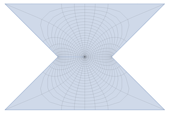
However, we have that

\frac{|T_{\delta}^{\prime\prime\prime}(0)|}{|T_{\delta}^{\prime}(0)|^{3}}=6\delta-2.

In particular we observe that for $\delta\in\Big{(}\frac{c_{0}+2}{6},1\Big{)}$ , $\nu=4$ satisfies (15). Since $0.9>\frac{c_{0}+2}{6}$ , the domain $\Omega_{0.9}$ is a suitable domain to do the construction of $\omega_{0}$ with $\nu=4$ . More details and illustrations about the family of domains $(\Omega_{\delta})_{\delta}$ are given in Appendix A.

To obtain a smooth domain $\widetilde{\Omega}_{d}$ with the same properties, one takes an increasing sequence $\Omega_{n}$ of smooth domains which are symmetric with respect to both axes and converge towards $\Omega_{9/10}$ . By symmetry, 0 is necessarily a critical point of the Robin’s function of every domain. Then, we introduce $T_{n}$ the sequence of conformal maps mapping $\Omega_{n}$ to $D(0,1)$ satisfying $T_{n}(0)=0$ and $T_{n}^{\prime}(0)\in\mathbb{R}_{+}$ . The construction can be done so that $T_{n}\to T_{9/10}$ locally in every $C^{k}$ , $k\geq 0$ , so that

\frac{|T_{n}^{\prime\prime\prime}(0)|}{|T_{n}^{\prime}(0)|^{3}}\underset{n\to+\infty}{\longrightarrow}\frac{|T_{9/10}^{\prime\prime\prime}(0)|}{|T_{n}^{\prime}(0)|^{3}}>c_{0},

so there exists $n_{0}\in\mathbb{N}$ , such that the smooth domain $\Omega_{n_{0}}$ is such that

4>\frac{\frac{5}{3}|T_{n_{0}}^{\prime\prime\prime}(0)|+2|T_{n_{0}}^{\prime}(0)|^{3}}{\sqrt{|T_{n_{0}}^{\prime\prime\prime}(0)|^{2}-4|T_{n_{0}}^{\prime}(0)|^{6}}}+1.

5.4 Proof of Theorem 2.8

Let $\delta\in\Big{(}\frac{c_{0}+2}{6},1\Big{)}$ , let $\Omega:=\Omega_{\delta}$ (or $\Omega_{n_{0}}$ as described in the previous section to work with a smooth domain), $z^{*}=0$ and $a=1$ .

From Sections 5.2 and 5.3, $\mathrm{D}f(0)$ has an eigenvalue $\lambda_{0}=\frac{1}{4\pi}\sqrt{12\delta(3\delta-2)}>0,$ so Hypothesis $(i)$ of Theorem 3.2 is satisfied. We recall that Hypothesis $(iii)$ is satisfied since $f$ and $F$ are Lipschitz maps far from the boundary.

Therefore, there only remains to prove that Hypothesis $(ii)$ is satisfied to apply Theorem 3.2 and conclude the proof of Theorem 2.8.

Let us compute.

	$\displaystyle\big{\|}F(B(t),t)-f(B(t))\big{\|}$	$\displaystyle=\left\|\int\nabla_{x}^{\perp}\gamma_{\Omega}(B(t),y)\omega(y,t)\mathrm{d}y-\frac{a}{2}\widetilde{\gamma}_{\Omega}(B(t))\right\|$
		$\displaystyle=\left\|\int\big{(}\nabla_{x}^{\perp}\gamma_{\Omega}(B(t),y)-(\nabla_{x}^{\perp}\gamma_{\Omega}(B(t),B(t))\big{)}\omega(y,t)\mathrm{d}y\right\|$
		$\displaystyle\leq C\|a\|\int\|y-B(t)\|\frac{\omega(y,t)}{a}\mathrm{d}y$
		$\displaystyle\leq C\sqrt{I(t)},$

where on the last line the constant $C$ depends only on $\Omega$ . Letting $\delta\to 1$ , we observe that $\lambda_{0}\to\frac{\sqrt{3}}{2\pi}$ . Now applying Theorem (3.2), we have that for any $\beta_{0}<1/2$ , one can construct a suitable $\omega_{0}$ satisfying (2) with $N=1$ and $\nu=4$ . Theorem 2.8 is now completely proved.

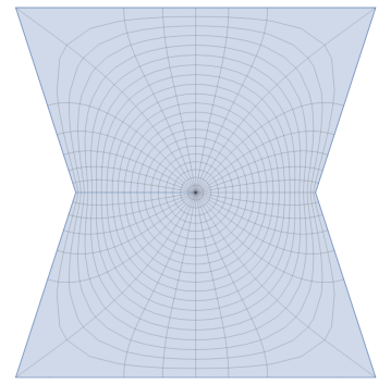
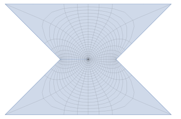
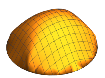
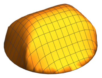
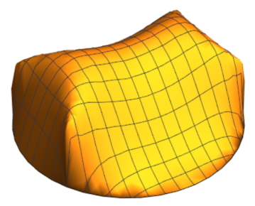
Appendix A The family of biconvex hexagonal domains and their Robin’s function

Let us mention that such domains were drawn and studied already in [11].

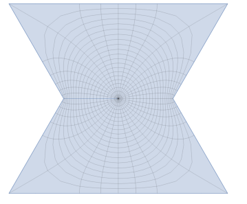
We used Wolfram Mathematica to plot several domains in Figure 2. In those cases, the Robin’s function is not a very nice function to plot. Instead we introduce the conformal radius:

r_{\Omega}(x)=e^{-2\pi\widetilde{\gamma}_{\Omega}(x)}.

It satisfies the transfer formula (see [11]):

r_{\Omega}(S(x))=|S^{\prime}(x)|r_{D}(x)=|S^{\prime}(x)|(1-|x|^{2}).

This map is a lot easier to draw, see Figure 3. We see that the Robin’s function of the domains obtained with $\delta>2/3$ have a saddle point in 0.

Appendix B Technical lemmas

B.1 Actual construction of the initial data

We formulate the following remark.

Remark B.1.

Let $N\geq 1$ , $Z^{*}\in(\mathbb{R}^{2})^{N}$ and $a_{i}\in\mathbb{R}^{*}$ . For any $Z_{0}$ such that $|Z_{0}-Z^{*}|=\frac{\varepsilon}{2}$ , one can always chose $\omega_{0}\in C^{\infty}(\mathbb{R}^{2})$ such that

•

$\omega_{0}$ satisfies (2),
•

$B(0)=Z_{0}$ ,
•

$\forall i\in\{1,\ldots,N\},\;I_{i}(0)\leq\varepsilon^{\nu}$ .

Proof.

For $N=1$ , $z_{0}\in\mathbb{R}^{2}$ , $a\in\mathbb{R}^{*}$ , we introduce the vortex patch $\omega_{0}=16a\frac{\varepsilon^{-\nu}}{\pi}\mathds{1}_{D(z_{0},\frac{\varepsilon^{\nu/2}}{4})}$ for $\varepsilon$ small enough. We verify that

|\omega_{0}|\leq C\varepsilon^{-\nu}

with $C=\frac{4a}{\pi}$ ,

\int\omega_{0}(x)\mathrm{d}x=a,

B(0)=\frac{1}{a}\int_{\mathbb{R}^{2}}x\omega_{0}(x)\mathrm{d}x=z_{0},

and

I(0)=\frac{1}{a}\int_{\mathbb{R}^{2}}|x-B(0)|^{2}\omega_{0}(x)\mathrm{d}x=\int_{0}^{\frac{\varepsilon^{\nu/2}}{4}}\int_{0}^{2\pi}16r^{2}\frac{\varepsilon^{-\nu}}{\pi}r\mathrm{d}\theta\mathrm{d}r=8\varepsilon^{-\nu}\frac{\varepsilon^{2\nu}}{256}=\frac{1}{32}\varepsilon^{\nu}.

For $N>1$ we sum patches of this exact form. One can also construct a smooth $\omega_{0}$ satisfying those constraints, by taking a convenient radially mollified version of these vortex patches such that their support lies within $D(z_{i},\varepsilon)$ . Since $\frac{\varepsilon^{\nu/2}}{4}<\varepsilon/2$ as $\nu\geq 2$ , it is always possible. ∎

B.2 Variant of the Gronwall’s inequality

From the Gronwall’s inequality, we can write the following.

Lemma B.2.

Let $f$ be a $C^{1}$ map and $g$ be positive non decreasing such that

|f(x)-f(y)|\leq\kappa|x-y|.

Let $z$ is a solution of

z^{\prime}(t)=f(z(t)),

and let $y$ such that

\begin{cases}\left|y^{\prime}(t)-f(y(t))\right|\leq g(t)\\ y(0)=z(0),\end{cases}

where $g:\mathbb{R}_{+}\to\mathbb{R}_{+}$ is smooth. Then

|y(t)-z(t)|\leq e^{\kappa t}\int_{0}^{t}g(s)\mathrm{d}s.

Proof.

On has that

	$\displaystyle\|y(t)-z(t)\|$	$\displaystyle=\left\|\int_{0}^{t}\big{(}y^{\prime}(s)+z^{\prime}(s)\big{)}\mathrm{d}s\right\|$
		$\displaystyle\leq\int_{0}^{t}g(s)\mathrm{d}s+\left\|\int_{0}^{t}\big{(}f(y(s))-f(z(s))\big{)}\mathrm{d}s\right\|$
		$\displaystyle\leq\int_{0}^{t}g(s)\mathrm{d}s+\kappa\int_{0}^{t}\|y(s)-z(s)\|\mathrm{d}s,$

so using now the classical Gronwall’s inequality, since $t\mapsto\int_{0}^{t}g(s)\mathrm{d}s$ is non decreasing, we have that

|y(t)-z(t)|\leq e^{\kappa t}\int_{0}^{t}g(s)\mathrm{d}s.

∎

Appendix C Computation of the constants

In Theorem 3.2, we proved that the construction is possible as long as

\nu>\frac{2}{5-\alpha}\left((1+\alpha)\frac{\kappa_{1}+\kappa_{2}}{\lambda_{0}}+4-2\alpha\right),

and

\xi_{1}>\frac{1-\beta}{\lambda_{0}}.

Since $\kappa_{1}$ , $\kappa_{2}$ and $\lambda_{0}$ ultimately depend on the chosen configuration of point-vortices, so do the bounds on $\nu$ and $\xi_{1}$ .

We now give details and improvements on those bounds.

C.1 Results

We state a few results that will be proved in the following sections.

By computing the constants $\kappa_{1}$ and $\kappa_{2}$ for the construction done in Section 4 with $N=3$ , we obtain the following details on the bound on $\nu$ .

Proposition C.1.

One can achieve the construction of Theorem 2.6 for any $\alpha\in[1,2)$ with any $\nu$ satisfying

\nu>\frac{2}{5-\alpha}\left((1+\alpha)\frac{2+2^{-\alpha}\alpha\sqrt{3(1+2^{1+2\alpha})}}{(2-2^{-\alpha})\sqrt{\alpha}}+4-2\alpha\right),

which is greater than $4$ .

Proposition C.2.

Let $\nu=4$ . There exists $\alpha_{0}>1$ such that for any $\alpha\in[1,\alpha_{0})$ , there exists an initial configuration $\big{(}(z_{i}^{*})_{i},(a_{i})_{i}\big{)}$ of point-vortices with $N=7$ and $\beta_{0}<\frac{4-2\alpha}{5-\alpha}$ such that for every $\beta\in(\beta_{0},1)$ there exists $\xi_{1}$ such that for every $\varepsilon>0$ small enough, there exists $\omega_{0}$ satisfying (2) such that any solution $\omega$ of (1) satisfies

\tau_{\varepsilon,\beta}\leq\xi_{1}|\ln\varepsilon|.

In particular, if $\alpha=1$ , one can take $\xi_{1}>\frac{4\pi}{9}(1-\beta)$ .

Unfortunately, we fail to obtain a rigorous estimate of $\alpha_{0}$ . However, in Section C.4, we numerically check that a construction using 9 blobs can be done with $\nu=4$ for any $\alpha\in[1,2)$ . The constant $\nu=4$ is not optimal.

C.2 How to compute the constants

We start by giving a general method on how to obtain $\kappa_{1}$ and $\kappa_{2}$ . Let $N\geq 3$ .

We recall that for all $t\leq\tau_{\varepsilon,\beta}$ , $\mathrm{supp}\hskip 2.84526pt\omega\subset\bigcup_{j=1}^{N}D(z_{j}^{*},\varepsilon^{\beta})$ . Therefore applying (16) to $\widetilde{z_{i}}=x$ , $\widetilde{x}=x^{\prime}-x$ , $\widetilde{z_{j}}=y$ , $\widetilde{y}=0$ , we have $\forall x,x^{\prime}\in D(z^{*},\varepsilon^{\beta})$ , and $\forall t\leq\tau_{\varepsilon,\beta}$ ,

	$\displaystyle F_{i}(x,t)-F_{i}(x^{\prime},t)$	$\displaystyle=\int\sum_{j\neq i}\big{(}K_{\alpha}(x,y)-K_{\alpha}(x^{\prime},y)\big{)}\omega_{j}(y,t)\mathrm{d}y$
		$\displaystyle=\sum_{j\neq i}C_{\alpha}\int\frac{(x-y)^{\perp}}{\|x-y\|^{\alpha+3}}(\alpha+1)(x^{\prime}-x)\cdot(x-y)\omega(y,t)\mathrm{d}y+o(\|x-x^{\prime}\|)$

so that

	$\displaystyle\Big{\|}(x-x^{\prime})\cdot\big{(}F_{i}(x,t)-F_{i}(x^{\prime},t)\big{)}\Big{\|}$	$\displaystyle\leq\|x-x^{\prime}\|^{2}\left(\sum_{j\neq i}\int\frac{C_{\alpha}}{\|x-y\|^{\alpha+1}}\|\omega(y,t)\|\mathrm{d}y+o(1)\right)$
		$\displaystyle\leq\|x-x^{\prime}\|^{2}\left(\sum_{j\neq i}\frac{C_{\alpha}\|a_{j}\|}{\|z_{i}^{}-z_{j}^{}\|^{\alpha+1}}+o(1)\right).$

Therefore we obtain that for every $i\in\{1,\ldots,N\}$ , for every $x,x^{\prime}\in D(z^{*},\varepsilon^{\beta})$ and for every $t\leq\tau_{\varepsilon,\beta}$ ,

\Big{|}(x-x^{\prime})\cdot\big{(}F_{i}(x,t)-F_{i}(x^{\prime},t)\big{)}\Big{|}\leq\kappa_{1}|x-x^{\prime}|^{2}

with

\kappa_{1}=C_{\alpha}\max_{1\leq i\leq N}\sum_{j\neq i}\frac{|a_{j}|}{|z_{i}^{*}-z_{j}^{*}|^{\alpha+1}}+o(1).

For $\kappa_{2}$ , we need a Lipschitz type estimate for $f$ on $\bigcup_{j=1}^{N}D(z_{j}^{*},2\varepsilon^{\beta})$ , and thus have that

\kappa_{2}=\Big{\|}{\left|\kern-1.07639pt\left|\kern-1.07639pt\left|\mathrm{D}f(Z)\right|\kern-1.07639pt\right|\kern-1.07639pt\right|}\Big{\|}_{\infty,\bigcup_{j=1}^{N}D(z_{j}^{*},2\varepsilon^{\beta})}={\left|\kern-1.07639pt\left|\kern-1.07639pt\left|\mathrm{D}f(Z^{*})\right|\kern-1.07639pt\right|\kern-1.07639pt\right|}+o(\varepsilon^{\beta})=\sqrt{\rho\big{(}\mathrm{D}f(Z^{*})[\mathrm{D}f(Z^{*})]^{t}\big{)}}+o(\varepsilon^{\beta})

where $\rho$ is the spectral radius, that is in our case the greatest eigenvalue in absolute value of the real symmetric matrix $\mathrm{D}f(Z^{*})[\mathrm{D}f(Z^{*})]^{t}$ .

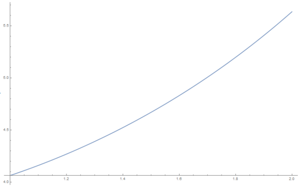
C.3 Proof of Proposition C.1

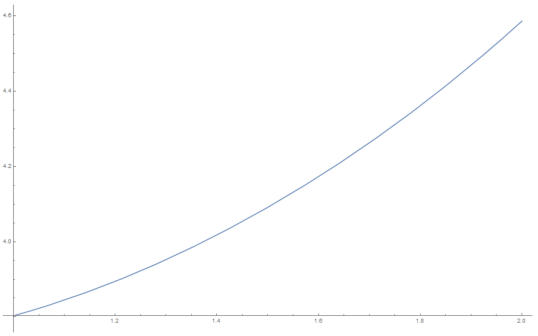
We now take again $N=3$ and compute. First, we directly have that

\kappa_{1}=2C_{\alpha}+o(1).

We now compute the eigenvalues of $\mathrm{D}f(Z^{*})[\mathrm{D}f(Z^{*})]^{t}$ and observe that

{\left|\kern-1.07639pt\left|\kern-1.07639pt\left|\mathrm{D}f(Z^{*})\right|\kern-1.07639pt\right|\kern-1.07639pt\right|}=C_{\alpha}2^{-\alpha}\alpha\sqrt{3(1+2^{1+2\alpha})}.

Therefore, it is possible to choose $\nu$ such that

\nu>\frac{2}{5-\alpha}\left((1+\alpha)\frac{\kappa_{1}+\kappa_{2}}{\lambda_{0}}+4-2\alpha\right)

for $\varepsilon$ small enough as soon as

\nu>\frac{2}{5-\alpha}\left((1+\alpha)\frac{2+2^{-\alpha}\alpha\sqrt{3(1+2^{1+2\alpha})}}{(2-2^{-\alpha})\sqrt{\alpha}}+4-2\alpha\right):=g(\alpha).

The plot of $\alpha\mapsto g(\alpha)$ is given in Figure 4. This concludes the proof of Proposition C.1.

C.4 Proof of Proposition C.2

Using the exact same method, we now construct the vortex crystal with $N=7$ .

Since $\forall i\neq j$ , $|z_{i}^{*}-z_{j}^{*}|\geq 1$ , then we obtain directly that one can take $\kappa_{1}=\frac{3}{\pi}+o(1)$ . However in general, we are not able to compute $\kappa_{2}$ and $\nu$ .

We now assume that $\alpha=1$ . We then compute that

\mathrm{D}f(Z^{*})=\frac{1}{2\pi}\times\\ {\footnotesize\left(\begin{array}[]{cccccccccccccc}c_{1}&-\frac{35}{24}&0&1&-\frac{1}{2\sqrt{3}}&\frac{1}{6}&-\frac{\sqrt{3}}{8}&-\frac{1}{8}&0&-\frac{1}{3}&\frac{\sqrt{3}}{2}&-\frac{1}{2}&\frac{5\sqrt{3}}{4}&\frac{5}{4}\\ -\frac{35}{24}&-c_{1}&1&0&\frac{1}{6}&\frac{1}{2\sqrt{3}}&-\frac{1}{8}&\frac{\sqrt{3}}{8}&-\frac{1}{3}&0&-\frac{1}{2}&-\frac{\sqrt{3}}{2}&\frac{5}{4}&-\frac{5\sqrt{3}}{4}\\ 0&1&-c_{1}&-\frac{35}{24}&-\frac{\sqrt{3}}{2}&-\frac{1}{2}&0&-\frac{1}{3}&\frac{\sqrt{3}}{8}&-\frac{1}{8}&\frac{1}{2\sqrt{3}}&\frac{1}{6}&-\frac{5\sqrt{3}}{4}&\frac{5}{4}\\ 1&0&-\frac{35}{24}&c_{1}&-\frac{1}{2}&\frac{\sqrt{3}}{2}&-\frac{1}{3}&0&-\frac{1}{8}&-\frac{\sqrt{3}}{8}&\frac{1}{6}&-\frac{1}{2\sqrt{3}}&\frac{5}{4}&\frac{5\sqrt{3}}{4}\\ -\frac{1}{2\sqrt{3}}&\frac{1}{6}&-\frac{\sqrt{3}}{2}&-\frac{1}{2}&0&\frac{35}{12}&\frac{\sqrt{3}}{2}&-\frac{1}{2}&\frac{1}{2\sqrt{3}}&\frac{1}{6}&0&\frac{1}{4}&0&-\frac{5}{2}\\ \frac{1}{6}&\frac{1}{2\sqrt{3}}&-\frac{1}{2}&\frac{\sqrt{3}}{2}&\frac{35}{12}&0&-\frac{1}{2}&-\frac{\sqrt{3}}{2}&\frac{1}{6}&-\frac{1}{2\sqrt{3}}&\frac{1}{4}&0&-\frac{5}{2}&0\\ -\frac{\sqrt{3}}{8}&-\frac{1}{8}&0&-\frac{1}{3}&\frac{\sqrt{3}}{2}&-\frac{1}{2}&c_{1}&-\frac{35}{24}&0&1&-\frac{1}{2\sqrt{3}}&\frac{1}{6}&\frac{5\sqrt{3}}{4}&\frac{5}{4}\\ -\frac{1}{8}&\frac{\sqrt{3}}{8}&-\frac{1}{3}&0&-\frac{1}{2}&-\frac{\sqrt{3}}{2}&-\frac{35}{24}&-c_{1}&1&0&\frac{1}{6}&\frac{1}{2\sqrt{3}}&\frac{5}{4}&-\frac{5\sqrt{3}}{4}\\ 0&-\frac{1}{3}&\frac{\sqrt{3}}{8}&-\frac{1}{8}&\frac{1}{2\sqrt{3}}&\frac{1}{6}&0&1&-c_{1}&-\frac{35}{24}&-\frac{\sqrt{3}}{2}&-\frac{1}{2}&-\frac{5\sqrt{3}}{4}&\frac{5}{4}\\ -\frac{1}{3}&0&-\frac{1}{8}&-\frac{\sqrt{3}}{8}&\frac{1}{6}&-\frac{1}{2\sqrt{3}}&1&0&-\frac{35}{24}&c_{1}&-\frac{1}{2}&\frac{\sqrt{3}}{2}&\frac{5}{4}&\frac{5\sqrt{3}}{4}\\ \frac{\sqrt{3}}{2}&-\frac{1}{2}&\frac{1}{2\sqrt{3}}&\frac{1}{6}&0&\frac{1}{4}&-\frac{1}{2\sqrt{3}}&\frac{1}{6}&-\frac{\sqrt{3}}{2}&-\frac{1}{2}&0&\frac{35}{12}&0&-\frac{5}{2}\\ -\frac{1}{2}&-\frac{\sqrt{3}}{2}&\frac{1}{6}&-\frac{1}{2\sqrt{3}}&\frac{1}{4}&0&\frac{1}{6}&\frac{1}{2\sqrt{3}}&-\frac{1}{2}&\frac{\sqrt{3}}{2}&\frac{35}{12}&0&-\frac{5}{2}&0\\ -\frac{\sqrt{3}}{2}&-\frac{1}{2}&\frac{\sqrt{3}}{2}&-\frac{1}{2}&0&1&-\frac{\sqrt{3}}{2}&-\frac{1}{2}&\frac{\sqrt{3}}{2}&-\frac{1}{2}&0&1&0&0\\ -\frac{1}{2}&\frac{\sqrt{3}}{2}&-\frac{1}{2}&-\frac{\sqrt{3}}{2}&1&0&-\frac{1}{2}&\frac{\sqrt{3}}{2}&-\frac{1}{2}&-\frac{\sqrt{3}}{2}&1&0&0&0\\ \end{array}\right)}

with $c_{1}=\frac{1}{2\sqrt{3}}-\frac{13\sqrt{3}}{8}$ .

Eigenvalues are $0$ (with multiplicity 4), $\pm i\frac{\sqrt{35}}{4\pi}$ (each with multiplicity 2), $\pm\frac{2}{\pi}$ (each with multiplicity 2) and $\pm\frac{9}{4\pi}$ , so on can let $\lambda_{0}=\frac{9}{4\pi}$ . Computations show that

\kappa_{2}=\sqrt{\rho\big{(}\mathrm{D}f(Z^{*})[\mathrm{D}f(Z^{*})]^{t}\big{)}}+o(1)=\frac{5\sqrt{7}}{2}+o(1).

Finally, it is easy to check that it is possible to choose $\nu$ such that relation (15) holds, for $\varepsilon$ small enough as soon as

\nu>\frac{12+5\sqrt{7}}{9}+1.

Observing that $\frac{12+5\sqrt{7}}{9}+1<4$ , we can conclude that we can construct $\omega_{0}$ satisfying (2) with $N=7$ and $\nu=4$ for $\alpha=1$ such that

\tau_{\varepsilon,\beta}\leq\xi_{1}|\ln\varepsilon|,

for any $\xi_{1}>4\pi\frac{1-\beta}{9}$ .

In order to conclude the proof of Proposition C.2, we observe that $a_{N}$ and thus $\frac{\kappa_{1}}{C_{\alpha}}$ , $\frac{1}{C_{\alpha}}\mathrm{D}f(Z^{*})$ and thus $\frac{\lambda_{0}}{C_{\alpha}}$ and $\frac{\kappa_{2}}{C_{\alpha}}$ are all depending continuously on $\alpha$ . Therefore, it holds true for $\varepsilon$ small enough that

\frac{2}{5-\alpha}\left((1+\alpha)\frac{\kappa_{1}+\kappa_{2}}{\lambda_{0}}+4-2\alpha\right)<4.

at least on a small interval $[1,\alpha_{0})$ . This ends the proof.

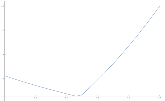
For a general value of $\alpha$ , the coefficients of the matrix $\mathrm{D}f(Z^{*})$ are too complicated to compute mathematically the eigenvalues. However, we use Wolfram Mathematica [18] to plot the map

h:\alpha\mapsto\frac{2}{5-\alpha}\left((1+\alpha)\frac{\displaystyle\max_{1\leq i\leq N}\sum_{j\neq i}\frac{|a_{j}|}{|z_{i}^{*}-z_{j}^{*}|^{\alpha+1}}+\sqrt{\max\big{|}\mathrm{Eigenvalues}\big{[}\mathrm{D}f(Z^{*})[\mathrm{D}f(Z^{*})]^{t}\big{]}\big{|}}}{\max\big{(}\operatorname{Re}(\mathrm{Eigenvalues}[\mathrm{D}f(Z^{*})]\big{)}}+4-2\alpha\right)

to obtain Figure 5, which shows that letting $N=9$ , we have that $\frac{2}{5-\alpha}\left((1+\alpha)\frac{\kappa_{1}+\kappa_{2}}{\lambda_{0}}+4-2\alpha\right)<4$ for every $\alpha\in[1,2)$ . Therefore, we have very strong numerical evidence of the fact that a construction is possible for every $\alpha\in[1,2)$ with $\nu<4$ (thus in particular with $\nu=4$ ). Please keep in mind that our method does not yield optimal constants. In particular, $\nu=4$ is not optimal.

Acknowledgments.

The author whishes to acknowledge useful discussions with Thierry Gallay, Pierre-Damien Thizy and Mickaël Nahon. This work was partly conducted when the author was working at the Université Claude Bernard Lyon 1, Institut Camille Jordan.

References

[1] H. Aref, P. K. Newton, M. A. Stremler, T. Tokieda, and D. L. Vainchtein. Vortex Crystals, volume 39 of Advances in Applied Mechanics. Elsevier, 2003.
[2] P. Buttà and C. Marchioro. Long time evolution of concentrated Euler flows with planar symmetry. SIAM J. Math. Anal., 50(1):735–760, 2018.
[3] H. E. Cabral and D. S. Schmidt. Stability of Relative Equilibria in the Problem of N+1 Vortices. SIAM Journal on Mathematical Analysis, 31(2):231–250, 2000.
[4] G. Cavallaro, R. Garra, and C. Marchioro. Localization and stability of active scalar flows. Riv. Mat. Univ. Parma 4, pages 175–196, 2013.
[5] G. Cavallaro, R. Garra, and C. Marchioro. Long time localization of modified surface quasi-geostrophic equations. Discrete & Continuous Dynamical Systems - B, 26(9):5135–5148, 2021.
[6] J. Davila, M. Del Pino, M. Musso, and J. Wei. Gluing Methods for Vortex Dynamics in Euler Flows. Archive for Rational Mechanics and Analysis, 235:1467–1530, 2020.
[7] M. Donati. Two-dimensional point vortex dynamics in bounded domains: Global existence for almost every initial data. SIAM Journal on Mathematical Analysis, 54(1):79–113, 2022.
[8] M. Donati and D. Iftimie. Long time confinement of vorticity around a stable stationary point vortex in a bounded planar domain. Annales de l’Institut Henri Poincaré C, Analyse non linéaire, 38(5):1461–1485, 2020.
[9] Tobin A. Driscoll and Lloyd N. Trefethen. Schwarz-Christoffel Mapping. Cambridge Monographs on Applied and Computational Mathematics. Cambridge University Press, 2002.
[10] D. Dürr and M. Pulvirenti. On the vortex flow in bounded domains. Communications in Mathematical Physics, pages 265–273, 1982.
[11] M. Flucher. Extremal functions for the trudinger-moser inequality in 2 dimensions. Commentarii mathematici Helvetici, 67(3):471–497, 1992.
[12] M. Flucher. Variational problems with concentration, volume 36 of Progress in Nonlinear Differential Equations and their Applications. Birkhäuser Verlag, Basel, 1999.
[13] C. Geldhauser and M. Romito. Point vortices for inviscid generalized surface quasi-geostrophic models. Am. Ins. Math. Sci., 25(7):2583–2606, 2020.
[14] L. Godard-Cadillac. Vortex collapses for the Euler and Quasi-Geostrophic models. Discrete and Continuous Dynamical Systems, 2022.
[15] L. Godard-Cadillac, P. Gravejat, and D. Smets. Co-rotating vortices with N fold symmetry for the inviscid surface quasi-geostrophic equation. Preprint, 2020. arXiv:2010.08194.
[16] B. Gustafsson. On the Motion of a Vortex in Two-dimensional Flow of an Ideal Fluid in Simply and Multiply Connected Domains. Trita-MAT-1979-7. Royal Institute of Technology, 1979.
[17] P. Hartman. Ordinary Differential Equations: Second Edition. Secaucus, New Jersey, U.S.A.: Birkhauser, 1982.
[18] Wolfram Research, Inc. Mathematica, Version 12.0. Champaign, IL, 2019.
[19] F. Marchand. Existence and regularity of weak solutions to the quasi-geostrophic equations in the spaces $L^{p}$ or $\dot{H}^{-1/2}$ . Comm. Math. Phys., 277(1):45–67, 2008.
[20] C. Marchioro and M. Pulvirenti. Vortex methods in two-dimensional fluid dynamics. Lecture notes in physics. Springer-Verlag, 1984.
[21] C. Marchioro and M. Pulvirenti. Mathematical Theory of Incompressible Nonviscous Fluids. Applied Mathematical Sciences. Springer New York, 1993.
[22] C. Marchioro and M. Pulvirenti. Vortices and localization in Euler flows. Comm. Math. Phys., 154(1):49–61, 1993.
[23] G. K. Morikawa and E. V. Swenson. Interacting Motion of Rectilinear Geostrophic Vortices. Physics of Fluids, 14(6):1058–1073, June 1971.
[24] J. Pedlosky. Geophysical Fluid Dynamics. Springer-Verlag, New-York, 1987.
[25] M. Rosenzweig. Justification of the point vortex approximation for modified surface quasi-geostrophic equations. Preprint, 2020. arXiv:1905.07351.
[26] D. Smets and J. Van Schaftingen. Desingularization of vortices for the Euler equation. Arch. Ration. Mech. Anal., 198(3):869–925, 2010.
[27] B. Turkington. On the evolution of a concentrated vortex in an ideal fluid. Archive for Rational Mechanics and Analysis, 97:75–87, 1987.
[28] G.K. Vallis. Atmospheric and Oceanic Fluid Dynamics. Cambridge University Press, 2006.
[29] V.I. Yudovich. Non-stationary flow of an ideal incompressible liquid. USSR Computational Mathematics and Mathematical Physics, 3(6):1407 – 1456, 1963.

	$\displaystyle\left\|\frac{\mathrm{d}}{\mathrm{d}t}B_{i}(t)-f_{i}(B(t))\right\|$	$\displaystyle=\left\|\frac{1}{a_{i}}\int\big{(}F_{i}(x,t)-f_{i}(B(t))\big{)}\omega_{i}(x,t)\mathrm{d}x\right\|$
		$\displaystyle=\left\|\frac{1}{a_{i}}\int\big{(}F_{i}(x,t)-F_{i}(B_{i}(t),t)+F_{i}(B_{i}(t),t)-f_{i}(B(t))\big{)}\omega_{i}(x,t)\mathrm{d}x\right\|$
		$\displaystyle\leq\kappa_{0}\int\|x-B_{i}(t)\|\frac{\omega_{i}(x,t)}{a_{i}}\mathrm{d}x+C\sum_{j=1}^{N}\sqrt{I_{j}(t)},$

	$\displaystyle\frac{1}{C_{\alpha}}$	$\displaystyle\big{(}K_{\alpha}(z_{i}+x,z_{j}+y)-K_{\alpha}(z_{i},z_{j})\big{)}$
		$\displaystyle=\frac{\big{(}(z_{i}+x)-(z_{j}+y)\big{)}^{\perp}}{\big{\|}(z_{i}+x)-(z_{j}+y)\big{\|}^{\alpha+1}}-\frac{(z_{i}-z_{j})^{\perp}}{\|z_{i}-z_{j}\|^{\alpha+1}}$
		$\displaystyle=\frac{(z_{i}-z_{j})^{\perp}}{\big{\|}(z_{i}+x)-(z_{j}+y)\big{\|}^{\alpha+1}}-\frac{(z_{i}-z_{j})^{\perp}}{\|z_{i}-z_{j}\|^{\alpha+1}}+\frac{(x-y)^{\perp}}{\big{\|}(z_{i}+x)-(z_{j}+y)\big{\|}^{\alpha+1}}$
		$\displaystyle=\frac{(z_{i}-z_{j})^{\perp}}{\|z_{i}-z_{j}\|^{\alpha+1}}\left(1-(\alpha+1)(x-y)\cdot\frac{z_{i}-z_{j}}{\|z_{i}-z_{j}\|^{2}}+o\big{(}\|x\|+\|y\|\big{)}-1\right)+\frac{(x-y)^{\perp}}{\|z_{i}-z_{j}\|^{\alpha+1}}+o\big{(}\|x\|+\|y\|\big{)},$

	$\displaystyle\left\|F_{i}(B_{i}(t),t)-f_{i}(B(t))\right\|$	$\displaystyle=\left\|\sum_{j\neq i}\int K_{\alpha}(B_{i}(t),y)\omega_{j}(y,t)\mathrm{d}y-\sum_{j\neq i}a_{j}K_{\alpha}(B_{i}(t),B_{j}(t))\right\|$
		$\displaystyle=\left\|\sum_{j\neq i}\int\big{(}K_{\alpha}(B_{i}(t),y)-K_{\alpha}(B_{i}(t),B_{j}(t))\big{)}\omega_{j}(y,t)\mathrm{d}y\right\|$
		$\displaystyle\leq\sum_{j\neq i}\int\big{\|}K_{\alpha}(B_{i}(t),y)-K_{\alpha}(B_{i}(t),B_{j}(t))\big{\|}\frac{\|a_{j}\|\omega_{j}(y,t)}{a_{j}}\mathrm{d}y$
		$\displaystyle\leq C\sum_{j\neq i}\|a_{j}\|\int\big{\|}y-B_{j}(t)\big{\|}\frac{\omega_{j}(y,t)}{a_{j}}\mathrm{d}y$
		$\displaystyle\leq C\sum_{j\neq i}\sqrt{I_{j}(t)},$

	$\displaystyle\big{\|}F(B(t),t)-f(B(t))\big{\|}$	$\displaystyle=\left\|\int\nabla_{x}^{\perp}\gamma_{\Omega}(B(t),y)\omega(y,t)\mathrm{d}y-\frac{a}{2}\widetilde{\gamma}_{\Omega}(B(t))\right\|$
		$\displaystyle=\left\|\int\big{(}\nabla_{x}^{\perp}\gamma_{\Omega}(B(t),y)-(\nabla_{x}^{\perp}\gamma_{\Omega}(B(t),B(t))\big{)}\omega(y,t)\mathrm{d}y\right\|$
		$\displaystyle\leq C\|a\|\int\|y-B(t)\|\frac{\omega(y,t)}{a}\mathrm{d}y$
		$\displaystyle\leq C\sqrt{I(t)},$

	$\displaystyle\|y(t)-z(t)\|$	$\displaystyle=\left\|\int_{0}^{t}\big{(}y^{\prime}(s)+z^{\prime}(s)\big{)}\mathrm{d}s\right\|$
		$\displaystyle\leq\int_{0}^{t}g(s)\mathrm{d}s+\left\|\int_{0}^{t}\big{(}f(y(s))-f(z(s))\big{)}\mathrm{d}s\right\|$
		$\displaystyle\leq\int_{0}^{t}g(s)\mathrm{d}s+\kappa\int_{0}^{t}\|y(s)-z(s)\|\mathrm{d}s,$