Constraining the oblateness of transiting planets with photometry and spectroscopy
Abstract
Rapid planetary rotation can cause the equilibrium shape of a planet to be oblate. While planetary oblateness has mostly been probed by examining the subtle ingress and egress features in photometric transit light curves, we investigate the effect of oblateness on the spectroscopic Rossiter-McLaughlin (RM) signals. We found that a giant planet, with planet-to-star radius ratio of 0.15 and Saturn-like oblateness of 0.098, can cause spectroscopic signatures with amplitudes up to 1.1 m s-1 which is detectable by high-precision spectrographs such as ESPRESSO. We also found that the spectroscopic oblateness signals are particularly amplified for transits across rapidly rotating stars and for planets with spin-orbit misalignment thereby making them more prominent than the photometric signals at some transit orientations. We compared the detectability of oblateness in photometry and spectroscopy and found that photometric light curves are more sensitive to detecting oblateness than the spectroscopic RM signals mostly because they can be sampled with higher cadence to better probe the oblateness ingress and egress anomaly. However, joint analyses of the light curve and RM signal of a transiting planet provides more accurate and precise estimate of the planet’s oblateness. Therefore, ESPRESSO alongside ongoing and upcoming photometric instruments such as TESS, CHEOPS, PLATO and JWST will be extremely useful in measuring planet oblateness.
keywords:
Planets and satellites - techniques: photometric, spectroscopic1 Introduction
Planets have non-spherical equilibrium shapes as a result of different forces acting upon them such as gravitational, pressure, tidal and centrifugal forces. The centrifugal acceleration caused by planetary rotation reduces the effective gravitational acceleration at the equator compared to the pole thereby leading to an equatorial bulge. The resulting non-spherical planet shape is referred to as oblateness (Seager & Hui, 2002) and is defined by an oblateness parameter, , given as (e.g., Barnes & Fortney 2003; Carter & Winn 2010a)
| (1) |
where and represent the equatorial and polar radii of the planet respectively.
Knowledge of the oblateness of a planet can provide information about its rotation rate (or rotation period) and internal density structure. These can in turn shed valuable insight into the planet’s formation and evolution (Lissauer, 1995; Li & Lai, 2020), as well as its atmospheric circulation and dynamics (Kaspi & Showman, 2015). The solar system planets have different rotation periods and oblateness indicating diverse formation and evolutionary histories (Laskar & Robutel, 1993). Saturn, having one of the fastest rotation with a period of only 10.7 hrs, has the highest oblateness of (i.e., its polar radius is 9.8% smaller than its equatorial radius). Although Saturn rotates slightly slower than Jupiter, it has a significantly lower density, and thus less gravity, which allows its rotation induce a higher oblateness than in Jupiter (with ).
Measuring the oblateness of exoplanets is challenging as the induced effects in transit signals have low amplitudes. Previous studies investigated the photometric difference between the transit light curve of an oblate planet and the corresponding spherical planet (e.g Seager & Hui 2002; Barnes & Fortney 2003; Carter & Winn 2010a). They showed that the amplitude of the oblateness-induced signal for a giant planet, with Saturn-like oblateness and planet-to-star radius ratio of 0.1, is just around 100 ppm for the best case transit geometry. Zhu et al. (2014) searched for oblateness signals in Kepler light curve data and obtained a tentatively high oblateness of 0.22 for the brown dwarf Kepler-39b although they could not validate the consistency of the measurement across different subsets of the data. Later work by Biersteker & Schlichting (2017) did not detect the oblateness of Kepler-39b but put loose constraints on the oblateness of Kepler-427b. Therefore, measuring the oblateness of planets remains challenging. For very precise transit signals, assuming sphericity for an oblate planet would lead to systematic errors in the determination of the transit parameters (Barnes & Fortney, 2003).
In this paper, we complement the previous works by investigating, for the first time, the signature of planet oblateness in transit spectroscopy using the Rossiter-McLaughlin (RM) effect - the radial velocity (RV) anomaly caused by a companion transiting a rotating star (Rossiter, 1924; McLaughlin, 1924). Besides the usual planetary transit parameters, the RV anomaly caused by a planet additionally depends on the projected stellar rotation velocity, , and the projected spin-orbit angle, , between the sky projections of the stellar spin axis and the planetary orbit normal (Gaudi & Winn, 2007). We compare the detectability of oblateness from spectroscopic RM signals to that from photometric light curves and also the prospects of combining both measurements for a more precise measurement of oblateness.
In Sect. 2, we describe the oblate planet model and transit tool used in generating oblate planet light curves and RM signals. We used the tool to confirm photometric results from previous studies while showing also the expected spectroscopic result. In Sect. 3, we identify the optimal parameter space for detecting the photometric and spectroscopic oblateness signal and also investigate the detectability of oblateness considering different observing instruments. In Sect. 4, we discuss the results and conclude in Sect. 5.
2 Oblate planet transit
As mentioned in Barnes & Fortney (2004) and Akinsanmi et al. (2018), the projected shape of a planet with a continuous opaque ring extending directly from the planet surface (so that there is no gap between them) will mimic the projected shape of an oblate planet; if the ring is appropriately inclined with respect to the sky plane. As such, a ringed planet model can be used to simulate the expected photometric light curve and spectroscopic RM signal of an oblate planet. Therefore, we employ the SOAP3.0 ringed planet tool (Akinsanmi et al., 2018) to model the transit of an oblate planet111Although there might be some slight differences in using a ringed planet model to emulate the projected shape of oblate planets, it serves as a sufficient approximation and produces desired results consistent with previous studies.. The ring is defined by four parameters: the inner and outer ring radii, and , in units of a core planetary radius , and also two orientation angles and which define the inclination of ring plane with respect to the sky plane and the obliquity of ring from the orbital plane, respectively (see Fig. 1 in Akinsanmi et al. 2018).
As depicted in Fig. 1, the projected shape of an oblate planet can be obtained using the ring planet model by first setting a core planet with a negligibly small radius (e.g. 10% of the required ; this is necessary since the inner and outer ring radii are in units of a core planet). A circular opaque ring starting at the surface of the core planet is then added with outer radius extending out to the equatorial radius of the oblate planet to be modeled. Oblateness of the entire projected figure (core planet + ring) can be obtained by inclining the ring away from sky plane by which imitates a reduced radius at the poles compared to the equator. As increases, the total projected figure becomes more oblate ( increases). The obliquity of the ring also corresponds to the obliquity of the oblate planet defining the projected angle between its equatorial plane and the orbital plane. It ranges from to with positive angles measured anti-clockwise from the transit chord and negative angles measured clockwise.

The rotation period () of the planet is related to the oblateness () by
| (2) |
where and represent the quadrupole moment and mass of the planet, respectively (Carter & Winn, 2010a). This equation shows that is inversely proportional to the rotation period and density () of the planet, so the effect of oblateness will be most significant for gaseous planets with short rotation periods.
We point out that and measured from transit light curves are not the true planet oblateness and obliquity but their projection on the sky plane since they are derived from the projected shape of the transiting planet (an ellipse). This means that the transit-derived values of and will always be lower limits on the true values. This, in turn, implies that only an upper limit on can be obtained (Seager & Hui, 2002; Carter & Winn, 2010a).
We define the mean radius of an oblate planet by
| (3) |
So for , and the mean radius of the oblate planet is same as the radius of a spherical planet. The maximum possible value of that can be attained by a planet is at the rotational break-up limit when the centrifugal acceleration balances the gravitational acceleration at the equator and this is at (Carter & Winn, 2010a).
2.1 Oblateness-induced signal in light curves and RM signals
Previous studies compared the transit light curve of an oblate planet to that of a spherical planet and showed that the oblateness signal manifests itself at the ingress and egress phases (e.g., Carter & Winn 2010a; Zhu et al. 2014). The oblateness-induced signal is a geometrical effect and is obtained as the residuals from fitting the transit observation of an oblate planet with a spherical planet model. The signal arises mostly due to difference in contact times at the stellar limb (ingress and egress) between the transiting oblate planet and the corresponding spherical planet of the same area. Since the geometry of a transiting planet is the same when taking photometric and spectroscopic transit measurements, the oblateness signature should also manifest itself in the transit RM signal.
To illustrate the oblateness signature in the light curve and RM signal, we follow the work of Carter & Winn (2010a) which analysed seven Spitzer transit observations of the giant planet HD 189733b to constrain its oblateness. The planet was selected due to its large size, bright host star and availability of precise Spitzer data. First, they calculated the theoretical oblateness signal amplitude expected for HD 189733b by simulating its photometric light curve assuming Saturn-like oblateness of and projected obliquity . The planet has the following parameters: planet-star mean radius ratio (equivalent to ), scaled semi-major axis , inclination (or impact parameter ) and orbital period days (Torres et al., 2008). The host star is of K2 spectral type with V-magnitude = 7.7, radius and km s-1 but we assume a stellar inclination (rotation axis parallel to sky plane). We also simulated mock oblate planet transit signals (light curve and RM signal) for this planet using SOAP3.0. The light curve was generated with Spitzer cadence of 2 minutes using quadratic limb darkening coefficients (LDCs) of [0.076, 0.034] in the Spitzer infrared band as given in Carter & Winn (2010a). The RM signal was generated with an integration time of 4 mins222 This integration time is similar to the 5 mins exposures of HARPS archival RM observations of HD 189733b used by Triaud et al. 2009; Wyttenbach et al. 2015. which, for real observations, will help reduce the amplitude of stellar noise in this star as recommended in Chaplin et al. (2019) for K-dwarfs. We obtained LDCs for the star in the visible band using Claret & Bloemen (2011) and assumed (close to the value of derived in Triaud et al. 2009). We then separately fit the oblate planet light curve and also its RM signal with spherical planet models. The residuals (oblate - spherical) from both fits are shown in Figure 2 with their amplitudes () quoted. The residuals show the effects of oblateness at ingress and egress as described in Seager & Hui (2002) and Barnes & Fortney (2003).

The residuals from our light curve fit is in agreement, in shape and amplitude, with the photometric result obtained in Carter & Winn (2010a) for this planet (see their Figure 1). The oblateness-induced signature in the RM signal, shown here for the first time, has an amplitude m s-1 whereas the ESPRESSO spectrograph (installed on the 8m class telescopes of the ESO VLT; Pepe et al. 2014) is capable of attaining instrumental RV precisions up to 0.1 m s-1. Using the ESPRESSO Exposure Time Calculator (ETC)333www.eso.org/observing/etc - Version P105.6, we estimated that the theoretical ESPRESSO RV precision for this star for the 4-minute exposure time is 0.31 m s-1 for observation in the high resolution (UT1; 140,000) mode444Note: In simulating the aforementioned RM signal, we used this ESPRESSO resolution to calculate the FWHM of the CCF which was additionally broadened to account for macro-turbulence (convection) using calibration equation from Doyle et al. (2014).. Taking into account the rotational velocity broadening which degrades the quality factor of the spectra with respect to its non-rotating counterpart, the RV precision for this star degrades by a factor of 1.8 to 0.56 m s-1 (calculated by interpolating between values in Table 2 of Bouchy et al. 2001). This precision can still be better if data is phase folded over an increased number of transit observations (n) as it scales in the photon noise limit with . If we assume that seven transits are observed (number of Spitzer transits analysed in Carter & Winn 2010a), a better RV precision of 0.2 m s-1 would be achieved which is much lower than the spectroscopic oblateness amplitude of this system. Moreover, RM measurements of longer period planets can be obtained with longer exposure times that provide a higher RV precision such that several transit observations are not necessarily needed.
Although the analysis of this system is simply illustrative, it hints that ESPRESSO RM measurements of "relevant" systems with transiting planets could allow reasonable constraints to be placed on planet oblateness in addition to those from light curve analysis. We further investigate this possibility in the following sections with suitable considerations.
We point out that the oblateness signal can be similar to the signal caused by the presence of rings (Seager & Hui, 2002; Barnes & Fortney, 2004). However, depending on ring orientation and size of the gap between the planet and ring, the ring signature can be distinct showing more peaks at ingress and egress than the oblateness signature (see Ohta et al. 2009; Akinsanmi et al. 2018). Additionally, an estimate of the planetary density can help distinguish them since a planet with rings will appear larger and cause the planetary density to be underestimated (Zuluaga et al., 2015; Akinsanmi et al., 2020).
2.2 Tidal interaction
In the previous section we showed the signature of oblateness in the photometric light curve and spectroscopic RM signal for a short period planet. However, short period planets such as HD 189733b have short tidal evolution timescales so they are expected to already have circularized orbits and synchronised rotations such that becomes equal to (Guillot et al., 1996). Such short period planets cannot have significant rotation induced oblateness since their rotations will be too slow (Seager & Hui, 2002). Indeed, Carter & Winn (2010a) did not detect oblateness in this planet for this same reason inspite of the large theoretically expected photometric signal (top panel of Fig. 2). However, short period planets can still be radially deformed (in direction of the star) due to the strong stellar tidal interaction. Previous studies (e.g. Correia 2014; Akinsanmi et al. 2019; Hellard et al. 2019) discussed the detectability of tidally induced deformation in short period planets and showed that this deformation diminishes with distance to the star.
Strong tidal interaction also affects the obliquity of short period planets by driving the value of to zero at the same short timescale for attaining rotation synchronization (Peale, 1999). Avoiding stellar tidal interaction then imposes the requirement for long period orbits to ensure rapid planet rotation for significant oblateness. Seager & Hui (2002) and Carter & Winn (2010b) showed that a Jupiter-mass planet orbiting a Solar twin star at a distance of 0.2 AU ( days) will have tidal synchronization timescale of 10 Gyrs (which is greater than the age of most host stars) so that the planet is not expected to have spun down and can therefore have significant rotation.
2.3 Spin precession
The spin axis of an oblate planet will precess due to the gravitational torque exerted on the planet by the host star. The effect of spin precession on transit signals is that the orientation of the oblate planet changes with time and so does its projection. This leads to transit depth variations between obtained light curves and amplitude variations between the RM signals. Such variations can complicate efforts to measure the ingress and egress oblateness signature since combining successive transits might average out the subtle signal. However, a Jupiter or Saturn-like planet with days is expected to have precession period of 50 yrs (Carter & Winn, 2010b) which is too long to be observed within a few transit observations of the planet. For example, the spin axis of a days planet will precess by a negligible in 3 successive transit observations thereby allowing the phase folding of data to probe oblateness.
Although some studies (e.g. Carter & Winn 2010b; Biersteker & Schlichting 2017) have illustrated the possibility of detecting oblateness due to spin precession for days, we investigate here the case of planets with days for which significant rotation induced oblateness is expected and spin precession is negligible.
| Parameter [Unit] | Value |
|---|---|
| 0.1546 | |
| 70.75 | |
| [days] | 50.0 |
| 0.0 | |
| 0.0980 | |
| Stellar type | K2V |
| 7.7 | |
| , | 0.5151, 0.3872 |
| [km s-1] | 5.0 |
3 Detecting oblateness
3.1 Identifying optimal transit geometry for detecting oblateness
As the oblateness signal can depend strongly on the projected orientation of the planet () and that of its orbit ( or ), it is important to identify the combinations of these two parameters that are optimal for detecting oblateness. Even though the value of is unknown a-priori for planets, an understanding of how it affects the detectability of oblateness is crucial as it can be used to calculate the maximum theoretical oblateness signal expected for a planet and thus aid in target selection. Although previous works (e.g., Barnes & Fortney 2003; Zhu et al. 2014) have identified parameter combinations with the highest photometric oblateness signal amplitude, we are particularly interested in understanding how the spectroscopic signal amplitude varies in comparison to the precision of new spectrographs like ESPRESSO.
We take case study of the HD189733 system assuming its Jupiter-sized planet () has a circular orbit around the star with a longer period of 50 days (based on requirements from previous section). As in the previous section, we assume a projected planet oblateness of . We also assume that the star rotates slightly faster with km s-1 (taking ). We use quadratic LDCs for this star in the visual band obtained from Claret & Bloemen (2011) but re-parameterized as [, ] following Kipping (2013). The full adopted parameters for the simulated system is given in Table 1.
We used SOAP3.0 to generate theoretical transit signals (light curves and RM signals) for the adopted oblate planet on a grid of obliquity () and impact parameter () values with a total of 42 combinations (excluding grazing transits since their ingress/egress are undefined). The transit durations and ingress (egress) durations of the transit signals vary with . From = 0 to = 0.8, the transit durations decrease from 6.3 hrs to 4.5 hrs whereas the ingress (egress) durations increase from 55 mins to 90 mins. Transits at higher impact parameters will thus allow better sampling of oblateness induced features due to their longer ingress and egress durations. The light curves were simulated with 2-min integration time (or binning) similar to TESS but applicable to other photometric instruments to increase the attained precision of each measurement. The RM signals had a longer integration time of 8 mins555 Spectroscopic transit observations usually require longer integrations than the photometric because spectrographs lose photons due to slit losses, stray light, and scattered light and so require longer time to collect more photons (Oshagh, 2018a). Long integrations are also used to average out and reduce stellar RV noise. We note also that longer period planets can have longer integrations which should be chosen such that the ingress and egress are still well sampled. which enables ESPRESSO reach a higher RV precision of 0.22 m s-1 while still providing good temporal resolution of the ingress and egress of this planet. Other spectrographs (like HARPS installed on a smaller 3.6 m telescope) are not capable of reaching such precision within this short integration time. To attain the same precision as ESPRESSO, HARPS will require 30 mins integrations which will not allow enough data points to probe oblateness signatures at ingress and egress.
We perform a least squares fit to the oblate planet light curve and RM signal of each parameter combination using a spherical planet model and obtain the amplitude, , of the residuals (at ingress/egress). The free parameters in the light curve fit were , , , , and, while the RM signal fit additionally had and .

Figure 3 shows the contour plots generated using the residual amplitudes from fitting the photometric light curve and spectroscopic RM signal of each parameter combination. It represents the amplitude of observable oblateness-induced signal, , at each parameter combination. The contours are shown only for positive angles as the pattern is symmetric about . In both contour plots, we see a similar trend showing that the amplitude of photometric and spectroscopic oblateness signal is lowest (yellow regions) at zero obliquity across all impact parameters. This implies that the best-fit spherical model can easily emulate the light curve and RM signal of the oblate planet by adjusting its fit parameters thereby making it difficult to detect oblateness at these orientations. However, at higher obliquities, the amplitude increases with impact parameter due to asymmetry between ingress and egress of the oblate planet transit signal that cannot be easily emulated by a spherical model. The oblateness signal reaches its peak amplitude at points around , (dark blue regions) in agreement with the results of earlier photometric studies (e.g. Seager & Hui 2002; Carter & Winn 2010a) but confirmed here to be same in spectroscopy. The contour plot is nearly symmetric about the vertical line with the exception of a few orientations around .
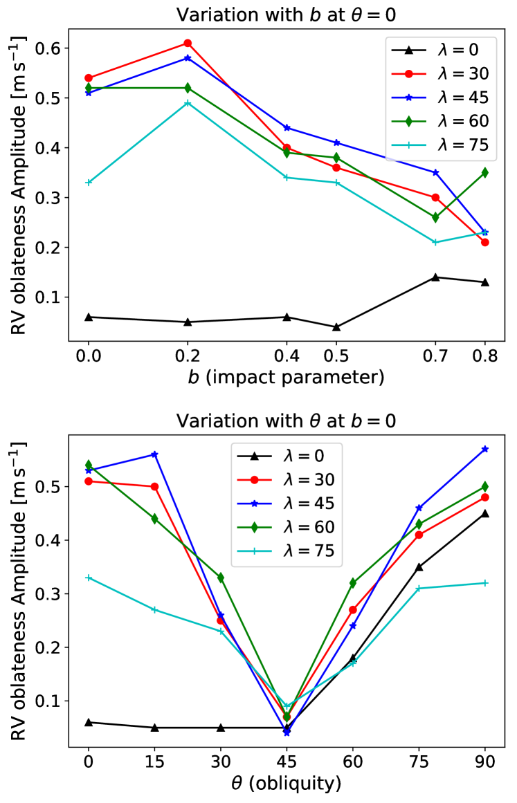
We also investigated how the spin-orbit angle () affects the amplitude of oblateness signal. For the yellow regions in Fig. 3 with low oblateness signal amplitudes (e.g. orientations with and those with ), we find that the spectroscopic oblateness signal amplitudes can increase for planets with spin-orbit misalignment (i.e. 0). For example, the spectroscopic oblateness amplitude at the orientation = , = 0.2 is only 0.05 m s-1 when but significantly increases to 0.61 m s-1 for . In contrast, this orientation has a photometric oblateness amplitude of only 3 ppm irrespective of . The orientations in the yellow regions can thus be more favorable for detecting oblateness in spectroscopy than in photometry. Figure 8 shows the variation of the spectroscopic oblateness amplitude with at orientations with and also orientations with .

In summary, Fig. 3 shows that the oblateness-induced signal is more prominent, in photometry and spectroscopy, for oblique planets at high impact parameters particularly for the points around , (optimal transit orientation) which provides the best opportunity to measure oblateness. The residual from the fit of this orientation is shown in Fig. 4 with photometric and spectroscopic oblateness amplitudes of 272 ppm and 1.1 m s-1, respectively.
The amplitude of the photometric and spectroscopic oblateness-induced signal for a particular parameter combination () scales with the oblateness and planet radius as (Barnes & Fortney, 2003). Therefore, planets with larger planet-to-star radius ratios will have larger oblateness signatures for the same projected oblateness. For the same planet, the spectroscopic oblateness amplitude () additionally scales with the projected stellar rotational velocity following the relation
| (4) |
3.2 Oblateness detectability
Detecting planet oblateness implies obtaining a measurement for the parameter by fitting a transit observation, of sufficient precision, with an oblate planet model. Recovering implies that a spherical planet model is a better fit to the observation than an oblate planet model. Detecting oblateness thus requires that is recovered with accuracy and statistical significance above zero from the fitting process.
To illustrate the photometric and spectroscopic detectability of oblateness, we simulated the transit signals (light curve and RM) of the oblate planet at the determined optimal orientation (Table 1 with ) which have oblateness amplitudes of 272 ppm and 1.1 m s-1 (Fig. 4). The light curve and RM signal were simulated with cadences of 2 mins and 8 mins, respectively. Random Gaussian (white) noise of different levels, , was added to the simulated transit signals. We then investigated how well we can recover and at what noise level it would be difficult to distinguish between the oblate planet and spherical planet transit signals (light curve and RM). This is useful in order to understand the instrumental precisions required for photometric and spectroscopic detection of oblateness.
We performed a Markov Chain Monte Carlo (MCMC) analysis with SOAP3.0 model to recover the oblate planet transit parameters along with their uncertainties. We use the emcee package (Foreman-Mackey et al., 2013) with priors on the parameters as given in Table. 2. We assume that the LDCs can be known with 10% accuracy so we adopt gaussian priors on them centered on the true simulated values with 10% standard deviation. The MCMC was performed with 36 walkers each having 20,000 steps (which was several times the computed auto-correlation time as recommended in emcee as a convergence diagnostic). The initial 25% of the steps were then discarded as burn-in.
Figure 5 shows the oblateness detectability plot, in photometry and spectroscopy, indicating the median and standard deviations of the recovered at different noise levels (average of three MCMC realizations). For oblateness to be confidently detected ( measured), we require that is recovered with significance above zero.666 As a check of our MCMC analysis, we confirmed that fitting a spherical planet transit signal with an oblate planet model recovers at different noise levels. We see in the spectroscopic detectability plot (right panel of Fig. 5) that is detected with significance for noise levels up to 1 m s-1/8 mins. At higher noise levels, the distribution of the recovered samples include at implying that a spherical planet model is also probable. In the photometric detectability plot (left panel of Fig. 5), a detection is attained for noise levels up to 400 ppm/2 mins. We note that detection of oblateness can still be attained at higher noise levels (up to 550 ppm in photometry and 1.5 m s-1 in spectroscopy).
| Parameter | Prior | Interval |
|---|---|---|
| Uniform | ||
| Uniform | ||
| Uniform | ||
| Gaussian | ||
| Gaussian | ||
| Uniform | ||
| Uniform | ||
| Uniform | ||
| Gaussian |


Figure 6 shows realized posterior distributions of the retrieved parameters at the detectable noise limits (400 ppm noise added to light curve and 1 m s-1 added to RM signal). In both cases, we see from the joint distributions that is not well-constrained and is strongly correlated with ( is only better constrained for highly precise transit signals). Figure 3 already showed that the amplitude of the oblateness signal is fairly symmetric about and reduces as the value of gets farther from . Therefore, for values different from in the distribution, the amplitude of oblateness signal reduces and a higher value of is needed to fit the observation. The degeneracy between and is responsible for the long tail towards large oblateness in the distribution (also seen for all noise levels in Fig. 5).
We converted the posterior of the fitted mean radius to using equation 3 to show the evidently strong correlation between and ; as the oblateness increases, the equatorial radius gets more elongated compared to the polar radius. It is interesting to see that the limb darkening parameters (, ) are not strongly correlated with implying that very precise determination of the LDCs are not required to detect planetary oblateness which is contrary to the case for detecting rings (Akinsanmi et al., 2018). Indeed when we adopt a non-informative uniform prior of on the LDCs, is still similarly recovered but with larger uncertainties on the LDCs and on the other parameters. The posteriors from the RM signal MCMC (left panel in Fig. 6) also shows that and are not correlated with implying that planetary oblateness does not affect the accurate retrieval of these parameters from RM signals.
We investigated also the retrieval of from combined analysis of the photometric light curve and spectroscopic RM signal. As seen in Fig. 5, is not recovered with for noise levels of 450 ppm (added to the light curve) and 1.2 m s-1 (added to the RM signal). However, simultaneously fitting both transit signals allows the recovery of with significance and with better accuracy as shown in Fig. 7 (compared to the Figs. 5 and 6).
| Instrument | Noise/time | Noise/time |
|---|---|---|
| @ | @ | |
| TESS a | 512 ppm/2 mins | 1109 ppm/2 mins |
| CHEOPS b | 127 ppm/2 mins | 219 ppm/2 mins |
| PLATO c | 44 ppm/2 mins | 148 ppm/2 mins |
| JWST (NIRCam) d | 40 ppm/2 min | 72 ppm/2 mins |
| ESPRESSO e | 0.25 m s-1/8 mins | 0.65 m s-1/8 mins |
| (@=5 km s-1)∗ | (0.58 m s-1/8 mins ) | (1.5 m s-1/8 mins) |
a heasarc.gsfc.nasa.gov/cgi-bin/tess/webtess/wtv.py
b cheops.unige.ch/pht2/exposure-time-calculator
c Rauer et al. (2014)
d Noise floor from Beichman
et al. (2014). Also noise estimate from (Hellard et al., 2019).
e www.eso.org/observing/etc. ∗ The RV noise level increases by a factor of 2.3 for = 5 km s-1 (Bouchy
et al., 2001).
4 DISCUSSION
As shown in Fig. 5, white noise levels of 400 ppm in photometry and 1 m s-1 in spectroscopy are the detectability noise limits required to measure Saturn-like oblateness in our hypothetical HD189733b-like planet (Table 1). We compare these detectability limits with the noise level attainable by different observing instruments for stars of different magnitudes as given in Table 3. The theoretical ESPRESSO noise levels for and stars after considering the effect of stellar rotation are 0.58 m s-1 and 1.5 m s-1 per 8 min integrations respectively. The spectroscopic detectability noise limit of 1 m s-1 is only attainable for stars which implies that ESPRESSO is capable detecting the oblateness of planets mostly around bright stars (). For stars of , ESPRESSO can still constrain the oblateness but with a lesser significance (). In contrast, the photometric detectability noise level of 400 ppm/2min is well attainable by CHEOPS, PLATO and JWST for oblateness detection for planets transiting stars as faint as . TESS is only capable of measuring for the brightest stars () and with significance.
In general, we define as the ratio of the expected oblateness signal amplitude to the observational noise level which can be used to set a baseline for detecting oblateness. A detection of Saturn-like oblateness for our hypothetical planet thus requires (i.e. 272 ppm/400 ppm) for photometry and (i.e. 1.1 m s-1/1 m s-1) for spectroscopy. However, a detection only requires of 0.5 and 0.73 for photometry and spectroscopy, respectively. Therefore, for a planet of with photometric and spectroscopic of 103 ppm and 0.42 m s-1 respectively, a detection of oblateness will require noise level, , below 103/0.5 = 206 ppm in the photometric light curve and below 0.42/0.73 = 0.58 m s-1 in spectroscopic RM signal. Comparing with Table 3, the required noise level can be attained by CHEOPS for , by PLATO and JWST for even fainter stars and by ESPRESSO for stars with . However, noise levels can be lowered to favour more significant detection if several transits are combined.

We found that the photometric data is more sensitive for detecting oblateness as it is able to recover at lower than in spectroscopy. This is because we are, in general, able to sample light curves with higher cadence than RM signals thereby providing more information on the ingress/egress anomaly induced by oblateness. Nonetheless, a simultaneous fit of the light curve and RM allows consistent parameter values to be derived for the system and provides the best recovery of both in precision and accuracy. Furthermore, spectroscopic detection of oblateness would provide independent and complementary verification of the oblateness signal which will increase the credibility of any detection.
We also found that the amplitude of photometric and spectroscopic oblateness signal can increase by more than 30% for observations at near-infrared (NIR) wavelengths where limb darkening is less significant. In this case, the stellar limb will be almost as bright as the center thereby amplifying the difference between the oblate and spherical planet at ingress/egress. Performing the MCMC analyses with LDCs in NIR allows recovery of with almost twice the precision at visual wavelengths and also more precise determination of . The NIR instruments (NIRCam or NIRSpec) on the forthcoming JWST will be able to leverage on this to detect oblateness with greater ease. Spectrographs operating in NIR such as NIRPS (Bouchy et al., 2017), CARMENES (Quirrenbach et al., 2016), and SPIRou (Donati et al., 2018) can also be beneficial although, as they are installed on 4m class telescopes, they cannot achieve RV precisions as high as ESPRESSO.
Given that the fast planetary rotation capable of inducing significant oblateness is expected principally from long period planets, ground-based instruments such as ESPRESSO will have challenges in continuously observing transits that lasts longer than a single night. At the minimum, the observations would need to cover ingress and egress phases to probe oblateness signature if the phases align with different observation nights. Globally coordinated observations alongside other high-precision spectrographs in strategic sites can help acquire better transit coverage but will require accounting for the offset between the different spectrographs.
Although we have assumed only photon (white) noise in our analyses, we expect other noise sources to be present in the data which will impact our detectability estimates and require lower noise levels or higher number of transits. These noise sources can originate from instrumental effects like thermal instabilities and also astrophysical effects like stellar granulation and oscillation (Chiavassa et al., 2017) and stellar activity (active regions) (Oshagh et al., 2013; Oshagh, 2018b). These kinds of red noise in the data can likely be tackled efficiently using gaussian processes (Foreman-Mackey et al., 2017; Faria et al., 2020). The effect of stellar activity is minimal in NIR thereby giving a detection advantage to instruments operating in this wavelength range.
5 Conclusions
Long period giant planets are capable of rapid rotations that can cause significant planetary oblateness. While previous studies have focused on probing oblateness by analysing transit light curves, we showed that the oblateness-induced signal can also be observed in high-precision RM signals. Using the test case of a hypothetical HD 189733b-like planet with orbital period of 50 days, we found that such a planet with Saturn-like oblateness can cause spectroscopic oblateness signatures with large enough amplitudes to be detected by high-precision spectrographs (like ESPRESSO). This is especially the case for planets around rapidly-rotating stars where the spectroscopic oblateness signal is amplified. We found that the photometric and spectroscopic oblateness signals are more prominent for high impact parameter transits of oblique planets and for planets with larger planet-to-star radius ratios. Additionally, we found that planet spin-orbit misalignment can cause high amplitude spectroscopic oblateness signals at some transit orientations where the photometric signals are undetectably low. This makes detecting oblateness in RM signals more favorable over light curves at these orientations.
We showed that the photometric oblateness signal can be detected at lower signal-to-noise ratios than the spectroscopic signal principally due to better temporal resolution of light curves that allows the ingress and egress oblateness signatures to be well sampled. However, combined analyses of the light curve and RM signal of a planet can increase the precision and accuracy of oblateness measurement.
ESPRESSO alongside photometric instruments such as CHEOPS, PLATO and JWST will be capable of detecting oblateness in suitable targets. However, stellar noise associated with stellar p-mode oscillation, granulation and activity will be a strong limiting factor to real photometric and spectroscopic determination of oblateness for a given star.
Acknowledgements
This work was supported by Fundação para a Ciência e a Tecnologia (FCT, Portugal)/MCTES through national funds by FEDER - Fundo Europeu de Desenvolvimento Regional through COMPETE2020 - Programa Operacional Competitividade e Internacionalização by these grants: UID/FIS/ 04434/2019, PTDC/FIS-AST/28953/2017 & POCI-01-0145-FEDER-028953, and PTDC/FIS-AST/32113/ 2017 & POCI-01-0145-FEDER-032113. BA acknowledges support from FCT through the FCT PhD programme PD/BD/135226/2017. S.C.C.B. also acknowledges support from FCT through Investigador FCT contracts IF/01312/2014/CP1215/CT0004. MO acknowledges the support of the DFG priority program SPP 1992 "Exploring the Diversity of Extrasolar Planets (RE 1664/17-1)". MO and BA also acknowledge support from the FCT/DAAD bilateral grant 2019 (DAAD ID: 57453096).
Data availability
The data generated in this article will be shared on reasonable request to the corresponding author.
References
- Akinsanmi et al. (2018) Akinsanmi B., Oshagh M., Santos N. C., Barros S. C. C., 2018, A&A, 609
- Akinsanmi et al. (2019) Akinsanmi B., Barros S. C. C., Santos N. C., Correia A. C. M., Maxted P. F. L., Boué G., Laskar J., 2019, A&A, 621, A117
- Akinsanmi et al. (2020) Akinsanmi B., Santos N. C., Faria J. P., Oshagh M., Barros S. C. C., Santerne A., Charnoz S., 2020, Astronomy & Astrophysics, 635, L8
- Barnes & Fortney (2003) Barnes J. W., Fortney J. J., 2003, The Astrophysical Journal, 588, 545
- Barnes & Fortney (2004) Barnes J. W., Fortney J. J., 2004, The Astrophysical Journal, 616, 1193
- Beichman et al. (2014) Beichman C., et al., 2014, Publications of the Astronomical Society of the Pacific, 126, 1134
- Biersteker & Schlichting (2017) Biersteker J., Schlichting H., 2017, AJ, 154, 164
- Bouchy et al. (2001) Bouchy F., Pepe F., Queloz D., 2001, A&A, 374, 733
- Bouchy et al. (2017) Bouchy F., et al., 2017, The Messenger, 169, 21
- Carter & Winn (2010a) Carter J. A., Winn J. N., 2010a, The Astrophysical Journal, 709, 1219
- Carter & Winn (2010b) Carter J. A., Winn J. N., 2010b, The Astrophysical Journal, 716, 850
- Chaplin et al. (2019) Chaplin W. J., Cegla H. M., Watson C. A., Davies G. R., Ball W. H., 2019, AJ, 157, 163
- Chiavassa et al. (2017) Chiavassa A., et al., 2017, A&A, 597, A94
- Claret & Bloemen (2011) Claret A., Bloemen S., 2011, A&A, 529, A75
- Correia (2014) Correia A. C. M., 2014, A&A, 570
- Donati et al. (2018) Donati J.-F., et al., 2018, SPIRou: A NIR Spectropolarimeter/High-Precision Velocimeter for the CFHT. Springer International Publishing, p. 107, doi:10.1007/978-3-319-55333-7_107
- Doyle et al. (2014) Doyle A. P., Davies G. R., Smalley B., Chaplin W. J., Elsworth Y., 2014, MNRAS, 444, 3592
- Faria et al. (2020) Faria J. P., et al., 2020, A&A, 635, A13
- Foreman-Mackey et al. (2013) Foreman-Mackey D., Hogg D. W., Lang D., Goodman J., 2013, PASP, 125, 306
- Foreman-Mackey et al. (2017) Foreman-Mackey D., Agol E., Ambikasaran S., Angus R., 2017, The Astronomical Journal, 154, 220
- Gaudi & Winn (2007) Gaudi B. S., Winn J. N., 2007, The Astrophysical Journal, 655, 550
- Guillot et al. (1996) Guillot T., Burrows A., Hubbard W. B., Lunine J. I., Saumon D., 1996, ApJ, 459, L35
- Hellard et al. (2019) Hellard H., Csizmadia S., Padovan S., Rauer H., Cabrera J., Sohl F., Spohn T., Breuer D., 2019, ApJ, 878, 119
- Kaspi & Showman (2015) Kaspi Y., Showman A. P., 2015, The Astrophysical Journal, 804, 60
- Kipping (2013) Kipping D. M., 2013, MNRAS, 435, 2152
- Laskar & Robutel (1993) Laskar J., Robutel P., 1993, Nature, 361, 608
- Li & Lai (2020) Li J., Lai D., 2020, arXiv e-prints, p. arXiv:2005.07718
- Lissauer (1995) Lissauer J. J., 1995, Icarus, 114, 217
- McLaughlin (1924) McLaughlin D. B., 1924, ApJ, 60
- Ohta et al. (2009) Ohta Y., Taruya A., Suto Y., 2009, ApJ, 690, 1
- Oshagh (2018a) Oshagh M., 2018a, in Campante T. L., Santos N. C., Monteiro M. J. P. F. G., eds, Asteroseismology and Exoplanets: Listening to the Stars and Searching for New Worlds. Springer Publishing, Cham, pp 239–249
- Oshagh (2018b) Oshagh M., 2018b, Asteroseismology and Exoplanets: Listening to the Stars and Searching for New Worlds, 49, 239
- Oshagh et al. (2013) Oshagh M., Santos N. C., Boisse I., Boué G., Montalto M., Dumusque X., Haghighipour N., 2013, A&A, 556, A19
- Peale (1999) Peale S. J., 1999, ARA&A, 37, 533
- Pepe et al. (2014) Pepe F., et al., 2014, Astronomische Nachrichten, 335, 8
- Quirrenbach et al. (2016) Quirrenbach A., et al., 2016, CARMENES: an overview six months after first light. SPIE, p. 990812, doi:10.1117/12.2231880
- Rauer et al. (2014) Rauer H., et al., 2014, Experimental Astronomy, 38, 249
- Rossiter (1924) Rossiter R. A., 1924, ApJ, 60
- Seager & Hui (2002) Seager S., Hui L., 2002, The Astrophysical Journal, 574, 1004
- Torres et al. (2008) Torres G., Winn J. N., Holman M. J., 2008, ApJ, 677, 1324
- Triaud et al. (2009) Triaud A. H. M. J., et al., 2009, A&A, 506, 377
- Wyttenbach et al. (2015) Wyttenbach A., Ehrenreich D., Lovis C., Udry S., Pepe F., 2015, A&A, 577, A62
- Zhu et al. (2014) Zhu W., Huang C. X., Zhou G., Lin D. N. C., 2014, ApJ, 796, 67
- Zuluaga et al. (2015) Zuluaga J. I., Kipping D. M., Sucerquia M., Alvarado J. A., 2015, The Astrophysical Journal Letters, 803, L14
Appendix A Additional Figures