Constraining the curvature density parameter in cosmology
Abstract
The cosmic curvature density parameter has been constrained in the present work independent of any background cosmological model. The reconstruction is performed adopting the non-parametric Gaussian Processes (GP). The constraints on are obtained via a Markov Chain Monte Carlo (MCMC) analysis. Late-time cosmological probes viz., the Supernova (SN) distance modulus data, the Cosmic Chronometer (CC) and the radial Baryon Acoustic Oscillations (BAO) measurements of the Hubble data have been utilized for this purpose. The results are further combined with the data from redshift space distortions (RSD) which studies the growth of large scale structure in the universe. The only a priori assumption is that the universe is homogeneous and isotropic, described by the FLRW metric. Results indicate that a spatially flat universe is well consistent in 2 within the domain of reconstruction for the background data. On combining the RSD data we find that the results obtained are consistent with spatial flatness mostly within 2 and always within 3 in the domain of reconstruction .
pacs:
98.80.Cq; 98.80.-k; 98.80 Es; 95.36.+x; 95.75.-zI Introduction
The universe on a large scale is described by the spatially homogeneous and isotropic Friedmann-Lemaître-Robertson-Walker (FLRW) metric,
| (1) |
The scale factor is the only unknown function to be determined by the field equations. The isotropy and homogeneity of the space section
demand the spatial curvature to be a constant, which can thus be scaled to pick up values from . This constant spatial curvature
is termed the curvature index and is denoted as . This index is not determined by the field equations but is rather fixed by hand, essentially
from observational requirements.
The effect of the spatial curvature in the evolution of the universe is estimated through the curvature density parameter, defined as,
| (2) |
where is the Hubble parameter. is positive, negative or zero corresponding to , which in turn correspond
to open, closed and flat space sections respectively.
For the standard cosmological model to correctly describe the present state of the evolution, the initial value of has to be tantalizingly close
to zero, indicating that the universe essentially starts with a zero spatial curvature. This is known as the flatness or fine-tuning problem for the standard
cosmology which is believed to be taken care of by an early accelerated expansion called inflation. For a brief but systematic description, we refer to the
monograph by Liddle and Lythliddle . Indeed inflation can wash out an early effect of spatial curvature, in comparison with the inflaton energy and the
Hubble expansion. However, if is negligible but itself is non-zero, it may reappear in course of evolution and make its presence felt as the
universe evolves. Reconstruction of some dark energy parameters indicate that a non-flat space section may not be easily ruled out. The use of
as a free parameter is found to affect the reconstruction of dark energy equation of state parameter , as shown by Clarkson, Cortes, and
Bassettclarkson2007 . A reconstruction of the deceleration parameter by Gong and Wanggong2007 shows that although a flat universe is still
consistent, is less than only 0.05 for a one-parameter dark energy model and lies between -0.064 and 0.028 for a CDM model with spatial
curvature, where a subscript 0 indicates the present value of the quantity. The recent Planckplanck data also indicates that a universe with a non-zero
spatial curvature may not be completely ruled out.
The motivation of the present work is to constrain the curvature density parameter hence attempt to ascertain the signature of the curvature index
, directly from observational data without assuming any background cosmological model. We do not start from any theory of gravity or use any form of matter
distribution in the universe. The only a priori assumption is that the universe is homogeneous and isotropic, and thus described by the FLRW metric.
There is quite a lot of interest in this direction, which is normally pursued along with constraining other cosmological parameters pertaining to the alleged
accelerated expansion of the universe. Most of these investigations depend on some chosen parametric form of cosmological quantities related to the late-time
expansion behaviour of the universeleo2016 ; witz2018 ; deni2018 ; cao2019 ; li2020 ; gratton2020 ; park2020 ; nunes2020 ; benisty2021 ; handly2021 . This approach is
indeed biased by the parametrization, as the functional form of the quantity is already chosen.
Another way of reconstruction involves a verification of the FLRW metric from datasets, and ascertaining the value of as a by-product by
combining the dimensionless reduced Hubble parameter and the normalised comoving distance clarkson2007 ; clarkson2008 ; cai2016 ; rana2017 ; liu2020 ; arjona2021 ; ref_new2014 .
The present work does not assume any functional form of , but rather resorts to a non-parametric reconstruction of , the present
value of the curvature density parameter. The idea is to obtain constraints on the geometrical quantity using recent observational data provided by
the high precision cosmological probes, namely, the Supernova (SN) distance modulus data, the Cosmic Chronometer (CC) and the radial Baryon Acoustic Oscillations
(BAO) measurements of the Hubble parameter. We also combine these data from background measurements with the data from redshift space distortions (RSD) due to
the growth of large scale structures. The reconstruction is performed adopting the non-parametric Gaussian Processes (GP). The resulting marginalized
constraints on are obtained via a Markov Chain Monte Carlo (MCMC) analysis, independent of any parametric model of the expansion history.
Attempts towards obtaining constraints on using the non-parametric approach started to gain momentum in the recent past.
Li et al.li2016 , Wei and Wuwei2017 proposed to constrain the cosmic curvature in a model-independent way by combining the CC- with
Union 2.1union2.1 , and Joint Light-curve Analysis (JLA)jla SN-Ia data respectively. Model-independent constraints on cosmic curvature and opacity
was carried out by Wang et. al.wang2017 using the CC-H(z) and JLA SN-Ia data. Liaoliao2019 studied constraints on cosmic curvature with
lensing time delays and gravitational waves (GWs). Model-independent distance calibration and measurement using Quasi-Stellar Objects (QSOs) and
CCs was done by Wei and Meliawei2019 . Ruan et al.ruan2019 obtained constraints on using the CC- data and HII galaxy
Hubble diagram. Model-independent estimation for from the latest strong gravitational lens systems (SGLs) was performed by Zhou and Lizhou2019 .
Wang et al.wang2019 constrained from SGL and Pantheonpan1 SN-Ia observations. Wang, Ma and Xiawang2020 employed a machine
learning algorithm called Artificial Neural Network (ANN) to constrain using data from CC, SN-Ia and GWs. Recently, Yang and Gongyang2021
constrained the using CC-, Pantheon SN-Ia and RSD data where is the dimensionless Hubble parameter at the present epoch. Non-parametric spatial curvature inference using CC and Pantheon data was performed
by Dhawan, Alsing and Vagnozzidhawan2021 . A majority of these investigations use GP as their numerical tool.
We use observational data more recent than most of these investigations, but the major difference is that we include a wider variety of data in combination,
measuring different features of the evolution. We also include a section where the RSD dataset which has mostly eluded the attention so far, except the work
of Yang and Gongyang2021 in the reconstruction of despite its utmost relevance in this connection, as the growth of perturbations has
to be consistent with the spatial curvature.
The other crucial addition in the present work is that we also check the consistency of the constraints on spatial curvature with thermodynamic requirements.
Very recently, Ferreira and Pavónpavon imposed a relation using the generalized second law of thermodynamics, which reads as ,
where is the deceleration parameter. It is quite reassuring to see that constraints on quite comfortably satisfies the requirement.
The results obtained indicate that a spatial curvature may indeed exist at the present epoch. But the estimated sign of the curvature depends on the strategies
for measuring to some extent. But the results are statistically not too significant, as a zero curvature is mostly included in 1 and always at
least in 2.
The paper is organized as follows. Section 2 contains the details on the reconstruction method. In section 3, the observational data used in the present work have been briefly reviewed. The methodology is discussed in section 4. Reconstruction using background data is performed in section 5. Section 6 shows the consistency of constraints with the second law of thermodynamics. Reconstruction using the perturbation data are presented in section 7. The final section 8 contains an overall discussion on the results.
II Gaussian Process
We shall employ the well-known Gaussian processes (GP)william ; mackay ; rw for the reconstruction of . Assuming that the observational
data obey a Gaussian distribution with mean and variance, the posterior distribution of the reconstructed function (say ) and its derivatives can be
expressed as a joint Gaussian distribution. In this method, the covariance function plays a key role. It correlates the values of
at two redshift points and . This covariance function depends on a set of hyperparameters which are optimised by maximizing
the log marginal likelihood. With the optimised covariance function, the data can be extended to any redshift point. The GP method has been widely applied
in cosmology gp0 ; gp1 ; gp2 ; gp3 ; gp4 ; gp5 ; gp6 ; gp7 ; gp8 ; gp9 ; gp10 ; keeley2020 ; xia_q ; lin_q ; jesus_q ; purba_q ; purba_cddr ; purba_j ; purba_int ; benisty ; kamal .
It deserves mention that the choice of , affects the reconstruction to some extent. The more commonly used covariance function is the squared exponential covariance, which is infinitely differentiable,
| (3) |
In this particular work we consider the squared exponential, Matérn 9/2, Cauchy and rational quadratic covariance functions. The Matérn 9/2 covariance function is given by,
| (4) |
The Cauchy covariance function is
| (5) |
and the rational quadratic covariance function is
| (6) |
where , and are the kernel hyperparameters. Throughout this work, we assume a zero mean function a priori to characterize the GP.
For more details on the GP method, one can refer to the Gaussian Process website111http://www.gaussianprocess.org. The publicly available GaPP222https://github.com/carlosandrepaes/GaPP (Gaussian Processes in python) code by Seikel et al.gp1 has been used in this work.
III Observational Data
In this work we use both the background data and the perturbation data for the reconstruction of . The background level includes different combinations of datasets involving the Cosmic Chronometer data (CC), the Supernova distance modulus data (SN), the Baryon Acoustic Oscillation data (BAO). For the perturbation level data, the growth rate of structure from the redshift-space distortions (RSD) are utilized. A brief summary of the datasets is given below.
III.1 Background Level
The Hubble parameter can be directly obtained from the differential redshift time derived by calculating the spectroscopic differential ages of
passively evolving galaxies, usually called the Cosmic Chronometer (CC) method jimenez2002 . In this work we use the latest 31 CC data
cc0 ; cc1 ; cc2 ; cc3 ; cc4 ; cc5 ; cc6 , covering the redshift range up to . These measurements do not assume on any particular cosmological
model.
We take into account the updated and corrected Pantheon compilation by Steinhardt, Sneppen and Senpan_correct . This corrected sample improves
upon some errors in the quoted values of the redshift in the original Pantheon dataset by Scolnic et al.pan1 . The Pantheon
catalogue is presently the largest spectroscopically confirmed SNIa sample, consisting of 1048 supernovae from different surveys covering the redshift
range up to , including the SDSS, SNLS, various low- and some high- samples from the HST.
An alternative compilation of the Hubble data can be deduced from the radial BAO peaks in the galaxy power spectrum, or from the BAO peak using
the Ly- forest of quasars, which are based on the clustering of galaxies or quasi stellar objects (namely BAO), spanning the redshift range
reported in various surveys bao0 ; bao1 ; bao2 ; bao3 ; bao4 ; bao5 ; bao6 ; bao7 ; bao8 ; bao9 ; bao10 ; bao11 ; bao12 . One may find that some of the
data points from clustering measurements are correlated since they either belong to the same analysis or there is an overlap between the galaxy
samples. Here in this paper, we mainly consider the central value and standard deviation of the data into consideration. Therefore, we assume that they
are independent measurements as in rsd_comp ; purba_j .
In view of the known tussle between the value of as given by the Planckplanck 2018 data from the CMB measurements (hereafter referred to as P18), and that from HST observations of 70 long-period Cepheids in the Large Magellanic Clouds by the SH0ESriess1 team (hereafter referred to as R19), reconstruction using both of them have been carried out separately. The recent global P18 and local R19 measurements of km s-1 Mpc-1 for TT+TE+EE+lowE (P18)planck and km s-1 Mpc-1 (R19)riess1 respectively, with a tension between them, are considered for the purpose.
III.2 Perturbation Level
The redshift space distortion (RSD) data is a very promising probe to distinguish between different cosmological models. Various dark energy models may lead to a similar evolution in the large scale but can show a distinguishable growth of the cosmic structure. In this work, we utilize the updated datasets of the measurements, including the collected data from 2006-2018 rsd0 ; rsd1 ; rsd2 ; rsd3 ; rsd4 , and the completed SDSS, extended BOSS Survey, DES and other galaxy surveys rsd5 ; rsd6 ; rsd7 ; rsd8 ; rsd9 ; rsd10 ; rsd11 ; rsd12 ; rsd13 ; rsd14 ; rsd15 ; rsd16 ; rsd17 ; rsd18 ; rsd19 ; rsd20 ; rsd21 ; rsd22 ; rsd23 ; rsd24 ; rsd25 . We refer to rsd_comp for a recent compilation of the 63 RSD data within the redshift range respectively. This is called the growth rate of structure.
IV The curvature density parameter and distance measures
In an FLRW universe, the proper distance from the observer to a celestial object at redshift along the line of sight is given by,
| (7) |
and the transverse comoving distance can be expressed as,
| (8) |
in which the function is a shorthand for,
We define the reduced Hubble parameter as,
| (9) |
Here, a suffix 0 indicates the value of the relevant quantity at the present epoch and is the redshift, defined as . The dimensionless parameter , namely the cosmic curvature density parameter, defined as
| (10) |
is positive, negative or zero corresponding to the spatial curvature which signifies an open, closed, or flat universe,
respectively.
For convenience, we can define the normalized proper distance,
| (11) |
and the normalized transverse comoving distance,
| (12) |
as dimensionless cosmological distance measures which will be used later in our work.
V Reconstruction from Background data
In the very beginning we use the GP method to reconstruct the Hubble parameter from the CC data and CC+BAO data. We then normalize the datasets with the reconstructed value of i.e., to obtain the dimensionless or reduced Hubble parameter . Considering the error associated with the Hubble data as , we calculate the uncertainty in as,
| (13) |
where is the error associated with .
With the function reconstructed from the Hubble data, as described in equation (9), the normalised proper distance is calculated via a numerical integration using the composite trapezoidaltrapez rule.
| (14) | |||||
Thus we get without assuming any prior fiducial cosmological model. The error associated with , say , is obtained from the reconstructed function along with its associated error uncertainties described in equation (13), and is given by,
| (15) |
From this reconstructed , we can calculate the normalised transverse comoving distance from the Hubble data as,
| (16) |
The error of the reconstructed from the Hubble data is,
| (17) |
Steinhardt et al.pan_correct lists the corrected distance modulus corresponding to different redshift , along with their
respective error uncertainties, from supernovae observations following the BEAMS with Bias Corrections (BBC)beams framework.
The total uncertainty matrix of observed distance modulus given by,
| (18) |
where both the statistical covariance matrix and the systematic errors are included
in our calculation.
With another Gaussian Process on the observed distance modulus of the SN-Ia data, we reconstruct and the associated error
uncertainties , at the same redshift as that of the Hubble data. The subscript SN stands for supernova.
The distance modulus is theoretically given by,
| (19) |
Here, is the luminosity distance. This is related to the normalised transverse comoving distance as,
| (20) |
Substituting equation (16) in equation (19), we estimate the reconstructed distance modulus from the Hubble data, say along with its 1 error uncertainty as,
| (21) | |||||
| (22) |
Equations (16), (17), (21) and (22) will finally be utilized for obtaining the contour plots between
and at different confidence levels.
Finally we constrain the curvature density parameter and the Hubble parameter simultaneously by minimizing the statistics. The function is given by,
| (23) |
is the difference between the distance moduli of Pantheon SN-Ia and that of the data.
is the total uncertainty matrix from combined Pantheon and Hubble
data.
We attempt to reconstruct directly for the following combination of data sets,
-
•
Set I
-
1.
N1 - CC+SN
-
2.
P1 - CC+SN+P18
-
3.
R1 - CC+SN+R19
-
1.
-
•
Set II
-
1.
N2 - CC+BAO+SN
-
2.
P2 - CC+BAO+SN+P18
-
3.
R2 - CC+BAO+SN+R19
-
1.
We get the constraints on and along with their respective error uncertainties by a Markov Chain Monte Carlo (MCMC) analysis with the
assumption of a uniform prior distribution for and in case of the N1 and N2 combinations respectively. For
the P1 and P2 combinations, we consider the P18 Gaussian prior whereas, for R1 and R2 combinations, the R19 Gaussian prior has been used.


In this work, we adopt a python implementation of the ensemble sampler for MCMC, the publicly available emcee333https://github.com/dfm/emcee,
introduced by Foreman-Mackey et al.emcee . The best fit results along with their respective 1, 2 and 3 uncertainties is
given in Table 1. We plot the results using the GetDist444https://github.com/cmbant/getdist module of python, developed by
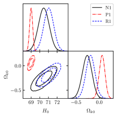
Lewisgetdist . The plots for the marginalized distributions with 1 and 2 confidence contours for and are shown in Figures
1, 2, 3 and 4 considering the squared exponential, Matérn , Cauchy and rational quadratic covariance
respectively.
The reconstructed for the N1 combination are consistent with spatial flatness within 2 confidence level (CL) for the squared exponential,
Matérn 9/2 and Cauchy covariance functions, and within 3 CL for the rational quadratic covariance. With the addition of BAO data in Set II, the
constraints on become tighter. From the combined N2 data-set, we find that is consistent with a spatially flat universe at 1 CL
for the squared exponential, Matérn 9/2 and Cauchy covariance, whereas in 2 for the rational quadratic kernel. The best-fit values shows an inclination
towards a closed universe for N1 and N2 data-sets. The degeneracy between and along with their correlation has also been shown.
We also examine if the two different strategies for determining value of , with conflicting results, affect the reconstruction significantly. We plot the
marginalized distributions with 1 and 2 confidence contours for and using the P1 and P2 combinations considering the P18
prior on , and for the R1 and R2 combinations considering the R19 prior on in figures 1-4. With the inclusion of the P18 data prior we see that the
best-fit values of favour a spatially open universe, whereas in case of the choice of R19 as a prior, the best-fit values of the constrained
shows that the combined data favours a spatially closed universe. However, a spatially flat universe is mostly included at 2 CL for both
cases.
| Dataset | ||||
|---|---|---|---|---|
| N1 | ||||
| N2 | ||||
| P1 | Sq. | |||
| P2 | Exp. | |||
| R1 | ||||
| R2 | ||||
| N1 | ||||
| N2 | ||||
| P1 | Mat. | |||
| P2 | 9/2 | |||
| R1 | ||||
| R2 | ||||
| N1 | ||||
| N2 | ||||
| P1 | ||||
| P2 | Cauchy | |||
| R1 | ||||
| R2 | ||||
| N1 | ||||
| N2 | ||||
| P1 | Rat. | |||
| P2 | Quad. | |||
| R1 | ||||
| R2 |
VI Thermodynamic consistency of constraints
In this section, the consistency of constraints obtained on with the second law of thermodynamics is looked at. We assume the universe as a system is bounded by a cosmological horizon, and the matter content of the universe is enclosed within a volume defined by a radius not bigger than the horizon gibbons ; jacob ; padma . In cosmology, the apparent horizon serves as the cosmological horizon, which is given by the equation , where is the proper radius of the 2-sphere and is the comoving radius. For the FLRW universe with a spatial curvature index , the apparent horizon is thus given by
| (24) |
For , the apparent horizon reduces to the Hubble horizon .
Now, the entropy of the horizon can be written as bak ,
| (25) |
For the second law to be valid, the entropy should be non-decreasing with respect to the expansion of the universe. If and stand for the entropy of the fluid describing the observable universe, and that of the horizon containing the fluid, respectively, then the total entropy of the system, i.e., , should satisfy the relation
| (26) |
Recently Ferreira and Pavónpavon gave a prescription to ascertain the signature of from the second law of thermodynamics. It is a fair assumption that the entropy of the observable universe is dominated by that of the cosmic horizon f_p_21 . So, the second law can be safely written as pavon ,
| (27) |
| (28) |
The inequality (28) can be rewritten, with a bit of simple algebraic exercise, as
| (29) |
Here is the deceleration parameter which gives a dimensionless measure of the cosmic acceleration and is defined as,
| (30) |
Testing the thermodynamic validity for the obtained constraints on requires a reconstruction of from the respective combination of data sets. Quite a lot of work on a non-parametric reconstruction of the cosmic deceleration parameter is already there in the literature. Some of them can be found in lin_q ; xia_q ; purba_q ; jesus_q ; purba_j ; keeley2020 . The list, however, is far from being exhaustive. We use the same datasets, that were used for the reconstruction of , to find the corresponding values of . A very brief methodology is the following. For a more detailed technical description, we refer to purba_int ; purba_q . The comoving distance , and its derivatives and are reconstructed w.r.t for different combinations of data sets. The uncertainty in from the corresponding data set is taken into account. For the CC and BAO data, we convert the - data to - data set using Eq. (9) and (13). is then connected to and via Eq. (12) as,
| (31) |
Thus, we take into account the data points, the uncertainty associated while performing the GP reconstruction. We add two extra points to the data set, and to the data before proceeding with the reconstruction. We obtain the reconstructed values of , and at the present epoch, along with their error uncertainties. Now, can be rewritten as a function of and its derivatives as,
| (32) |
VII Reconstruction along with the Perturbation data
Redshift-space distortions are an effect in observational cosmology where the spatial distribution of galaxies appears distorted when their positions are
looked at as a function of their redshift, rather than as functions of their distances. This effect occurs due to the peculiar velocities of the galaxies
causing a Doppler shift in addition to the redshift caused by the cosmological expansion. The growth of large structure can not only probe the background
evolution of the universe, but also distinguish between GR and different modified gravity theories ref39 ; ref41 . Recently, non-parametric
constraints on the Hubble parameter and the matter density parameter were obtained using the data from cosmic chronometers, type-Ia
supernovae, baryon acoustic oscillations and redshift-space distortions, assuming a spatially flat universe ref_new2022 . In this section, we
propose a non-parametric method to use the growth rate data measured from RSDs to constrain the spatial curvature.
| Set | |||||
|---|---|---|---|---|---|
| N3 | |||||
| N4 | |||||
| P3 | Sq. | ||||
| P4 | Exp. | ||||
| R3 | |||||
| R4 | |||||
| N3 | |||||
| N4 | |||||
| P3 | Mat. | ||||
| P4 | |||||
| R3 | |||||
| R4 | |||||
| N3 | |||||
| N4 | |||||
| P3 | |||||
| P4 | Cauchy | ||||
| R3 | |||||
| R4 | |||||
| N3 | |||||
| N4 | |||||
| P3 | Rat. | ||||
| P4 | Quad. | ||||
| R3 | |||||
| R4 |
In a background universe filled with matter and dark energy, the evolution of matter density contrast is given by,
| (33) |
In the linearized approximation, obeys the following second order differential equation for its evolution,
| (34) |
where is the background matter density, represents its first-order perturbation, and the ‘dot’ denotes derivative with respect to cosmic time . Note that is the effective gravitational constant. For Einstein’s GR, reduces to the Newton’s gravitational constant . Considering the growth factor , Gong, Ishak and Wanggong2009 provided an approximate solution to equation (34) as,
| (35) |
Here, is the matter density parameter, is the curvature density parameter and . The growth index depends on the model. For the CDM model, , and is a solution to Eq. (34) where the terms are neglected ref35 . For dark energy models with slowly varying equation of state ref36 . For modified gravity models, different values have been predicted in literature, such as for Dvali-Gabadadze-Porrati (DGP) model ref42 ; ref43 . The RSD data measure the quantity , defined by,
| (36) | |||||
where is the linear theory root-mean-square mass fluctuation within a sphere of radius Mpc ref21 ; ref22 ; ref23 ; ref24 ; ref25 ,
being the dimensionless Hubble parameter at the present epoch.
| (37) |


We proceed with the integration of Eq. (37) numerically using the composite trapezoidal rule as in equation (14). The reconstructed
function from CC and CC+BAO data are considered. For the Pantheon data, we make use of equations (16) and (17).
Here we consider the following combination of data sets,
-
•
Set III
-
1.
N3 - CC+SN+RSD
-
2.
P3 - CC+SN+RSD+P18
-
3.
R3 - CC+SN+RSD+R19
-
1.
-
•
Set IV
-
1.
N4 - CC+BAO+SN+RSD
-
2.
P4 - CC+BAO+SN+RSD+P18
-
3.
R4 - CC+BAO+SN+RSD+R19
-
1.
We use the GP method to reconstruct the function from RSD data. Finally, we constrain the cosmological parameters ,
, and utilizing the minimization technique. The uncertainties associated are estimated via a Markov
Chain Monte Carlo analysis. The best fit results along with their respective 1, 2 and 3 uncertainties is given in Table
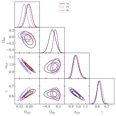
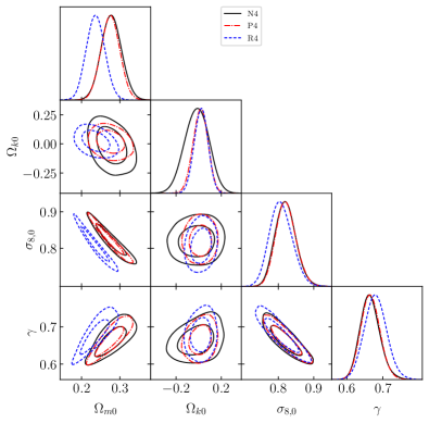
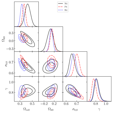
2. Plots for the marginalized posteriors with 1 and 2 confidence contours using the Set III and Set IV data
combinations are shown in Figures 5, 6, 7 and 8, for the squared exponential,
Matérn , Cauchy and rational quadratic covariance respectively.
The marginalized constraints for the N3 combination is consistent with spatial flatness within 1 CL for the squared exponential
and Matérn 9/2 covariance, within 2 for the Cauchy covariance and within 3 for the rational quadratic covariance. For the N4
combination, reconstructed lies with 1 for all four kernel choices. Considering the P18 and R19 prior, it is seen that
the squared exponential kernel includes for P3, P4, R4 combinations within 1 and for the R3 combination within 2. The
Matérn kernel includes for all P3, P4, R3, R4 combinations within 1. The Cauchy kernel includes for
the P3, R3 combination in 2, and for the P4, R4 combination in 1 CL. Lastly, utilizing the rational quadratic kernel,
is included in 3 for the P3 and R3 combination, whereas in 2 for the P4, R4 combination. Inclusion of BAO data leads to tighter
constraints on , and the best-fit values are seen to favour a spatially open universe (see Table 2).
The reconstructed values of show that the CDM model is mostly included in 2 and always in 3, except for the rational quadratic kernel. From Table 2, it can been seen that for the N4, P4 and R4 combinations, the CDM model in not included in 3 considering the rational quadratic kernel, and marginally included in 3 while using the Cauchy covariance.
VIII Discussion
In the present work, constraints on the cosmic curvature density parameter have been obtained from different cosmological probes with the
help of a non-parametric reconstruction. The Cosmic Chronometer and the radial Baryon Acoustic Oscillation measurements of the Hubble parameter, the
recent supernova compilation of the corrected Pantheon sample, along with measurement of the Redshift Space Distortions which measure the growth of large
structure are utilized for the purpose. The widely used Gaussian Process and the Markov Chain Monte Carlo method have been employed in this work. The
analysis has been performed for four choices of the covariance function, namely the squared exponential, Matérn , Cauchy and rational quadratic
kernel. The choice of covariance function involves some discretion and thus a bit subjective. The use of various choices of covariance makes the present
investigation quite exhaustive in that respect.
The reconstructed obtained by combining the CC and Pantheon data are consistent with spatial flatness within 1 confidence level for
the squared exponential covariance function, within 2 CL level for the Matérn 9/2 and Cauchy covariance function, and within 3 CL for
the rational quadratic covariance. Including the BAO data to the analysis results in tighter constraints on . Combining the CC and Pantheon
data with the BAO data, it can be seen that is consistent with a spatially flat universe at the 1 CL for the squared exponential,
Matérn 9/2 and Cauchy covariance, whereas in 2 for the rational quadratic kernel. The best-fit values show an inclination towards a closed
universe in these cases. This result is obtained without using any given priors. We then introduce the P18 and R19 measurements as priors in
our analysis and examine their effect on the reconstruction. Plots reveal that the best-fit values of favour a spatially open universe for
the P18 prior choice, whereas the R19 prior favours a spatially closed universe, except for the squared exponential kernel which favours a spatially open
universe for both the P18 and R19 priors. However, a spatially flat universe is mostly included at 2 CL for both cases (see Table 1).
Consistency with thermodynamic requirements imposed by the generalized second law of thermodynamics for the reconstructed constraints on
from the background data combinations are checked quite exhaustively. This has been done with the help of the inequality very recently given by Ferreira
and Pavónpavon (see also Ref. pavon2 ). It is quite encouraging to see that the constraints obtained are quite consistent with the
thermodynamic requirements, independent of the choice of the kernel for all possible combinations of data sets (see Table 1).
In addition to the background data, we also utilize the RSD data to determine using two combination of datasets, CC+Pantheon+RSD and
CC+BAO+Pantheon+RSD respectively. This inclusion does not help in providing tighter constraints on , but is essential as the spatial
curvature and the formation of large scale structure should be compatible. We also include the R18 and P18 priors and see their effect on the
reconstruction. The results obtained are consistent with spatial flatness mostly within 2 and always within 3 in the domain of the
reconstruction, (see Table 2).
The GP method has previously been used for constraining from observations. Li et al.li2016 constrained the spatial curvature
to be with 22 and Union 2.1 SN-Ia data, and considering the JLA
SN-Ia data, which are in good agreement with a spatially flat universe. Wei & Wuwei2017 extended this analysis using different priors and
showed that the local and global measurements can affect the constraints on . Wang et al.wang2017 showed that a spatially
flat and transparent universe is preferred by observations. The results indicated a strong degeneracy between the curvature parameter and cosmic opacity.
From 100 simulated GWs signals, Liaoliao2019 found the results favoured a spatially flat universe with uncertainty at 1, which was
reduced to for 1000 GWs signals. On combining with the SN-Ia data from DES, the uncertainty was further constrained to and respectively.
The analysis by Wei & Meliawei2019 suggests that a mildly closed universe () is preferred at the 1 level using
quasars and CC data. Recently, Wang, Ma & Xiawang2020 found a spatially open universe is favoured at 1 CL using 31 CC-H(z) measurements and
simulated data form GWs, based on the ANN method. Another non-parametric reconstruction of utilizing different approaches like the
principal component analysis, genetic algorithms, binning with direct error propagation and the Padé approximation, was carried out by Sapone, Majerotto
and Nesserisref_new2014 . Their results were in good agreement with at the 1 CL.
Our work is similar to the recent works by Yang & Gongyang2021 and Dhawan, Alsing & Vagonzzidhawan2021 , but there are quite a few differences
to list. Yang and Gongyang2021 , Dhawan, Alsing and Vagnozzidhawan2021 have used the Pantheon compilation by Scolnic et al.pan1
in their analysis. However, in this work we have utilized the very recent redshift corrected version of Pantheon compilation by Steinhardt, Sneppen and
Senpan_correct . Yang and Gongyang2021 reconstructed the quantity so that the discrepancy in the present value of Hubble
parameter is avoided. Dhawan, Alsing and Vagnozzidhawan2021 obtained constraints on independent of the absolute calibration of
either the SN-Ia or CC measurements. In this particular work, we have obtained constraints on both and form the combined CC+Pantheon
data, thereby capturing the degeneracy or correlation between them. Yang and Gongyang2021 imposed a zero mean function, which follows the work Seikel
et al.gp1 and is similar to our work. Dhawan, Alsing and Vagnozzidhawan2021 , on the other hand used a mean non-zero constant prior
equal to 100, following Shafieloo et al.gp2 . Utilizing solely the background data, Yang & Gongyang2021 found the case for a spatially
open universe from the combined CC and Pantheon data at more than 1 CL considering the squared exponential covariance. The present work starts with a
zero mean prior similar to yang2021 , but the best-fit value for the combined CC+Pantheon data (N1) using the same squared exponential kernel favours a
spatially closed universe, and is well included within in 1 CL. This result is similar in nature to that given by Dhawan, Alsing and
Vagnozzidhawan2021 where the obtained constraints on are consistent with spatial flatness at the
level. The qualitative difference of the present result with that obtained in yang2021 can stem from the fact that we have used the redshift corrected
version of the Pantheon compilationpan_correct .
Our conclusion is that although there is indeed a scope of revisiting the notion of a spatially flat universe, but the present state of affairs is still quite consistent with . Observations from future surveys, as well as more data on high redshift observations of CC, SN, BAO and other observables should be able to provide tighter constraints on .
References
- (1) A R Liddle, D H Lyth, Cosmological Inflation and Large Scale Structure; Cambridge University Press, Cambridge, UK (2000).
- (2) C. Clarkson, M. Cortes, and B. A. Bassett, J. Cosmol. Astropart. Phys. 08, 011 (2007).
- (3) Y.-G. Gong and A. Wang, Phys. Rev. D 75, 043520 (2007).
- (4) N. Aghanim et al. [Planck Collaboration], Astron. Astrophys. 641, A6 (2020).
- (5) C. D. Leonard, P. Bull, R. Allison, Phys. Rev. D 94, 023502 (2016).
- (6) A. Witzemann, P. Bull, C. Clarkson, M. G. Santos, M. Spinelli, A. Weltman, Mon. Not. R. Astron. Soc. 477, L122 (2018).
- (7) M. Denissenya, E. V. Linder, and A. Shafieloo J. Cosmol. Astropart. Phys. 03, 041 (2018).
- (8) S. Cao et al., Phys. Dark. Univ. 24, 100274 (2019).
- (9) E.-K. Li, M. Du and L. Xu, Mon. Not. R. Astron. Soc. 491, 4960 (2020).
- (10) G. Efstathiou and S. Gratton, Mon. Not. R. Astron. Soc. 496, L91 (2020).
- (11) C.-G. Park and B. Ratra, Phys. Rev. D 101, 083508 (2020)
- (12) R. C. Nunes and A. Bernui, Eur. Phys. J. C 80, 1025 (2020).
- (13) D. Benisty and D. Staicova, Astron. Astrophys. 647, A38 (2021)
- (14) W. Handley, Phys. Rev. D 103, 041301 (2021).
- (15) C. Clarkson, B. Bassett, and T. H.-C. Lu, Phys. Rev. Lett. 101, 011301 (2008).
- (16) R.-G. Cai, Z.-K. Guo, and T. Yang, Phys. Rev. D 93, 043517 (2016).
- (17) A. Rana, D. Jain, S. Mahajan, and A. Mukherjee, J. Cosmol. Astropart. Phys. 03, 028 (2017).
- (18) Y. Liu, S. Cao, T. Liu, X. Li, S. Geng, Y. Lian, and W. Guo, Astrophys. J. 901, 129 (2020).
- (19) R. Arjona, S. Nesseris, Phys. Rev. D 103, 103539 (2021).
- (20) D. Sapone, E. Majerotto, S. Nesseris, Phys. Rev. D 90, 023012 (2014).
- (21) Z. Li, G.-J. Wang, K. Liao, and Z.-H. Zhu, Astrophys. J. 833, 240 (2016).
- (22) J.-J. Wei and X.-F. Wu, Astrophys. J. 838, 160 (2017).
- (23) N. Suzuki, D. Rubin, C. Lidman et al., Astrophys. J. 746, 85 (2012).
- (24) M. Betoule et al. [SDSS Collaboration], Astron. Astrophys. 568, A22 (2014).
- (25) G.-J. Wang et al. Astrophys. J. 847 45 (2017).
- (26) K. Liao, Phys. Rev. D 99, 083514 (2019).
- (27) J.-J. Wei and F. Melia, Astrophys. J. 888, 99 (2020).
- (28) C.-Z. Ruan, F. Melia, Y. Chen, T.-J. Zhang, Astrophys. J. 881, 137 (2019).
- (29) H. Zhou and Z. Li, Astrophys. J. 889, 186 (2020).
- (30) B. Wang et al., Astrophys. J. 898, 100 (2020).
- (31) D. M. Scolnic et al., Astrophys. J. 859, 101 (2018).
- (32) G.-J. Wang, X.-J. Ma, J.-Q. Xia, Mon. Not. R. Astron. Soc. 501, 5714 (2021).
- (33) Y. Yang and Y. Gong, Mon. Not. R. Astron. Soc. 504, 3092 (2021).
- (34) S. Dhawan, J. Alsing, S. Vagnozzi, arXiv:2104.02485.
- (35) P. C. Ferreira and D. Pavón, Universe 2(4), 27 (2016).
- (36) C. Williams, Prediction with Gaussian Processes: From linear regression to linear prediction and beyond, Learning in Graphical Models, ed. Jordan M. I. (MIT Press, Cambridge, Massachusetts 1999).
- (37) D. MacKay, Information Theory, Inference and Learning Algorithms. (Cambridge Univ. Press, Cambridge, UK, 2003)
- (38) C. Rasmussen and C. Williams, Gaussian Processes for Machine Learning. (MIT Press, Cambridge, Massachusetts, 2006)
- (39) T. Holsclaw et al., Phys. Rev. Lett. 105, 241302 (2010).
- (40) M. Seikel, C. Clarkson and M. Smith, J. Cosmol. Astropart. Phys. 06, 036 (2012).
- (41) A. Shafieloo, A. G. Kim and E. V. Linder, Phys. Rev. D 85, 123530 (2012).
- (42) S. Yahya, M. Seikel, C. Clarkson, R. Maartens and M. Smith, Phys. Rev. D 89, 023503 (2014).
- (43) S. Santos-da Costa, V. C. Busti and R. F. Holanda, J. Cosmol. Astropart. Phys. 10, 061 (2015).
- (44) T. Yang, Z.-K. Guo and R.-G. Cai, Phys. Rev. D 91, 123533 (2015).
- (45) R.-G. Cai, Z.-K. Guo and T. Yang, Phys. Rev. D 93, 043517 (2016).
- (46) D. Wang and X.-H. Meng, Phys. Rev. D 95, 023508 (2017).
- (47) D. Wang, W. Zhang and X.-H. Meng, Eur. Phys. J. C 79, 211 (2019).
- (48) L. Zhou, X. Fu, Z. Peng and J. Chen, Phys. Rev. D 100, 123539 (2019).
- (49) Y.-F. Cai, M. Khurshudyan and E. N. Saridakis, Astrophys. J. 888, 62 (2020).
- (50) P. Mukherjee and N. Banerjee, arXiv:2007.15941
- (51) H.-N. Lin, X. Li and L. Tang, Chinese Phys. C. 43, 075101 (2019).
- (52) M.-J. Zhang, J.-Q. Xia, J. Cosmol. Astropart. Phys. 12, 005 (2016).
- (53) J. F. Jesus, R. Valentim, A. A. Escobal and S. H. Pereira, J. Cosmol. Astropart. Phys. 04, 053 (2020).
- (54) R. E. Keeley et al., arXiv:2010.03234.
- (55) P. Mukherjee and A. Mukherjee, Mon. Not. R. Astron. Soc. 504, 3938 (2021).
- (56) P. Mukherjee and N. Banerjee, Euro. Phys. J. C 81, 36 (2021).
- (57) P. Mukherjee and N. Banerjee, arXiv:2105.09995.
- (58) D. Benisty, Phys. Dark. Univ. 31, 100766 (2021).
- (59) K. Bora and S. Desai, arXiv:2104.00974.
- (60) R. Jimenez and A. Loeb, Astrophys. J. 573, 37 (2002).
- (61) J. Simon, L. Verde, and R. Jimenez, Phys. Rev. D 71, 123001 (2005).
- (62) C. Zhang, H. Zhang, S. Yuan, T.-J. Zhang and Y.-C. Sun, Res. Astron. Astrophys. 14, 1221 (2014).
- (63) D. Stern, R. Jimenez, L. Verde, M. Kamionkowski and S. A. Stanford, J. Cosmol. Astropart. Phys. 02, 008 (2010).
- (64) M. Moresco, A. Cimatti, R. Jimenez and L. Pozzetti, J. Cosmol. Astropart. Phys. 08, 006 (2012).
- (65) M. Moresco, Mon. Not. R. Astron. Soc. 450, L16 (2015).
- (66) M. Moresco, L. Pozzetti, A. Cimatti et al., J. Cosmol. Astropart. Phys. 05, 014 (2016).
- (67) A. L. Ratsimbazafy, S. I. Loubser, S. M. Crawford et al., Mon. Not. R. Astron. Soc. 467, 3239 (2017).
- (68) C. L. Steinhardt, A. Sneppen, and B. Sen, Astrophys. J. 902, 14 (2020).
- (69) E. Gaztanaga, A. Cabre, and L. Hui, Mon. Not. R. Astron. Soc. 399, 1663 (2009).
- (70) A. Oka, S. Saito, T. Nishimichi, A. Taruya, and K. Yamamoto, Mon. Not. R. Astron. Soc. 439, 2515 (2014).
- (71) Y. Wang et al. (BOSS), Mon. Not. R. Astron. Soc. 469, 3762 (2017).
- (72) C.-H. Chuang and Y. Wang, Mon. Not. R. Astron. Soc. 435, 255 (2013).
- (73) S. Alam et al. (BOSS), Mon. Not. R. Astron. Soc. 470, 2617 (2017).
- (74) C. Blake et al., Mon. Not. R. Astron. Soc. 425, 405 (2012).
- (75) C.-H. Chuang et al., Mon. Not. R. Astron. Soc., 433, 3559 (2013).
- (76) L. Anderson et al. (BOSS), Mon. Not. R. Astron. Soc. 441, 24 (2014).
- (77) G.-B. Zhao, et al., Mon. Not. R. Astron. Soc., 482, 3497 (2019).
- (78) N. G. Busca, T. Delubac, J. Rich et al., Astron. Astrophys., 552 A96 (2013).
- (79) J. E. Bautista et al., Astron. Astrophys. 603, A12 (2017).
- (80) T. Delubac et al. (BOSS), Astron. Astrophys. 574, A59 (2015).
- (81) A. Font-Ribera et al. (BOSS), J. Cosmol. Astropart. Phys. 05, 027 (2014).
- (82) E.-K. Li, M. Du, Z.-H. Zhou, H. Zhang and L. Xu, Mon. Not. R. Astron. Soc. 501, 4452 (2021).
- (83) A. G. Riess et al., Astrophys. J. 876, 85 (2019).
- (84) C. Blake et al., Mon. Not. R. Astron. Soc. 425, 405 (2012).
- (85) D. H. Jones et al., Mon. Not. R. Astron. Soc. 355, 747 (2004).
- (86) S. Alam et al. (SDSS-III), Astrophys. J. Suppl. 219, 12 (2015).
- (87) Y. Wang, G.-B. Zhao, C.-H. Chuang, M. Pellejero-Ibanez, C. Zhao, F.-S. Kitaura, and S. Rodriguez-Torres, Mon. Not. R. Astron. Soc. 481, 3160 (2018).
- (88) L. Guzzo et al., Astron. Astrophys. 566, A108 (2014).
- (89) A. de Mattia et al., arXiv:2007.09008.
- (90) A. Tamone et al., arXiv:2007.09009.
- (91) M. Aubert et al., arXiv:2007.09013.
- (92) G.-B. Zhao et al., arXiv:2007.09011.
- (93) H. Gil-Marín et al., arXiv:2007.08994.
- (94) R. Neveux et al., arXiv:2007.08999.
- (95) J. E. Bautista et al., arXiv:2007.08993.
- (96) K. Said, M. Colless, C. Magoulas, J. R. Lucey, and M. J. Hudson, Mon. Not. R. Astron. Soc. 497, 1275 (2020).
- (97) F. Qin, C. Howlett, and L. Staveley-Smith, Mon. Not. R. Astron. Soc. 487, 5235 (2019).
- (98) C. Blake, P. Carter, and J. Koda, Mon. Not. R. Astron. Soc. 479, 5168 (2018).
- (99) P. Zarrouk et al., Mon. Not. R. Astron. Soc. 477, 1639 (2018).
- (100) G.-B. Zhao et al., Mon. Not. R. Astron. Soc. 482, 3497 (2019).
- (101) R. Ruggeri et al., Mon. Not. R. Astron. Soc. 483, 3878 (2019).
- (102) C. Adams and C. Blake, Mon. Not. R. Astron. Soc. 471, 839 (2017).
- (103) Z. Li, Y. Jing, P. Zhang, and D. Cheng, Astrophys. J. 833, 287 (2016).
- (104) C.-H. Chuang et al. (BOSS), Mon. Not. R. Astron. Soc. 471, 2370 (2017).
- (105) A. G. Sanchez et al. (BOSS), Mon. Not. R. Astron. Soc. 464, 1640 (2017).
- (106) F. A. Marín, F. Beutler, C. Blake, J. Koda, E. Kazin, and D. P. Schneider, Mon. Not. R. Astron. Soc. 455, 4046 (2016).
- (107) Y. Wang, Mon. Not. R. Astron. Soc. 443, 2950 (2014).
- (108) S. Satpathy et al. (BOSS), Mon. Not. R. Astron. Soc. 469, 1369 (2017).
- (109) T. Okumura et al., Publ. Astron. Soc. Jap. 68, 38 (2016).
- (110) R. Holanda, J. Carvalho, and J. Alcaniz, J. Cosmol. Astropart. Phys. 04, 027 (2013).
- (111) R. Kessler and D. Scolnic, Astrophys. J. 836, 56 (2017).
- (112) D. Foreman-Mackey, D. W. Hogg, D. Lang and J. Goodman, Publ. Astron. Soc. Pac. 125, 306 (2013).
- (113) A. Lewis, arXiv:1910.13970.
- (114) G. W. Gibbons and S. W. Hawking, Phys. Rev. D 15, 2738 (1977).
- (115) T. Jacobson, Phys. Rev. Lett. 75, 1260 (1995).
- (116) T. Padmanabhan, Phys. Rept. 380, 235 (2003).
- (117) D. Bak and S. J. Rey, Class. Quant. Grav. 17, L83 (2000).
- (118) S. Frautschi, Science 217, 593 (1982).
- (119) D. Polarski, A. A. Starobinsky and H. Giacomini, J. Cosmol. Astropart. Phys. 12, 037 (2016).
- (120) L. Xu, Phys. Rev. D 88, 084032 (2013).
- (121) J. R.-Zapatero, C. García-García, D. Alonso, P. G. Ferreira and R. D. P. Grumitt, arXiv:2201.07025.
- (122) Y. Gong, M. Ishak, and A. Wang, Phys. Rev. D 80, 023002 (2009).
- (123) L.-M. Wang and P. J. Steinhardt, Astrophys. J. 508, 483 (1998).
- (124) E. V. Linder, Phys. Rev. D 72, 043529 (2005).
- (125) E. V. Linder and R. N. Cahn, Astropart. Phys. 28, 481 (2007).
- (126) H. Wei, Phys. Lett. B 664, 1 (2008).
- (127) Q. Gao and Y. Gong, Class. Quant. Grav. 31, 105007 (2014).
- (128) R. A. Battye, T. Charnock and A. Moss, Phys. Rev. D 91, 103508 (2015).
- (129) P. Bull et al., Phys. Dark Univ. 12, 56 (2016).
- (130) J. Sol Peracaula, J. d. C. Perez, and A. Gomez-Valent, Mon. Not. R. Astron. Soc. 478, 4357 (2018).
- (131) I. G. Mccarthy, S. Bird, J. Schaye, J. Harnois-Deraps, A. S. Font and L. Van Waerbeke, Mon. Not. R. Astron. Soc. 476, 2999 (2018).
- (132) J. P. Mimoso and D. Pavón, Phys. Rev. D, 94, 103507 (2016).