Constraining low redshift [C II] Emission by Cross-Correlating FIRAS and BOSS Data
Abstract
We perform a tomographic cross-correlation analysis of archival FIRAS data and the BOSS galaxy redshift survey to constrain the amplitude of [C II] fine structure emission. Our analysis employs spherical harmonic tomography (SHT), which is based on the angular cross-power spectrum between FIRAS maps and BOSS galaxy over-densities at each pair of redshift bins, over a redshift range of . We develop the SHT approach for intensity mapping, where it has several advantages over existing power spectral estimators. Our analysis constrains the product of the [C II] bias and [C II] specific intensity, , to be MJy/sr at and MJy/sr at at confidence. These limits are consistent with most current models of the [C II] signal, as well as with higher-redshift [C II] cross-power spectrum measurements from the Planck satellite and BOSS quasars. We also show that our analysis, if applied to data from a more sensitive instrument such as the proposed PIXIE satellite, can detect pessimistic [C II] models at high significance.
keywords:
galaxies: evolution – methods: data analysis – infrared: general1 Introduction
Atomic and molecular line emissions are powerful diagnostic tracers of the evolution of star formation over cosmic time. For instance, line emission studies may help reveal the causes of the significant decline in star formation rate after its peak at , inferred from observations of optical and infrared continuum radiation (Madau & Dickinson, 2014). One of the most useful lines for understanding the context of star formation is the [C II] fine structure line at GHz, which is the brightest cooling line in the far-infrared (FIR) spectrum, typically accounting for 0.1 to 1 of FIR energy (Stacey et al., 1991; Malhotra et al., 1997; Díaz-Santos et al., 2017). The bulk of this [C II] emission is expected to come from photodissociation regions (PDRs) on the edges of molecular gas clouds (Stacey et al., 2010). This association suggests that [C II] emission can trace the molecular gas available to fuel star formation. A study of galaxies detected by ALMA bore this out, finding that [C II] emission is linearly related to molecular gas content (Zanella et al., 2018). Measurements of [C II] emission and other lines (such as [C I] and the rotational transitions of CO) can be used in concert with galaxy formation models to constrain the physical properties of star-forming regions within galaxies (Popping et al., 2019; Yang et al., 2021).
Studies of line emission from individual galaxies (e.g., Carilli & Walter (2013); Hemmati et al. (2017); Zanella et al. (2018)) provide important insights into the [C II] luminosity function. However, they are subject to sample variance in small survey regions and are limited to galaxies above a brightness threshold, so they may not capture the cosmic average of the conditions of star formation. A complementary technique to individual galaxy studies is the technique of intensity mapping, which aims to map large-scale structure by detecting the aggregate redshifted line emission without cataloging individual sources (Hogan & Rees, 1979; Scott & Rees, 1990; Madau et al., 1997; Suginohara et al., 1999; Wyithe et al., 2008; Chang et al., 2008; Visbal et al., 2011; Kovetz et al., 2017, 2019). Some of the advantages of intensity mapping are that it captures all sources of emission rather than a biased sample of only the brightest sources. It also puts significantly lower requirements on telescope size, as the angular resolution need not be sufficient for individual source detection. Similarly, because individual objects do not need to be detected at a high signal-to-noise ratio, intensity mapping surveys can quickly cover large cosmic volumes, providing a complete census of emitting gas.
Intensity mapping has developed rapidly in the past fifteen years. Pathfinding intensity mapping surveys have used pre-existing telescopes to detect aggregate emission from the 21-cm line of neutral hydrogen (HI) (Pen et al., 2009; Chang et al., 2010; Masui et al., 2013; Switzer et al., 2013; Wolz et al., 2017; Anderson et al., 2018; Wolz et al., 2021) via cross-correlation with optical galaxy surveys. Several dedicated 21-cm intensity mapping experiments are now underway, targeting both the epoch of reionization (e.g., LOFAR, van Haarlem et al. (2013), and SKA precursors HERA and MWA, DeBoer et al. (2017); McKinley et al. (2018)) as well as the era of dark energy dominance (e.g., CHIME, Bandura et al. (2014), Tianlai, Chen (2012), HIRAX, Crichton et al. (2021), SKA precursor MeerKAT, Wang et al. (2021), and BINGO, Abdalla et al. (2021)). The initial focus on the 21-cm line has expanded to include [C II], the rotational lines of CO, Lyman , H, H, and more (Kovetz et al., 2019).
The COPPS survey has utilized the Sunyaev-Zel’dovich Array (SZA) to make tentative detections of CO emission at in cross-correlation with spectroscopic galaxy surveys (Keenan et al., 2021) and auto-correlation in the shot-noise regime (Keating et al., 2016). A similar CO shot-noise detection was made with Millimeter-wave Intensity Mapping Experiment (mmIME), using ALMA and ACA facilities (Keating et al., 2020). Among a new generation of dedicated ground-based intensity mapping instruments targeting CO and [C II] are COMAP (Cleary et al., 2021), designed to measure CO(1-0) from and CO(2-1) at , TIME (Crites et al., 2014), targeting [C II] emission from the epoch of reionization and CO from , CONCERTO (The CONCERTO collaboration et al., 2020), focusing on [C II] emission from the epoch of reionization, the CCAT-prime receiver for the FYST (CCAT-Prime collaboration et al., 2021), which targets [C II] at and [OIII] at , and SPT-SLIM (Karkare et al., 2022), which aims to use the South Pole Telescope to target several CO transitions from . Two NASA balloon experiments designed to measure line emission in the far-infrared (FIR) are TIM (Vieira et al., 2020), focusing on [C II] at , and EXCLAIM (Cataldo et al., 2021), focusing on CO and [C II] in windows from . The NASA MIDEX-class satellite mission, SPHEREx, will produce intensity maps of multiple lines, including H, H, [OII], and [OIII] at (Gong et al., 2017).
The brightness of the [C II] line makes it an excellent candidate for the technique of line intensity mapping. Pullen et al. (2018) recently demonstrated the promise of [C II] intensity mapping through an analysis of the cross-correlation between the angular distribution of high-redshift () quasars in the BOSS survey and the , , and GHz Planck maps. They found a cross-correlation exceeding the expected thermal continuum at GHz, consistent with [C II] emission correlated with BOSS quasars. A refinement of the analysis (Yang et al., 2019) increased the result’s significance. Still, the authors caution that greater spectral resolution is required to verify that the excess cross-correlation is explained by [C II] emission rather than the redshift evolution of the correlated continuum emission.
Switzer (2017a) describes how future instruments for measuring spectral distortions in the cosmic microwave background (CMB) can be employed for intensity mapping. To anticipate the capabilities of future measurements, we use data from the COBE-FIRAS instrument (Fixsen et al., 1994), in cross-correlation with the BOSS CMASS and LOWZ galaxy catalogs, to make the first tomographic intensity mapping constraint on [C II] emission. The FIRAS instrument (Fixsen et al., 1994) was designed to precisely measure the spectrum of the CMB, dust, and line emission from the Milky Way. It covers a broad frequency range from GHz to GHz with GHz spectral channels. This, and the fact that FIRAS’ frequency range conveniently overlaps the well-sampled LOWZ and CMASS galaxy catalogs, make FIRASBOSS a natural candidate for a tomographic [C II] cross-correlation analysis.
Compared to the Planck data set used by Pullen et al. (2018), the FIRAS data set has much higher thermal noise per pixel and much lower angular resolution (the FIRAS beam has nearly a 7-degree full-width-half-maximum). At first glance, it seems that these limitations give FIRASBOSS no hope of approaching the sensitivity of PlanckQSO, but we achieve error bars that are only about two times larger. One reason is that the effective number of independent modes scales with the number of redshift bins. We use 14 redshift bins for FIRASCMASS and 16 for FIRASLOWZ, whereas PlanckQSO only has one channel with correlated [C II] signal. However, the number of modes also depends on the range of measurable angular scales, and PlanckQSO more than makes up for its lack of redshift resolution with its much larger range of observable angular modes. Counteracting this, FIRASBOSS sees a larger cosmological signal due to structure growth at lower redshifts, and, critically, the CMASS and LOWZ galaxy catalogs are well-sampled enough that shot noise is subdominant at the redshifts and angular scales we consider. The BOSS quasar sample used in PlanckQSO, on the other hand, is dominated by shot noise due to the sparser sampling.
1.1 Spherical harmonic tomography
We cross-correlate FIRAS data with cosmological overdensity inferred from the BOSS spectroscopic galaxy redshift survey to search for extragalactic [C II] emission. Two competing effects make the BOSS CMASS () and LOWZ () especially well-tuned for this goal. The growth of large-scale structure and geometric factors yield increasing density contrast on large angular scales where FIRAS is most sensitive. However, by ( GHz), the FIRAS noise rises dramatically. For our analysis, we bin the CMASS and LOWZ galaxy maps into redshift slices that correspond to the FIRAS frequency channels for the [C II] line. We then use the technique of spherical harmonic tomography (SHT) (see, for example, Asorey et al. (2012); Nicola et al. (2014); Lanusse et al. (2015)) to compute the angular cross-power spectrum, , between the FIRAS maps and BOSS galaxy over-densities at each pair of redshifts.
With a fine enough binning in redshift, SHT captures the complete information available in the power spectrum (Asorey et al., 2012), and it is well-matched to large area surveys such as BOSS, where a flat-sky approximation would introduce significant distortions. In order to fit our data to a model, the expected angular clustering signal, , must be computed by integrating a 3D power spectrum model over highly oscillatory Bessel functions (details included in Section 4.1). Standard anisotropy codes, such as CAMB (Lewis & Challinor, 2011) and CLASS (Di Dio et al., 2013, 2014), include methods for performing this integration (with or without the Limber approximation).
We describe the analysis over several sections. Section 2 motivates the statistic, explains how to use the pseudo- technique to compute for surveys with partial sky coverage, and describes the likelihood function we use for parameter estimation with . Section 3 describes the FIRAS dataset, viewed as a [C II] intensity map, and the BOSS CMASS and LOWZ data sets, viewed as binned galaxy over-density maps. Section 4 describes our dark matter model and its use in fitting the [C II] and CIB amplitude to our FIRASBOSS data. It also describes how we model the FIRASBOSS covariance by fitting parametric models to the BOSSBOSS and FIRASFIRAS data. Section 5 discusses our [C II] constraints and how they relate to other measurements and astrophysical models. We conclude in Section 6.
2 Parameter Estimation with the Statistic
2.1 Motivating the estimator
We perform our analysis with Spherical Harmonic Tomography (SHT), a two-point statistic wherein each redshift slice of data is decomposed into spherical harmonics, and the angular power spectrum, , is calculated between each pair of redshift slices. SHT captures the complete information available in the more typically used three-dimensional power spectrum statistic, (Asorey et al., 2012). The SHT technique has already been used in several clustering analyses and forecasts for galaxy surveys (e.g. Thomas et al. (2011); Leistedt et al. (2013); Balaguera-Antolínez et al. (2018); Loureiro et al. (2019a); Xavier et al. (2019); Fonseca et al. (2019); Nicola et al. (2020); Viljoen et al. (2020); Tanidis & Camera (2021)). Among these, a recent analysis of BOSS CMASS and LOWZ clustering using Spherical Harmonic Tomography (Loureiro et al., 2019a) found equivalent or better constraints on cosmological parameters compared to standard power spectrum analysis techniques. As the set of two-point cross-correlations, the SHT contains all information in the data cubes that is statistically isotropic and Gaussian.
SHT has some inherent geometrical advantages, especially for large-angle and deep surveys. A significant advantage is that the spherical coordinates apply to wide-angle surveys like BOSS without any flat-sky approximation. A traditional analysis relies on the flat-sky approximation to distinguish between transverse and line-of-sight modes, which is critical for accurately representing redshift space distortions (RSDs) and distinguishing continuum foregrounds from line signal. By contrast, in the SHT formalism, both foregrounds and linear redshift space distortions take exact, simple forms. This geometric advantage is shared with the related analysis technique of spherical Fourier-Bessel (SFB) decomposition (Fisher et al., 1995; Heavens & Taylor, 1995; Rassat & Refregier, 2012; Leistedt et al., 2012; Yoo & Desjacques, 2013; Lanusse et al., 2015; Liu et al., 2016; Grasshorn Gebhardt & Doré, 2021), which, in addtion to spherical harmonic decomposition, involves a further Fourier-Bessel transform and data-compression along the line-of-sight. However, SFB does not share another important feature of SHT, which is its ability to capture redshift-dependent change over cosmological time in deep surveys. For deep surveys, structure growth and changes in star formation rate break the assumption of translational invariance in the line-of-sight direction, rendering the or SFB statistic insufficient. However, since does not compress data along the line-of-sight direction, it describes redshift evolution. A study (Mondal et al., 2022) of simulated 21-cm data from the Epoch of Reionization (EoR) found that an implementation of the SHT technique, MAPS (Mondal et al., 2018; Mondal et al., 2019; Mondal et al., 2020), obtains 2 times more stringent error bars on model parameters than techniques that fail to capture redshift evolution due to data compression along the line-of-sight, such as or SFB. A final geometric advantage is that describes the data in observing coordinates of angle and frequency (or, equivalently, redshift) rather than re-gridding the data onto cosmological distances in an assumed cosmological model. An MCMC likelihood analysis that constrains cosmological parameters would therefore not need to recompute the data statistic at each step, which in principle would be needed for a or SFB analysis.
There are several practical advantages to parameter estimation with SHT. Due to the scan strategy, intensity mapping data generally have inhomogeneous noise and partial sky coverage in the angular direction. Multiplication by noise weights in real space couples transverse modes in Fourier space, which can be easily accounted for in SHT analysis, thanks to pre-existing work (Hivon et al., 2002; Tristram et al., 2005) on the pseudo- technique from CMB analysis. Intensity maps will also often have significant variation in the noise level in the frequency (line-of-sight) direction because of variations in spectrometer noise or chromatic contamination such as terrestrial radio frequency interference. Inhomogeneous noise in real space produces coupling of line-of-sight Fourier modes in analyses of . In contrast, because does not perform any Fourier or Bessel transform in the redshift direction, no coupling occurs, and the noise can be expressed as a simple function of the redshift slice. Additionally, chromatic beam effects can be modeled per redshift slice without introducing any flat-sky approximation.
In addition, SHT provides an avenue for self-consistently handling foregrounds and other continuum signals. In contrast, other approaches that remove foregrounds in map space before the two-point analysis must contend with signal loss (Switzer et al., 2015; Cheng et al., 2018). With SHT, the covariance of can be constructed to include information about foregrounds. The inverse covariance weights the data in the likelihood analysis for the line brightness, suppressing modes contaminated by foregrounds self-consistently with the parameter estimation. Additionally, the model can include signal terms such as the cross-correlation of a galaxy redshift sample with the correlated continuum emission of the galaxies in the IM volume (Serra et al., 2014a; Pullen et al., 2018; Switzer et al., 2019).
SHT also introduces several new challenges to the analysis. First, it places significant requirements on memory for the computation of the likelihood. This is because the size of the covariance scales as , where is the number of redshift bins and is the number of angular bins. For FIRAS, this is fairly manageable because we analyze only three angular bins and about 15 redshift slices for each of FIRASCMASS and FIRASLOWZ. The size of the covariance will be more challenging for future instruments with higher spectral and angular resolution.
The visualization of and its errors presents an additional challenge. The extra dimensionality of , which allows it to measure redshift evolution, also means that angular and redshift information cannot be shown in a single plot. We develop several approaches for displaying the data and describing the goodness of fit to high-dimensional data with complex covariance. Lastly, the evaluation of the model is computationally expensive. Since the current generation of IM observations focuses on detection and measurements of line brightness (Kovetz et al., 2019), this is not an issue. In this regime, the model can be constructed from linear combinations of cosmological clustering and shot noise templates that need only be calculated once. In contrast, studies of large-scale structure acquire information from the nonlinear dependence of on cosmological parameters, so can require expensive recalculation of the anisotropy. Recent work has accelerated the integrals that convert to without using the Limber approximation (Campagne et al., 2017; Schöneberg et al., 2018), making cosmological parameter estimation with more practical.
2.2 Computing with Incomplete Sky Coverage
Extensive work in CMB data analysis has developed an approach (Hivon et al., 2002) for dealing with incomplete sky coverage and an approximate formula for the covariance it induces between angular scales (Tristram et al., 2005). The code package NaMaster (Alonso et al., 2019; Alonso, 2018) includes this full functionality, along with contaminant removal for polarized and unpolarized maps, on both large curved-sky maps and small maps, using a flat-sky approximation.
For observed maps A and B with known, possibly different, inverse noise weights and beams, the angular power spectrum of the inverse noise weighted maps is the pseudo- spectrum (Hivon et al., 2002), which we label , following the notation of Tristram et al. (2005). The pseudo- spectrum is related to the true full-sky angular power spectrum by
| (1) |
where is the product of the beam and pixel window function of map A, is the product of the beam and pixel window function of map B, and is the mixing matrix, computed via
| (2) |
where is the angular power spectrum of the inverse noise spatial weights of maps and , and represents a Wigner 3-j symbol. These formulas work for both auto and cross-correlations. The mixing matrix is not invertible with partial sky coverage, and it is convenient to define the binned pseudo- spectrum and binned mixing matrix. Here, a range of multipoles are combined into a bandpower , for which the mixing matrix of bandpowers and is invertible using suitable binning. Define as a binning matrix that averages blocks of consecutive s into bins indexed by and define as an equivalent unbinning matrix that assigns the average value of a bin to each within that bin. Then, define the binned quantities
| (3) |
If the bin size is wide enough, is invertible even for partial sky coverage. One can then form an estimate, , of the binned angular power spectrum from the observed binned pseudo- spectrum, , via
| (4) |
This procedure should only recover the true angular power spectrum if is constant within each bin . Since this is not generally the case, to compare to a model , as we do in Section 4, we always compute or simulate the expected binned angular power spectrum, , which is related to the model via
| (5) |
If one assumes that the true distribution is Gaussian, then the terms of the covariance can be roughly approximated as
| (6) |
where is the fraction of the sky seen by the survey and is the width of the bin centered at . For intensity mapping tomography, the first term is the product of the autopower of the IM data and the galaxy survey , and the second term is the product of cross-powers between the IM data and the galaxy survey. For the FIRASBOSS analysis, the first term dominates the covariance due to the high thermal noise and large (at low ) Milky Way foreground signal present in . So, as a rough rule of thumb, the terms of the cross-power covariance are
| (7) |
Appendix A applies this equation to derive an approximate formula for the expected sensitivity that a cross-power survey could achieve on the line intensity. The covariance can be more accurately approximated under the assumption of large sky coverage (Tristram et al. (2005), formula included in Appendix C) or computed via simulated draws from an assumed model and repeated pseudo- computation of the resulting . For our BOSSBOSS analysis, we use the approximate covariance of Tristram et al. (2005), as it matches our simulations well. For the FIRASFIRAS and FIRASBOSS analysis, the approximation fails to match simulations, so we instead use a fully simulated covariance. We suspect that the inconsistency between the simulations and the approximate formula is due to the combination of small sky coverage and the steep angular index of the Milky Way foregrounds. Further details on the covariance used for each analysis are included in Section 4.3.
2.3 Implementing the estimator
For a range of binned multipoles indexed by bandpower , the computed is a rank-3 tensor, indexed by , , and . To perform a likelihood analysis, we define as a flattened vector of all the unique elements of .
| (8) |
Note that for auto-powers, there are only unique elements, since . For the cross-power, all elements are unique, and has a length of .
The likelihood formed from is well-studied in CMB literature (see e.g., Hamimeche & Lewis (2008) for a survey of likelihood forms depending on assumptions). If the amplitudes of the spherical harmonics of the maps are drawn from an underlying Gaussian distribution, then the resulting measured vector of anisotropies, , is Wishart-distributed. With our bin size of , and for the -range with signal sensitivity (see Figure 7), the number of modes contributing to each bin is high enough that the Wishart distribution is reasonably well-approximated by a Gaussian distribution
| (9) |
where is the bandpower covariance matrix of the flattened data vector and includes binned angular coupling induced by incomplete sky coverage, is a flattened vector of the estimate computed from the data, and is a flattened vector of the model, which depends on the science parameters of interest, .
When analyzing multiple datasets, such as galaxy surveys and intensity maps, the likelihood can be expanded to apply to a data vector that concatenates the auto- and cross-powers of all the datasets. So, for the FIRAS and BOSS data, the data vector could contain flattened FIRASFIRAS, BOSSBOSS, and FIRASBOSS estimates. If the thermal noise and galaxy shot noise were small, then the high correlation between the galaxy data and [C II] data, which trace the same matter fluctuations, could be exploited to remove cosmic variance from the measurement of the [C II] line intensity (McDonald & Seljak, 2009; Bull et al., 2015; Abramo et al., 2016; Switzer, 2017b; Switzer et al., 2019; Oxholm & Switzer, 2021). For this FIRASBOSS analysis, thermal noise and foregrounds, rather than cosmic variance, are dominant sources of error, so the benefits of such an approach are negligible. However, future intensity mapping experiments may benefit from this approach. For simplicity, we focus on [C II] constraints from the cross-power, FIRASBOSS, and we only use FIRASFIRAS and BOSSBOSS to validate the cross-power covariance model.
3 The FIRAS and BOSS data sets
3.1 FIRAS Instrument and Data Set

FIRAS is a rapid-scan polarizing Michelson interferometer (Mather et al., 1993) on the COBE satellite that mapped the frequency spectrum of the full infrared sky at a coarse angular resolution. The frequency spectrum for each pointing was obtained via an inverse Fourier transform of the interferogram of measured powers over a discrete range of instrument path length differences. The resulting measurements of the sky spectrum are equal to the true spectrum convolved by the inverse Fourier transform of an apodization function (Fixsen et al., 1994). Figure 1 plots this frequency response function, which we shall denote .
The published FIRAS maps are binned in the HEALPix 111http://healpix.sourceforge.net (Górski et al., 2005; Zonca et al., 2019) format with resolution parameter , corresponding to 3072 angular pixels, sufficient to sample the 7-degree beam. In addition to the sky maps, inverse-noise weight maps were produced based on fluctuations of the different interferograms contributing to each pixel. We upgrade the map binning to for analysis. This regridding does not gain any angular information from the FIRAS maps, but it allows finer, more accurate noise weights for the galaxy over-density maps. Figure 2 shows the inverse-noise weights at for [C II] emission from .

The FIRAS beam is formed by a non-imaging parabolic concentrator, which creates a near-tophat beam response with 7-degree FWHM. This beam was measured by in-flight scans of the Moon (Figure 3). In addition to this intrinsic beam convolution, the finite time required to complete an interferogram combined with the FIRAS scan motion causes the maps to be further smoothed in the ecliptic scan direction by a 2.4-degree tophat function. We account for all beam, scan, and pixelization smoothing effects on the power spectrum via simulation: realizations of a model power spectrum are drawn at , convolved by the FIRAS beam model, convolved by a 2.4-degree tophat function in the ecliptic direction, degraded to , and re-grid onto . We then compute an angular transfer function in by calculating the ratio of the angular power spectrum calculated from these modified maps to the original angular power spectrum. The square root of this transfer function, denoted (Figure 4), represents the combined beam, scan, and pixel window function for the FIRAS maps.


3.2 BOSS Data Set
The BOSS survey (Dawson et al., 2012) extends the Sloan Digital Sky Survey (SDSS). It was designed to measure the Baryon Acoustic Oscillation feature in the galaxy matter power spectrum. Precise spectroscopic redshifts were obtained for approximately 1.5 million galaxies in the redshift range , selected to have approximately constant stellar mass. Details about the telescope and instruments of SDSS can be found in Fukugita et al. (1996), Gunn et al. (1998), Gunn et al. (2006), Doi et al. (2010), and Smee et al. (2013).

BOSS data release 12 (Alam et al., 2015) includes 100 mock unclustered realizations of CMASS and LOWZ galaxies. We bin both the real catalogs and the unclustered mocks onto HealPix maps with , in redshift bins corresponding precisely to the FIRAS frequency bins under the assumption that the FIRAS signal is redshifted [C II] emission. We construct the CMASS and LOWZ galaxy selection functions, denoted , by averaging their mock catalogs, assuming a selection function that is separable in angle and redshift. The separability assumption reduces shot noise in the selection function and should be sufficiently accurate for the cross-correlation, limited by FIRAS noise. We define the boundary of the survey by zeroing pixel weights where the selection function is more than standard deviations below the angular average of the sample, which additionally de-weights some regions with lower coverage. The galaxy over-density field is then formed via
| (10) |
where denotes the binned galaxy maps and denotes the selection function. Figure 6 displays the galaxy over-density maps and selection function for a single redshift slice at .

Previous analysis of the BOSS data has found evidence of systematic contamination from stellar populations at low (Loureiro et al., 2019a). We also find evidence of systematic low contamination, with spurious correlations visible at the lowest -bin of our analysis (), indicative of a common systematic component across redshifts. tests of BOSS data compared to our fitted model are high when including this bin. However, they drop to expected values when excluding this bin. We cut this lowest angular bin and the next bin () from our analysis (see Figure 7).
4 Signal Model and Parameter Fit
The low spatial resolution of the FIRAS maps limits the range of scales to , or five bandpowers with . Figure 7 shows the expected variance on the cross-power signal for each and the -bins we use in this analysis. Since the first of the five available -bins shows signs of stellar contamination in the BOSS sample, we drop it from our analysis. We also eliminate the second -bin because, in that bin, the mode mixing caused by partial sky coverage combines with the steep angular index of Milky Way emission to mix the FIRAS auto-power negative. This makes the empirical FIRAS model non-positive definite in that bin and therefore unusable as verification for our cross-power fits. Consequently, we use only the last three bins, as indicated in Figure 7, which contain most of the sensitivity. In principle, extra information could be obtained at higher by re-making the FIRAS maps from the raw data at higher , but in practice, the 7-degree beam of the FIRAS instrument diminishes the signal-to-noise ratio at higher s (see the upward trend in noise-to-signal ratio for at in Figure 7). To model the errors, we also restrict the FIRASFIRAS and BOSSBOSS analysis to these same 3 -bins, even though much higher information is available from the BOSS catalog. Similarly, we must restrict the FIRASFIRAS analysis to the sky fraction covered by the BOSS galaxy survey to avoid over-estimating the error bars by including the bright Galactic plane, which has no overlap with the BOSS North or South fields.

4.1 Dark Matter Model
Both our BOSSBOSS and FIRASBOSS models require the dark matter angular power spectrum of the overdensity field, . We calculate this angular power spectrum with the Boltzmann code CLASS (Di Dio et al., 2013, 2014), using cosmological parameters inferred from the Planck 2015 (Ade et al., 2016) temperature and low- polarization maps (TT+LowP). The Halofit routine (Smith et al., 2003) provides nonlinear corrections to the power spectrum. However, on the several-degree scales of this analysis, the fluctuations are well-described by linear perturbation theory ( h/Mpc h/Mpc), and nonlinear corrections are small. CLASS computes the angular power spectrum from the 3D power spectrum, , according to the equation
| (11) |
where is the dark matter power spectrum at the current epoch, and, if there are no redshift space distortions (RSDs),
| (12) |
where is the bias for dark matter tracer , is a tophat redshift selection function that is non-zero only over the range of the redshift slice centered at redshift and normalized to integrate to 1, is a spherical Bessel function of the first kind with parameter , is the growth factor, and is the radial comoving distance to the shell at redshift . Linear redshift space distortions (RSDs) can be included (Fisher et al., 1994; Padmanabhan et al., 2007) by replacing with , where
| (13) |
where , with being the logarithmic growth rate of linear perturbations in the matter power spectrum. The that results from using and contains cosmological terms proportional to , proportional to , and independent of both and . We label these terms , , and respectively. They are calculated from CLASS via linear combinations of computations without RSD and bias 1, with RSD and bias 1, and with RSD and bias 0. With this formalism, the cross-power spectrum of two biased matter tracers is given by
| (14) |
The bias dependence of these terms is reminiscent of the Kaiser correction in power spectrum space. Indeed, these equations can be derived by including the Kaiser enhancement term in a plane-wave expansion of the power spectrum and integrating along the line-of-sight (Padmanabhan et al., 2007).
We do not model finger-of-God effects or redshift smearing due to spectroscopic survey errors since our redshift bin size of is more than 10 times larger than the 400 km/s satellite galaxy velocity dispersion fit and 30 km/s spectroscopic error fit found by Guo et al. (2015)’s analysis of CMASS galaxies. Analyses with sufficient redshift resolution to resolve the finger-of-God effect can include it in the signal model by smoothing the radial window function in the calculation (Loureiro et al., 2019b; Grasshorn Gebhardt & Jeong, 2020).
4.2 FIRASBOSS
The cross-correlation signal model consists solely of correlated continuum emission (dust) and [C II] emission from the BOSS galaxies. Because they are uncorrelated with the cosmological overdensity field, the thermal noise and foregrounds contribute zero average cross-power and thus will not factor into the mean signal model (although the variance caused by their spurious correlation with the galaxy survey will be included through the FIRAS auto-power in the covariance).
In Appendix B, we derive the functional form of our cross-power model. The [C II] part of the model is
| (15) |
The redshift dependence of is shown in Equation 36. An intensity mapping experiment with sufficient sensitivity can fit the parameters that control the redshift evolution of . However, due to the high noise and large beam of FIRAS, we fix all of those evolution parameters with reasonable values from Pullen et al. (2018) (see details in Appendix B). Those values lead to a modest evolution in which the brightness increases toward higher redshift over each of the CMASS and LOWZ redshift ranges. Our MCMC analysis assumes this redshift shape and fits for the overall amplitude of at the central redshift of each region (CMASS and LOWZ, respectively).
The CIB portion of the cross-power model is
| (16) |
where is the intensity of the CIB that is emitted from sources in a redshift bin of size , centered at redshift , and measured at a frequency of . The sum over in Equation 16 should, in principle, be carried out over all redshifts, even those outside of the galaxy survey. In practice, for the redshift bins and bins considered in this analysis, the bracketed kernel is dominated by the term, with the neighboring off-diagonal terms around 20% of the diagonal term, and the rest of the terms are negligible. As with our [C II] analysis, because of the limited sensitivity of the FIRAS data, we do not attempt to constrain the redshift evolution of the CIB brightness or the spectral shape of the CIB emission. Instead, these are fixed by the assumed values of (Planck Collaboration et al., 2014b), K (Serra et al., 2014a), (Pullen et al., 2018), (Planck Collaboration et al., 2014b; Serra et al., 2016), and (Shang et al., 2012; Planck Collaboration et al., 2014b; Serra et al., 2016). Because of this assumed spectral and redshift evolution, the parameter we constrain is , where is the central redshift of the analysis region, and is the corresponding central frequency of the analysis region.
Finally, our signal model must account for the FIRAS data being convolved by the FIRAS frequency response function, . To do this, we convert the frequency response function to a function of redshift, , and convolve by , resulting in the final signal model
| (17) |
In our MCMC analysis, we fix the value of the galaxy bias, , to the best-fit value from our BOSSBOSS analysis (Section 4.3.2) and also fix the [C II] and CIB bias to be identical to the galaxy bias (). This fixing of the [C II]/CIB bias has almost no effect on our fits since only the small RSD terms ( and ) can break the degeneracy between and , and FIRASBOSS lacks the precision to break that degeneracy. The next section, 4.3 develops the covariance model employed by the MCMC.
Figure 8 shows the MCMC contours for our parameter fits to the FIRASBOSS data with the CMASS and LOWZ galaxies. Also shown, on the bottom row, are the of the CMASS and LOWZ maximum likelihood fits, compared to a simulated distribution of best-fit values. For the MCMC analysis, we apply a simple flat prior that restricts both and to positive values. This prior has almost no effect on our best-fit values, but since we do not have enough sensitivity for detection, it prevents unphysical negative values from counting towards our quoted upper limit constraints. We find, at 95 percent confidence, that MJy/sr at and MJy/sr at .

4.3 Modeling the FIRASBOSS Covariance
The required pieces for the covariance used in the MCMC parameter estimation are models for: 1) the [C II] and CIB signal associated with cosmological clustering, 2) the BOSS signal associated with cosmological clustering, plus shot noise, and 3) the FIRAS thermal noise and foregrounds. In the following three subsections, we describe each of these models in turn. Appendix D describes our method of simulating the covariance from these three models.
4.3.1 [C II] and CIB signal
We simulate the [C II] and CIB variance models through map-space simulations that include FIRAS instrumental effects. The [C II] and CIB signals are painted onto maps drawn from the cosmological clustering signal with linear bias. For the [C II] signal, this is accomplished by multiplying the drawn maps by . For the CIB signal, the maps are matrix-multiplied by , in a map-space analogy to Equation 16. These maps are then convolved by the FIRAS redshift response function, .
The magnitude of the portion of the covariance that comes from this [C II] and CIB signal is a function of the [C II] and CIB amplitudes. In order to account for this, our covariance is constructed from a linear combination of four separate simulations (accounting for each cross-term). Appendix D describes this process.
4.3.2 Clustering signal and shot noise from BOSSBOSS
We model the variance in the BOSS survey as a tracer of the dark matter with constant bias and linear RSD plus shot noise, or
| (18) |
where is the average number of BOSS galaxies per pixel in each redshift slice, and is the angular size of a pixel in steradians. While the complete BOSSBOSS power spectrum requires additional modeling to describe all scales (Loureiro et al., 2019a), this simple model with free parameters for a constant bias and shot-noise amplitude is sufficient to describe the BOSS variance relevant to the angular scales analyzed in FIRASBOSS. Due to the large number of galaxies in the CMASS and LOWZ samples and the limited -range of our analysis, the shot noise is considerably smaller than the clustering signal, so is weakly constrained. The bias parameter is fit to a value of 1.81 and 1.82 for the LOWZ and CMASS samples, consistent with previous work (Salazar-Albornoz et al., 2017). We find reasonable values for both the CMASS ( per degree of freedom of 1.02, PTE of 0.37) and LOWZ ( per degree of freedom of 1.08, PTE of 0.12) fits. Figure 9 shows the measured from CMASS versus the best-fit model for the three -bins we consider.
The covariance we use for the BOSSBOSS parameter estimation is computed using the approximate formula of Tristram et al. (2005) described in Appendix C. Since the covariance is a function of the model, an MCMC analysis must, in principle, recalculate the covariance for each different estimate of the underlying model parameters. For BOSSBOSS, we instead employ an iterative approach. We make a best guess of the parameters, compute a covariance for that guess, find a new maximum likelihood solution using that covariance, and then repeat the procedure. After several iterations, this procedure has converged, and the parameters assumed in the model for the covariance equal the parameters at the maximum likelihood peak of our MCMC fit to within a fractional tolerance of .

4.3.3 Thermal noise and foregrounds from FIRASFIRAS
We model the FIRAS thermal noise from the inverse noise variance weights provided by the FIRAS collaboration (FIRAS Collaboration, 1997). Let represent the FIRAS inverse noise variance maps at . Thermal noise contributes constant variance in -space, given by , where is the pixel size in steradians, and the angular average is taken only over pixels that overlap the BOSS galaxy survey. We then model the FIRAS thermal noise as
| (19) |
where accounts for the convolution of the FIRAS spectrum by the Fourier Transform Spectrometer’s frequency response function. The measured frequency correlations of the thermal noise agree with the covariance model of the FIRAS collaboration (FIRAS Collaboration, 1997). For this thermal noise component, we compute the expected binned angular power spectrum (Equation 5) by applying the pixel window function to , binning into bandpowers, and then unmixing with the binned mixing matrix that uses the full simulated beam, scan, and pixel window function. The result is that, after the binning and unmixing operator is applied, the initially flat angular spectrum of the noise now rises roughly as the inverse square of the FIRAS beam and scan window function.
We model the Milky Way foreground angular power spectrum as a simple power-law with a free angular index and amplitude that we fit to the FIRAS auto-power spectrum through the form
| (20) |
The spectrum of the Galactic emission, , is modeled as semi-thermal dust emission, given by
| (21) |
where is converted to redshift assuming the [C II] line, (Planck Collaboration et al., 2014a), is the Planck function, and the dust temperature is a free parameter. In principle, the Milky Way emission is also convolved in the frequency direction by the frequency response function of the FIRAS spectrometer, but the effect is negligible for smooth spectral emission, so we do not include it. The full model we fit to the data is
| (22) |
There are four free parameters: the Milky Way amplitude at (units of MJy/sr), the dust temperature (units of K), the unitless angular power-law index , and a unitless factor multiplying the expected noise signal ( is expected to be near 1). Figures 10 and 11 show color plots of the best-fit models and the data for LOWZ and FIRAS respectively, over the full redshift and angular range of our analysis. Figure 12 shows the redshift diagonal of the data and best-fit models for both the LOWZ and CMASS redshift ranges, along with error bars estimated from Monte Carlo simulations drawn from the best-fit model, fully including the effects of FIRAS beam convolution, ecliptic scan convolution, pixelization, and partial sky coverage.
The covariance we use to fit FIRASFIRAS to our parametric model is simulated. We draw amplitudes from a Gaussian distribution whose variance is given by our model (Equation 22). We use this to produce 10,000 full-sky maps, to which we apply our FIRAS window function. We then use the FIRAS inverse-noise weights and window function to compute a simulated observed binned partial-sky for each of these 10,000 draws. The covariance computed from these simulated amplitudes accounts for the effects of beam convolution, ecliptic scan smearing, and partial sky coverage. Since the covariance is a function of the assumed parameters for the model, it should, in principle, be recalculated for each different estimate of the underlying model parameters. For a simulated covariance, this procedure is computationally expensive. As with BOSSBOSS, we instead employ an iterative approach for FIRASFIRAS. We make a best guess of the parameters, simulate a covariance for that guess, find a new maximum likelihood solution using that covariance, and then repeat the procedure.
We repeat the above iteration until the per d.o.f. converges to . Figures 10, 11, and 12 show the parametric model compared to the measured FIRASFIRAS power spectrum. The fit converges to a constraint on the thermal noise amplitude centered on 0.97 for LOWZ and 0.90 for CMASS. The three foreground parameters are correlated and weakly constrained but yield dust temperatures consistent with the K measured over the region of the sky we observe (Liu et al., 2017). Milky Way emission contributes approximately half of the variance to the bandpower and is negligible at the other two bandpowers. Because there are relatively few spatial modes in the BOSS regions at , and because the BOSS region is relatively clear of Milky Way emission, the constraint on the Milky Way contribution to is uncertain to , but this uncertainty has a small impact on the final bounds on line brightness from FIRASBOSS. Since the foregrounds account for half of the redshift-diagonal variance at , a increase would cause a increase in total bin variance. The bin makes up roughly half of the total [C II] signal-to-noise ratio, so this could at most increase the [C II] variance by . In amplitude, a increase in the final CII constraint is 0.01 MJy/sr. In reality, this is conservative because the foregrounds have long frequency correlations that the [C II] signal does not have, so most of the impact would instead be on the CIB constraint.
The best-fit parametric models have low per d.o.f. (0.74 for LOWZ and 0.86 for CMASS), indicating that the error model may be overestimated. An alternative to the parametric model approach is instead to use the measured auto-power spectrum of the FIRAS data, , as the model of variance in the FIRAS data cube. The attraction of this approach is that it captures features that could be missing in any parametric model fit. Unfortunately, because the FIRAS auto-power signal also contains the [C II] and CIB signal, this approach introduces cosmic bias wherein high-scattering modes with more [C II] and CIB signal are artificially down-weighted in the cross-power analysis. This could bias both the measured [C II] signal and its error bars low, an effect we have measured in simulations. Although the measured FIRAS auto-power cannot be used in a covariance model acting on the actual cross-power data, we use it on simulated cross-power signal to verify that our parametric model produces similar error bars on the FIRASBOSS parameters. Appendix E shows the results of two sets of simulations, one with a covariance that uses the measured FIRAS auto-power and one with a covariance that uses our best-fit parametric model. The two models yield nearly identical error contours on the cross-power parameters.
We note that the complete FIRAS covariance has additional terms with complex structure, described in FIRAS Collaboration (1997), which includes correlations jointly between frequencies and position vectors on the sky. In the frequency range studied here and the survey region outside the Galactic plane, this covariance is dominated by thermal detector noise, which is diagonal in , and by the correlated structure across frequencies produced by Milky Way emission, at low multipoles. In measurements with future instruments that achieve high significance, the absolute calibration error must also be included. The FIRAS auto-power also contains the [C II] signal and the continuum CIB, but at a low level that negligibly effects our parametric thermal noise and foregrounds fits. In addition, there are several prominent Galactic spectral lines (Fixsen et al., 1999). The only line that falls in the frequencies of our analysis is the 205.3 NII line. Although this line is visible in the full-sky FIRAS auto-power spectrum, it is not detectable when we restrict the data to the BOSS survey regions, which are out of the Galactic plane, so we do not include it in our model.


5 Discussion
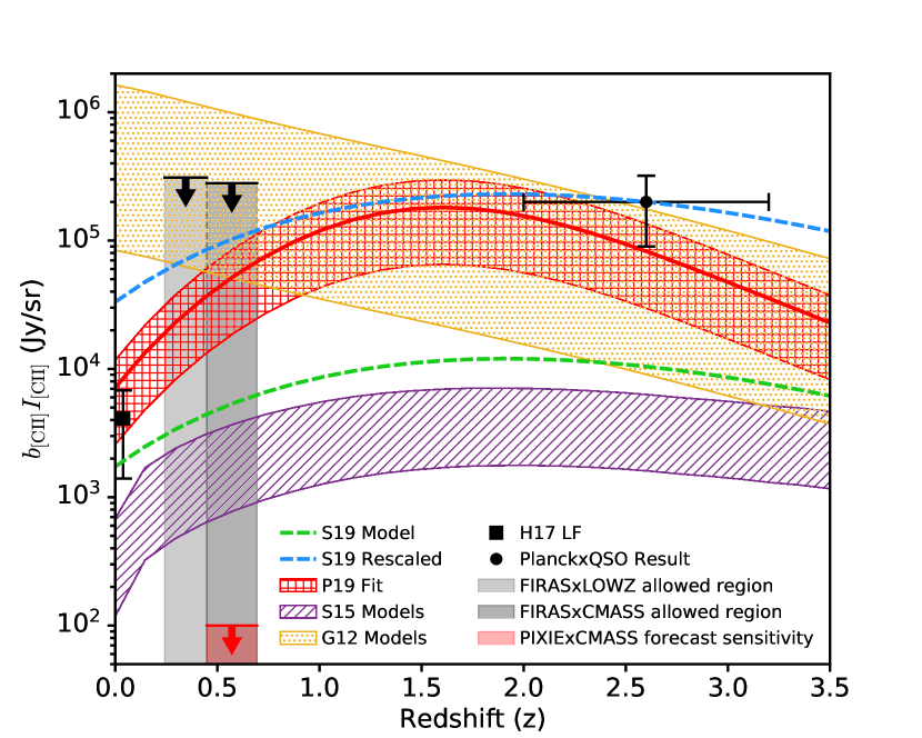
Figure 13 compares FIRASBOSS upper limits on to several representative physical models of [C II] brightness as a function of redshift. It also shows the PlanckQSO intensity mapping constraint from Yang et al. (2019), assuming that the excess power detected is [C II] emission. Models that do not scale [C II] emission with star formation rate evolution are disfavored because their low-redshift [C II] emission is too bright. Models that scale [C II] emission with star formation rate can be calibrated with physical parameters to be consistent with both FIRASBOSS and PlanckQSO.
The yellow dotted region in Figure 13 shows the range of [C II] amplitudes predicted by the collisional excitation model from Gong et al. (2012), hereafter G12. In this model, the mean [C II] intensity is computed through a simple radiative transfer model whose free parameters are the number density and kinetic temperature of electrons within the emitting galaxies. The yellow dotted region spans the range of and values considered by G12. Because this model predicts comparatively bright [C II] emission, Yang et al. (2019) argue that it provides the best-fit to their measurement and use their result to place constraints on the two free parameters. FIRASBOSS upper limits at rule out the brightest range of the G12 predictions. Since it is this bright end that is consistent with the Yang et al. (2019) measurement at , the G12 model is disfavored to explain the FIRASBOSS and PlanckQSO [C II] measurements.
The G12 model was originally created to forecast emission at much higher redshifts, during the epoch of reionization. Since [C II] luminosity is expected to be correlated with star formation, we qualitatively expect the [C II] amplitude to follow the cosmic star formation history and come to a peak around , declining to the present day (Madau & Dickinson, 2014). This is not seen in the G12 model, which monotonically increases as we move to lower redshift. Thus the bright G12 predictions, which are disfavored by the combination of FIRASBOSS and PlanckQSO, may not be a physically accurate estimate of the true [C II] evolution during more recent epochs since .
Next, we consider the scaling models from Silva et al. (2015) (hereafter S15), shown as the hatched purple region in Figure 13. Silva et al. (2015) consider four different empirically-calibrated power-law scaling relations between [C II] luminosity and star formation rate (SFR). The hatched purple region shows the full range of [C II] luminosity predictions from the four values of the slope and amplitude of this power-law scaling from their Table 1. Although these models were originally constructed to predict [C II] intensity at reionization redshifts, they are correlated with the cosmic star formation history and thus show the qualitative redshift evolution we expect, with a peak at and a decline at lower redshifts. These predictions fall a factor of 100 or more below our FIRASBOSS upper limits at , putting them well below our ability to constrain. However, these models also fall well below the PlanckQSO estimate, meaning they may also be pessimistic predictions.
Next, we examine the “semi-empirical" model from Sun et al. (2019) (hereafter S19), plotted as a dashed green curve. This calculation falls somewhat between the other two. It uses a physically motivated scaling between the [C II] and infrared luminosity of a halo. This scaling is parameterized in terms of the photoelectric heating efficiency from dust grains, . The distribution of galaxy infrared luminosities is calibrated to empirical measurements of the cosmic infrared background (Planck Collaboration et al., 2014b). This model also predicts a fiducial [C II] amplitude well below our limits and the Yang et al. (2019) measurement. However, as shown in Figure 10 of S19, the [C II] intensity can be brought into agreement with the PlanckQSO measurement, if one increases by a factor of from their fiducial number. The authors, however, note that this higher value may lead to tension with the observed relation between [C II] luminosity and star formation rate in low-redshift galaxies. The redshift evolution of this rescaled S19 model is plotted as the dashed blue curve in Figure 13. In contrast with the G12 model, we find that our FIRAS measurements are fully consistent with the redshift evolution seen here, even scaling to the brighter emission at suggested by Yang et al. (2019).
We also include, in red, an empirical fit from Padmanabhan (2019) (hereafter P19), which uses the technique of abundance-matching to fit a power-law luminosity function with an exponential cut-off to the measured [C II] luminosity function from Hemmati et al. (2017). The amplitude of [C II] emission in P19 evolves with redshift as a power-law of the observed star-formation rate density, whose redshift evolution was measured by Madau & Dickinson (2014). The power-law index is fit to be consistent with the value reported by Pullen et al. (2018) at . In order to accommodate this large increase in intensity from to , the best-fit value for this index is . This is substantially higher than the values near unity assumed in S15 (Silva et al., 2015), based on observations of individual local and high-redshift galaxies. The hatched red region shows the range for the P19 model fits, and the solid red line is the best-fit model. Because the P19 fit finds a lower mass range for [C II] emitters than that assumed in the model of Pullen et al. (2018), it has a lower value for , and consequently, a lower value for at .
Figure 13 also includes a point at from the luminosity function measurements of Hemmati et al. (2017), which integrates to kJy/sr. The measured galaxies cover the to solar luminosity range, via a mix of direct detection of [C II] emission, at the bright end, and inference of [C II] emission via FIR brightness and color measurements, at the dim end. An integral of this luminosity function yields the expected [C II] brightness, , but in order to plot , a model for the [C II] bias must be assumed. We estimate a bias of 1, which corresponds to the value from the halo model used in appendix B. This roughly matches the bias evolution of all the models plotted, which predict decreasing bias at low redshift. This convergence of bias toward unity at low redshift occurs because, as halo masses increase at low redshift, the mass range for [C II]-hosting galaxies becomes less biased towards the higher mass end of the halo distribution.
The models that calibrate the [C II]-SFR relationship based on observations of known galaxies (S15) or on simple physical mechanisms (S19) struggle to decrease quickly enough at low redshift to be consistent with both PlanckQSO and Hemmati et al. (2017). Assuming that the PlanckQSO excess is [C II] emission, there are still several possible explanations. The estimated [C II] bias of 1 could be too low. However, the required bias of 8 to bring Hemmati et al. (2017) to agreement with the re-scaled S19 model would be extremely large compared to biases typically inferred from these [C II] models. Alternatively, there could be an undetected population of low-luminosity [C II] galaxies. In fact, Hemmati et al. (2017) suggest the possibility of unmeasured faint low-metallicity dwarf-galaxies, which would have a different [C II]-FIR calibration, contributing to the faint end of the [C II] luminosity function. This possibility highlights a trend where early intensity mapping results suggest unexpectedly bright cumulative emission compared to direct detection of individual objects. For instance, Breysse et al. (2021a) suggests that potential bright CO emission detected by mmIME (Keating et al., 2020) may be due to a large population of dim CO galaxies. Indeed, this CO excess is of a similar order of magnitude to the difference seen here between the S19 and PlanckQSO [C II] values, hinting at a possibly related cause. Another possibility is that the assumption of these models, that [C II] emission is directly tied to the star formation rate, is too simple.
Conclusions here are limited by thermal noise in FIRAS. To meaningfully constrain the space of models, qualitatively new improvements in sensitivity are required. To put FIRAS in the context of what could be achieved by a modern mission, we compute the potential sensitivity achievable by cross-correlating maps from the proposed PIXIE satellite with the CMASS galaxy maps used in this paper. The Primordial Inflation Explorer (PIXIE) is a proposed NASA Explorer-class mission to measure the polarized imprint of primordial inflation on the CMB (Kogut et al., 2011), along with several other spectral distortions of the CMB (Chluba et al., 2021). PIXIE will conduct an all-sky survey with angular and spectral resolution and spectral coverage similar to FIRAS. However, the beam will be slightly smaller, and the noise level will be three orders of magnitude lower than FIRAS. These properties make PIXIE well-placed to study star-formation and scale-dependent bias as a test of non-Gaussianity via intensity mapping (Dizgah et al., 2019; Switzer, 2017b).
To assess PIXIE’s constraining power, we conduct a suite of 10,000 simulations with no [C II] signal. These simulations project that a cross-correlation of PIXIE maps with CMASS galaxies could place an upper limit of Jy/sr on at confidence (see the red transparent region in Figure 13). This result means that PIXIECMASS is easily sensitive enough to detect even the most pessimistic [C II] models at high significance.
In addition to PIXIE, many of the other planned or in-progress intensity mapping surveys described in Section 1 could shed useful light on the redshfit evolution of the [C II] line. The TIM and EXCLAIM surveys will produce maps of [C II] at redshifts and respectively, with considerably more sensitivity than FIRAS and better spectral resolution than Planck. Parallel measurements of CO emission over similar redshift range, though they track somewhat different ISM physics, are still strongly correlated with star formation and will be quite complementary to the [C II] measurments. The COMAP survey has produced early science limits on CO(1-0) emission in a similar redshift range to the PlanckQSO [C II] observation, and should have sufficient sensitivity to explore these discrepancies with their full data set (Chung et al., 2021; Breysse et al., 2021b). Similarly, though the TIME, CONCERTO, and FYST surveys primarily target reionization-era lines, they have several CO “foregrounds" which would overlap with the FIRAS redshift range, potentially enabling deeper measurements.
6 Conclusion
Our analysis constrains the product of the bias and specific intensity of [C II], , to be MJy/sr at and MJy/sr at at confidence. Through both FIRAS’ unique capability for tomographic measurement and the depth of BOSS data at these redshifts, bounds on [C II] developed here are competitive with those achieved in the recent analysis of Planck data (Yang et al., 2019; Pullen et al., 2018). We rule out a swath of collisional excitation models consistent with PlanckQSO, but note that those models were not designed to predict low redshift [C II]. [C II] emission is expected to correlate with the star formation rate, which appears to have peaked at and then declined at later redshifts (Madau & Dickinson, 2014). Our constraints are consistent with all models that include this expected correlation of [C II] emission with star formation rate. If the high [C II] intensity measured from PlanckQSO is accurate, then [C II] models with realistic redshift evolution tied to the star formation rate predict MJy/sr at . This expected value is nearly within reach of the FIRAS data. Measurements described here are limited by FIRAS thermal noise and angular resolution rather than the depth of the galaxy redshift survey, so substantial further progress will require new intensity mapping measurements. We show that the proposed PIXIE mission could detect even pessimistic models for [C II] emission. The SHT approach developed here also applies well to wide-field surveys such as HIRAX, CHIME, TianLai, HERA, and SPHEREx, both in auto-power and crosspower. The SHT is broadly well-matched to intensity mapping analysis through its ability to capture all Gaussian information directly in observed map space and to easily account for survey effects such as the curved sky and inhomogeneous noise.
Acknowledgements
We would like to thank Dale Fixsen, Nathan Miller, and Nils Odegard for their useful input regarding the FIRAS noise and beam model. Some of the results in this paper have been derived using the healpy and HEALPix package. PCB was supported by the James Arthur Postdoctoral Fellowship.
Funding for the Sloan Digital Sky Survey IV has been provided by the Alfred P. Sloan Foundation, the U.S. Department of Energy Office of Science, and the Participating Institutions. SDSS-IV acknowledges support and resources from the Center for High Performance Computing at the University of Utah. The SDSS website is www.sdss.org.
SDSS-IV is managed by the Astrophysical Research Consortium for the Participating Institutions of the SDSS Collaboration including the Brazilian Participation Group, the Carnegie Institution for Science, Carnegie Mellon University, Center for Astrophysics | Harvard & Smithsonian, the Chilean Participation Group, the French Participation Group, Instituto de Astrofísica de Canarias, The Johns Hopkins University, Kavli Institute for the Physics and Mathematics of the Universe (IPMU) / University of Tokyo, the Korean Participation Group, Lawrence Berkeley National Laboratory, Leibniz Institut für Astrophysik Potsdam (AIP), Max-Planck-Institut für Astronomie (MPIA Heidelberg), Max-Planck-Institut für Astrophysik (MPA Garching), Max-Planck-Institut für Extraterrestrische Physik (MPE), National Astronomical Observatories of China, New Mexico State University, New York University, University of Notre Dame, Observatário Nacional / MCTI, The Ohio State University, Pennsylvania State University, Shanghai Astronomical Observatory, United Kingdom Participation Group, Universidad Nacional Autónoma de México, University of Arizona, University of Colorado Boulder, University of Oxford, University of Portsmouth, University of Utah, University of Virginia, University of Washington, University of Wisconsin, Vanderbilt University, and Yale University.
Data Availability
The FIRAS data underlying these results are available on NASA’s LAMBDA archive at https://lambda.gsfc.nasa.gov/product/cobe/firas_prod_table.cfm. The BOSS data underlying these results are on the BOSS data release 12 archive at https://www.sdss.org/dr12/.
Appendix A Cross-power Approximate Sensitivity Forecast
The complete tomographic likelihood for has a complex structure. This appendix simplifies the sensitivity to its essential elements to provide some intuition. For a survey where the intensity map auto-power is noise and/or foreground dominated, the covariance on the cross-power along the angular diagonal () is roughly
| (23) |
FIRAS lacks the redshift resolution for there to be a significant signal in the [C II] or galaxy angular cross-power when . Considering only cross-correlations between the same redshift slice, the covariance is zero except along the redshift diagonal . We also assume that the bandpowers are broad enough to have negligible correlations for . Dropping redshift subscripts, the binned [C II] cross-power signal can be modeled as , where is the binned dark matter angular power spectrum, is the bias of [C II] galaxies, and is the specific intensity of [C II] emission. From this signal model and Equation 23, the variance on a determination of from the angular cross-power of any single redshift and an angular bin is 222An interesting feature of this formula is that, for a wide range of redshift bin sizes, this variance on the line amplitude is roughly the same. For instance, if FIRAS had half of its actual redshift resolution, the cosmological and galaxy clustering power spectrum would wash out by a factor of 1/2, but the increased bandwidth would also decrease the thermal noise signal in the FIRAS auto-power spectrum by 1/2. These effects would cancel out to keep the variance per angular bin and redshift slice constant.
| (24) |
The total constraining power is an inverse variance weighted sum over the angular and redshift bins,
| (25) |
From this formula, we predict a sensitivity of 0.27 MJy/sr () on . In computing this estimate, we have neglected foregrounds and assumed that only thermal noise contributes to , since smooth foregrounds are de-weighted with only a small penalty to sensitivity. This simple estimate closely matches the precision we achieve with the complete calculation.
Appendix B Details of model for FIRASBOSS
To model the dust and [C II] emission, we employ a technique similar to Pullen et al. (2018). Using the halo model, the redshift distribution of specific intensity is
| (26) |
where represents the redshifted specific luminosity for a halo of mass , given by , where represents the rest-frame specific luminosity evaluated at . On the second line of Equation 26, we introduced the mean comoving emission coefficient , defined as
| (27) |
Following the analysis of extragalactic cosmic infrared background (CIB) emission of Shang et al. (2012), the specific luminosity is parameterized as
| (28) |
where is a normalization constant, parameterizes the mass dependence of the halo luminosity, and parameterizes the redshift evolution of both the continuum and [C II] luminosity, which we assume evolve together. is expected to have peaked around (Madau & Dickinson, 2014). A sufficiently precise intensity mapping experiment with a large frequency bandwidth can, in principle, constrain the form of the redshift dependence of . FIRASBOSS, however, lacks the precision to measure this evolution, so we choose to model it with a simple power-law, , following the parameterization and fit of Pullen et al. (2018). is assumed to follow a log-normal distribution
| (29) |
where (Planck Collaboration et al., 2014b; Serra et al., 2016) and (Shang et al., 2012; Planck Collaboration et al., 2014b; Serra et al., 2016). The integral over the halo mass function is computed with the python package hmf (Murray, 2014), assuming Planck 2015 (Ade et al., 2016) cosmological parameters and a Tinker et al. (2008) functional form for . We include [C II] emission in this specific luminosity by assuming that each CIB galaxy emits continuum emission and a narrow [C II] line. Assuming that the ratio of total power emitted by the line and the continuum is constant, and ignoring the finite mass-dependent velocity width of the galaxy, we parameterize as the sum of continuum emission (, parametric form from Shang et al. (2012)) and [C II] line emission
| (30) |
where we have defined to be the ratio of the total power of the continuum emission to the total power of [C II] line emission. We choose , in agreement with Planck Collaboration et al. (2014a). Serra et al. (2014b) measured the dust temperature of the BOSS CIB to be 26 K, which means all of the CIB emission in the FIRAS frequencies of this analysis is below the turnover frequency , so only the semi-thermal form of is used.
The FIRAS instrument measures the average intensity in a given frequency bin. Ignoring redshift space distortions and any contributions from thermal noise and Milky Way foregrounds, the observed intensity is given by
| (31) |
where we have explicitly separated the continuum and [C II] contributions. We do this because the cross-correlation signal between FIRAS and BOSS has two components: (1) a galaxy-[C II] cross-correlation component with narrow redshift window functions for both the optical galaxies and the [C II] sources, and (2) a galaxy-continuum component with a narrow redshift window function for the optical galaxies but a broad redshift window function, given by , for the CIB continuum:
| (32) |
The angular power spectrum between signal types and is given by
| (33) |
where (ignoring RSD for now, and using equations 26 through 31 for the [C II] and CIB signals) the Window functions for optical galaxies, [C II], and continuum emission are as follows:
| (34) |
where is the growth factor and and are set by the spectral channels of FIRAS for . As stated in Section 3.2, the galaxy window function was chosen to have the same and as the FIRAS spectral channels.
If we make the reasonable approximation that all -dependent quantities of the dust and [C II] model vary slowly within the redshift bins determined by the FIRAS frequency channels, then we can compute and fully, including linear redshift space distortions, in terms of , , and , which were defined in Section 4.1. For , we have
| (35) |
where
| (36) |
In Equation 36, we have used . The [C II] intensity has a redshift dependence, determined by both cosmological factors and the assumed specific luminosity parameterization of Equation 28. They lead to a [C II] intensity that increases by a factor of about 20 percent over each of the CMASS and LOWZ redshift ranges. In our analysis, the shape of this redshift evolution is fixed, and we fit only for the overall amplitude of . We calculate the CIB signal in a similar manner, as
| (37) |
where is the intensity of the CIB that is emitted from sources in a redshift bin of size , centered at redshift , and measured at a frequency of . Assuming the CIB spectrum does not change significantly within the FIRAS frequency bin, then is
| (38) |
The sum over in Equation 37 should, in principle, be carried out over all redshifts, even those outside of the galaxy survey. In practice, for the redshift bins and bins considered in this analysis, the bracketed kernel is dominated by the term, with the neighboring off-diagonal terms around 20% of the diagonal term, and the rest of the terms are negligible. Analogously to our [C II] analysis, we do not attempt to constrain the redshift evolution of the CIB brightness or the spectral shape of the CIB emission. Instead, these are fixed by the assumed values of , K, , , and . Because of this assumed spectral and redshift evolution, the parameter that we fit for is only the exact continuum intensity per unit redshift at , the central redshift of the survey, and , the central frequency of the survey.
Equations 35 and 37 show how high spectral resolution allows a separation of correlated line and continuum emission in intensity mapping. In the limit where the spectral resolution is very low and is high, all the off-diagonal terms of are zero, collapsing the sum of Equation 37 to only the term. Dividing the [C II] signal by the CIB signal, one finds that the ratio of [C II] to CIB cross-power scales as (this point is subtle because one is free to choose to be an arbitrarily small value in Equation 37, but the redshift window for Equation 35 is fixed by the spectral resolution of the intensity mapping survey. Therefore, one can choose the same redshift window for the CIB calculation so that the terms cancel.). This simple scaling, where higher redshift resolution continues to linearly improve the ability to distinguish line emission from continuum emission, remains true until the redshift resolution is high enough to resolve off-diagonal components of .
Appendix C Covariance angular coupling approximation
This section reviews a formula for approximating the coupling in the covariance. The formula comes directly from the work of Tristram et al. (2005), originally developed for pseudo- cross-correlation studies of CMB maps from different instruments or different detectors of the same instrument. We use the notation of Section 2, where unbinned quantities retain the subscript, and binned quantities are written with the subscript . Let represent the binned angular power spectrum between maps of type and type , where and can represent different redshifts or different types of maps (intensity maps or binned galaxy surveys). Then, the covariance can be written
| (39) |
where represents the inverse of the binned mixing matrix between maps and , defined by equations 2 and 3, and where is the covariance of the pseudo-, given by
| (40) |
In the above formula, is a binning matrix, is the combined beam and pixel window function for map (and analogously for maps , and ), and is the cross-correlation matrix, defined by
| (41) |
where
| (42) |
In the above formula, represents a spherical harmonic coefficient of the inverse noise weights for map .
The covariance presented in this section uses an approximation that works best when the sky coverage is large. We find it sufficient for our BOSSBOSS analysis, but for FIRASFIRAS and FIRASBOSS, the formula appears to be inaccurate, possibly due to the combination of the steep angular index on the foregrounds combined with the small sky fraction. We instead use a simulated covariance for FIRASFIRAS and FIRASBOSS.
Appendix D Updating the covariance for FIRASBOSS
We calculate a simulated covariance by drawing individual amplitudes from our FIRAS foregrounds plus noise model, cosmological signal model, and galaxy shot noise model. Each of these models is assumed to be Gaussian and uncorrelated. We then compute simulated full-sky galaxy maps from the sum of the cosmological and shot noise draws. We also compute simulated full-sky FIRAS maps from the sum of the foreground and noise realization plus a painting of [C II] and CIB signal onto the cosmological signal realization. The simulated FIRAS signal is then convolved with the FIRAS beam, scan, and pixel window function. Then, the simulated FIRAS and BOSS maps are multiplied by their respective weights, and the cross-power spectrum between the FIRAS and BOSS maps is computed. A simulated covariance is calculated from 10,000 of these realizations. This procedure assumes a specific value for the [C II] and CIB brightness, but the covariance should change as the [C II] and CIB magnitude change. So, we use four sets of simulations to create a simulated covariance that correctly updates its [C II] and CIB contribution to match the current [C II] and CIB magnitude estimates.
From the assumption of Gaussian power spectra, the rough form of the FIRASBOSS covariance is
| (43) |
where the partial sky also introduces some level of coupling between different angular bins, which we compute via our simulations. Schematically, dropping the redshift indices, the two terms in brackets can be broken down as follows.
| (44) |
| (45) |
where refers to the model of Milky Way foregrounds plus noise. Due to the large foregrounds and noise, the magnitude of the covariance is dominated by the term. However, we find that the best-fit values for and are somewhat affected by the values one assumes for them in the covariance model, so we need to be able to vary their magnitude in our covariance model. This requires four simulations, which we describe in table 1.
| Simulated Covariances | ||||
|---|---|---|---|---|
| Name | FG, Noise Amplitude | |||
| FIRASFIRAS best-fit | 0 | 0 | BOSSBOSS best-fit | |
| 0 | 1 | 0 | BOSSBOSS best-fit | |
| 0 | 0 | 1 | BOSSBOSS best-fit | |
| 0 | 1 | 1 | BOSSBOSS best-fit | |
These four simulations give the following approximate covariances:
| (46) |
| (47) |
| (48) |
| (49) |
From the bottom three simulations, we can isolate the term that arises due to cross-correlations between [C II] and CIB, as follows:
| (50) |
The total covariance for arbitrary [C II] and CIB amplitudes can now be constructed as follows:
| (51) |
This is the covariance used for our cross-power estimator in Section 4.2 and in our FIRAS validation simulations, described in Appendix E.
Appendix E Validating the parametric FIRAS model in the covariance for FIRASBOSS
We compare two sets of simulations, each performed over both the CMASS and LOWZ regions. In the first set of simulations, we draw the FIRAS amplitudes from the parametric model fit described in Section 4.3.3. In the second set of simulations, the FIRAS amplitudes are drawn from an empirical FIRAS model that is the measured FIRAS auto-power in bandpowers. In all cases, the BOSS signal is drawn from the parametric fit of Section 4.3.2, and both the [C II] and CIB amplitudes are set to zero. We draw 10,000 realizations for each set of simulations and compute the covariance directly from the simulations. We then find the maximum likelihood solution for each realization, using a Gaussian likelihood with this simulated covariance (and also updating the covariance to account for the current [C II] and CIB estimate according to Equation 51). Note that the empirical FIRAS-model simulations are not subject to cosmic bias because the real [C II] and CIB signal present in the empirical FIRAS model is not correlated with the simulated cosmological clustering realization. Figure 14 shows that the empirical (blue) and parametric (red) FIRAS simulations lead to near-identical uncertainties on and .

As a consistency check on our MCMC procedure, we also perform an MCMC analysis on one of our realizations for the parametric covariance. We verify that the 95 and 68 percent MCMC contours are nearly identical in size and shape to the 95 and 68 percent contours of the histogram of maximum likelihood points from our 10,000 simulations. This calculation confirms that the parametric variance model for FIRASFIRAS yield errors consistent with those inferred from the measured FIRASFIRAS power spectrum (that the parametric FIRASFIRAS model is sufficiently accurate).
References
- Abdalla et al. (2021) Abdalla E., et al., 2021, arXiv e-prints, p. arXiv:2107.01633
- Abramo et al. (2016) Abramo L. R., Secco L. F., Loureiro A., 2016, MNRAS, 455, 3871
- Ade et al. (2016) Ade P. A. R., et al., 2016, Astronomy & Astrophysics, 594, A13
- Alam et al. (2015) Alam S., et al., 2015, The Astrophysical Journal Supplement Series, 219, 12
- Alonso (2018) Alonso D., 2018, NaMaster github, https://github.com/LSSTDESC/NaMaster
- Alonso et al. (2019) Alonso D., Sanchez J., Slosar A., 2019, Monthly Notices of the Royal Astronomical Society, 484, 4127
- Anderson et al. (2018) Anderson C. J., et al., 2018, Monthly Notices of the Royal Astronomical Society, 476, 3382
- Asorey et al. (2012) Asorey J., Crocce M., Gaztañaga E., Lewis A., 2012, Monthly Notices of the Royal Astronomical Society, 427, 1891
- Balaguera-Antolínez et al. (2018) Balaguera-Antolínez A., Bilicki M., Branchini E., Postiglione A., 2018, MNRAS, 476, 1050
- Bandura et al. (2014) Bandura K., et al., 2014, in Stepp L. M., Gilmozzi R., Hall H. J., eds, Society of Photo-Optical Instrumentation Engineers (SPIE) Conference Series Vol. 9145, Ground-based and Airborne Telescopes V. p. 914522 (arXiv:1406.2288), doi:10.1117/12.2054950
- Breysse et al. (2021a) Breysse P. C., Yang S., Somerville R. S., Pullen A. R., Popping G., Maniyar A. S., 2021a, arXiv e-prints, p. arXiv:2106.14904
- Breysse et al. (2021b) Breysse P. C., et al., 2021b, arXiv e-prints, p. arXiv:2111.05933
- Bull et al. (2015) Bull P., Ferreira P. G., Patel P., Santos M. G., 2015, The Astrophysical Journal, 803, 21
- CCAT-Prime collaboration et al. (2021) CCAT-Prime collaboration et al., 2021, arXiv e-prints, p. arXiv:2107.10364
- Campagne et al. (2017) Campagne J. E., Neveu J., Plaszczynski S., 2017, Astronomy & Astrophysics, 602, A72
- Carilli & Walter (2013) Carilli C. L., Walter F., 2013, Annual Review of Astronomy and Astrophysics, 51, 105
- Cataldo et al. (2021) Cataldo G., et al., 2021, arXiv e-prints, p. arXiv:2101.11734
- Chang et al. (2008) Chang T.-C., Pen U.-L., Peterson J. B., McDonald P., 2008, Physical Review Letters, 100, 091303
- Chang et al. (2010) Chang T.-C., Pen U.-L., Bandura K., Peterson J. B., 2010, Nature, 466, 463
- Chen (2012) Chen X., 2012, in International Journal of Modern Physics Conference Series. pp 256–263 (arXiv:1212.6278), doi:10.1142/S2010194512006459
- Cheng et al. (2018) Cheng C., et al., 2018, The Astrophysical Journal, 868, 26
- Chluba et al. (2021) Chluba J., et al., 2021, Experimental Astronomy, pp 1–40
- Chung et al. (2021) Chung D. T., et al., 2021, arXiv e-prints, p. arXiv:2111.05931
- Cleary et al. (2021) Cleary K. A., et al., 2021, arXiv e-prints, p. arXiv:2111.05927
- Crichton et al. (2021) Crichton D., et al., 2021, arXiv e-prints, p. arXiv:2109.13755
- Crites et al. (2014) Crites A. T., et al., 2014, in Holland W. S., Zmuidzinas J., eds, Society of Photo-Optical Instrumentation Engineers (SPIE) Conference Series Vol. 9153, Millimeter, Submillimeter, and Far-Infrared Detectors and Instrumentation for Astronomy VII. p. 91531W, doi:10.1117/12.2057207
- Dawson et al. (2012) Dawson K. S., et al., 2012, The Astronomical Journal, 145, 10
- DeBoer et al. (2017) DeBoer D. R., et al., 2017, Publications of the Astronomical Society of the Pacific, 129, 045001
- Di Dio et al. (2013) Di Dio E., Montanari F., Lesgourgues J., Durrer R., 2013, Journal of Cosmology and Astroparticle Physics, 2013, 044
- Di Dio et al. (2014) Di Dio E., Montanari F., Durrer R., Lesgourgues J., 2014, Annual Review of Astronomy and Astrophysics, 2014, 042
- Díaz-Santos et al. (2017) Díaz-Santos T., et al., 2017, American Astronomical Society, 846, 32
- Dizgah et al. (2019) Dizgah A. M., Keating G. K., Fialkov A., 2019, The Astrophysical Journal Letters, 870, L4
- Doi et al. (2010) Doi M., et al., 2010, The Astronomical Journal, 139, 1628
- FIRAS Collaboration (1997) FIRAS Collaboration 1997, FIRAS Explanatory Supplement, https://lambda.gsfc.nasa.gov/product/cobe/firas_exsupv4.cfm
- Fisher et al. (1994) Fisher K. B., Scharf C. A., Lahav O., 1994, Monthly Notices of the Royal Astronomical Society, 266, 219
- Fisher et al. (1995) Fisher K. B., Lahav O., Hoffman Y., Lynden-Bell D., Zaroubi S., 1995, MNRAS, 272, 885
- Fixsen et al. (1994) Fixsen D., et al., 1994, The Astrophysical Journal, 420, 457
- Fixsen et al. (1999) Fixsen D. J., Bennett C., Mather J. C., 1999, The Astrophysical Journal, 526, 207
- Fonseca et al. (2019) Fonseca J., Viljoen J.-A., Maartens R., 2019, J. Cosmology Astropart. Phys., 2019, 028
- Fukugita et al. (1996) Fukugita M., Ichikawa T., Gunn J. E., Doi M., Shimasaku K., Schneider D. P., 1996, The Astronomical Journal, 111, 1748
- Gong et al. (2012) Gong Y., Cooray A., Silva M., Santos M. G., Bock J., Bradford C. M., Zemcov M., 2012, The Astrophysical Journal, 745, 49
- Gong et al. (2017) Gong Y., Cooray A., Silva M. B., Zemcov M., Feng C., Santos M. G., Dore O., Chen X., 2017, The Astrophysical Journal, 835, 273
- Górski et al. (2005) Górski K. M., Hivon E., Banday A. J., Wandelt B. D., Hansen F. K., Reinecke M., Bartelmann M., 2005, The Astrophysical Journal, 622, 759
- Grasshorn Gebhardt & Doré (2021) Grasshorn Gebhardt H. S., Doré O., 2021, Phys. Rev. D, 104, 123548
- Grasshorn Gebhardt & Jeong (2020) Grasshorn Gebhardt H. S., Jeong D., 2020, Phys. Rev. D, 102, 083521
- Gunn et al. (1998) Gunn J. E., et al., 1998, The Astronomical Journal, 116, 3040
- Gunn et al. (2006) Gunn J. E., et al., 2006, The Astronomical Journal, 131, 2332
- Guo et al. (2015) Guo H., et al., 2015, Monthly Notices of the Royal Astronomical Society, 446, 578
- Hamimeche & Lewis (2008) Hamimeche S., Lewis A., 2008, Physical Review D, 77, 103013
- Heavens & Taylor (1995) Heavens A. F., Taylor A. N., 1995, MNRAS, 275, 483
- Hemmati et al. (2017) Hemmati S., Yan L., Diaz-Santos T., Armus L., Capak P., Faisst A., Masters D., 2017, The Astrophysical Journal, 834, 36
- Hivon et al. (2002) Hivon E., Górski K. M., Netterfield C. B., Crill B. P., Prunet S., Hansen F., 2002, The Astrophysical Journal, 567, 2
- Hogan & Rees (1979) Hogan C. J., Rees M. J., 1979, Monthly Notices of the Royal Astronomical Society, 188, 791
- Karkare et al. (2022) Karkare K. S., et al., 2022, Journal of Low Temperature Physics,
- Keating et al. (2016) Keating G. K., Marrone D. P., Bower G. C., Leitch E., Carlstrom J. E., DeBoer D. R., 2016, The Astrophysical Journal, 830, 34
- Keating et al. (2020) Keating G. K., Marrone D. P., Bower G. C., Keenan R. P., 2020, The Astrophysical Journal, 901, 141
- Keenan et al. (2021) Keenan R. P., Keating G. K., Marrone D. P., 2021, arXiv e-prints, p. arXiv:2110.02239
- Kogut et al. (2011) Kogut A., et al., 2011, Journal of Cosmology and Astroparticle Physics, 2011, 025
- Kovetz et al. (2017) Kovetz E. D., et al., 2017, arXiv preprint arXiv:1709.09066
- Kovetz et al. (2019) Kovetz E., et al., 2019, Bulletin of the American Astronomical Society
- Lanusse et al. (2015) Lanusse F., Rassat A., Starck J. L., 2015, Astronomy & Astrophysics, 578, A10
- Leistedt et al. (2012) Leistedt B., Rassat A., Réfrégier A., Starck J. L., 2012, A&A, 540, A60
- Leistedt et al. (2013) Leistedt B., Peiris H. V., Mortlock D. J., Benoit-Lévy A., Pontzen A., 2013, MNRAS, 435, 1857
- Lewis & Challinor (2011) Lewis A., Challinor A., 2011, CAMB: Code for Anisotropies in the Microwave Background (ascl:1102.026)
- Liu et al. (2016) Liu A., Zhang Y., Parsons A. R., 2016, The Astrophysical Journal, 833, 242
- Liu et al. (2017) Liu H., von Hausegger S., Naselsky P., 2017, Physical Review D, 95, 103517
- Loureiro et al. (2019a) Loureiro A., et al., 2019a, Monthly Notices of the Royal Astronomical Society, 485, 326
- Loureiro et al. (2019b) Loureiro A., et al., 2019b, Monthly Notices of the Royal Astronomical Society, 485, 326
- Madau & Dickinson (2014) Madau P., Dickinson M., 2014, Annual Review of Astronomy and Astrophysics, 52, 415
- Madau et al. (1997) Madau P., Meiksin A., Rees M. J., 1997, The Astrophysical Journal, 475, 429
- Malhotra et al. (1997) Malhotra S., et al., 1997, The Astrophysical Journal Letters, 491, L27
- Masui et al. (2013) Masui K. W., et al., 2013, The Astrophysical Journal Letters, 763, L20
- Mather et al. (1993) Mather J. C., Fixsen D. J., Shafer R. A., 1993, in Infrared Spaceborne Remote Sensing. pp 168–180
- McDonald & Seljak (2009) McDonald P., Seljak U., 2009, Journal of Cosmology and Astroparticle Physics, 10, 007
- McKinley et al. (2018) McKinley B., et al., 2018, Monthly Notices of the Royal Astronomical Society, 481, 5034
- Mondal et al. (2018) Mondal R., Bharadwaj S., Datta K. K., 2018, MNRAS, 474, 1390
- Mondal et al. (2019) Mondal R., Bharadwaj S., Iliev I. T., Datta K. K., Majumdar S., Shaw A. K., Sarkar A. K., 2019, MNRAS, 483, L109
- Mondal et al. (2020) Mondal R., Shaw A. K., Iliev I. T., Bharadwaj S., Datta K. K., Majumdar S., Sarkar A. K., Dixon K. L., 2020, MNRAS, 494, 4043
- Mondal et al. (2022) Mondal R., Mellema G., Murray S. G., Greig B., 2022, arXiv e-prints, p. arXiv:2203.11095
- Murray (2014) Murray S., 2014, HMF: Halo Mass Function calculator (ascl:1412.006)
- Nicola et al. (2014) Nicola A., Refregier A., Amara A., Paranjape A., 2014, Physical Review D, 90, 063515
- Nicola et al. (2020) Nicola A., et al., 2020, J. Cosmology Astropart. Phys., 2020, 044
- Oxholm & Switzer (2021) Oxholm T. M., Switzer E. R., 2021, Physical Review D, 104, 083501
- Padmanabhan (2019) Padmanabhan H., 2019, MNRAS, 488, 3014
- Padmanabhan et al. (2007) Padmanabhan N., et al., 2007, Monthly Notices of the Royal Astronomical Society, 378, 852
- Pen et al. (2009) Pen U.-L., Staveley-Smith L., Peterson J. B., Chang T.-C., 2009, Monthly Notices of the Royal Astronomical Society, 394, L6
- Planck Collaboration et al. (2014a) Planck Collaboration et al., 2014a, Astronomy & Astrophysics, 566, A55
- Planck Collaboration et al. (2014b) Planck Collaboration et al., 2014b, Astronomy & Astrophysics, 571, A30
- Popping et al. (2019) Popping G., Narayanan D., Somerville R. S., Faisst A. L., Krumholz M. R., 2019, Monthly Notices of the Royal Astronomical Society, 482, 4906
- Pullen et al. (2018) Pullen A. R., Serra P., Chang T.-C., Doré O., Ho S., 2018, Monthly Notices of the Royal Astronomical Society, 478, 1911
- Rassat & Refregier (2012) Rassat A., Refregier A., 2012, A&A, 540, A115
- Salazar-Albornoz et al. (2017) Salazar-Albornoz S., et al., 2017, Monthly Notices of the Royal Astronomical Society, 468, 2938
- Schöneberg et al. (2018) Schöneberg N., Simonović M., Lesgourgues J., Zaldarriaga M., 2018, Journal of Cosmology and Astroparticle Physics, 10, 047
- Scott & Rees (1990) Scott D., Rees M. J., 1990, Monthly Notices of the Royal Astronomical Society, 247, 510
- Serra et al. (2014a) Serra P., Lagache G., Doré O., Pullen A., White M., 2014a, Astronomy & Astrophysics, 570, A98
- Serra et al. (2014b) Serra P., Lagache G., Doré O., Pullen A., White M., 2014b, Astronomy & Astrophysics, 570, A98
- Serra et al. (2016) Serra P., Doré O., Lagache G., 2016, The Astrophysical Journal, 833, 153
- Shang et al. (2012) Shang C., Haiman Z., Knox L., Oh S. P., 2012, Monthly Notices of the Royal Astronomical Society, 421, 2832
- Silva et al. (2015) Silva M., Santos M. G., Cooray A., Gong Y., 2015, The Astrophysical Journal, 806, 209
- Smee et al. (2013) Smee S. A., et al., 2013, The Astronomical Journal, 146, 32
- Smith et al. (2003) Smith R., et al., 2003, Monthly Notices of the Royal Astronomical Society, 341, 1311
- Stacey et al. (1991) Stacey G. J., Geis N., Genzel R., Lugten J. B., Poglitsch A., Sternberg A., Townes C. H., 1991, The Astrophysical Journal, 373, 423
- Stacey et al. (2010) Stacey G. J., Hailey-Dunsheath S., Ferkinhoff C., Nikola T., Parshley S. C., Benford D. J., Staguhn J. G., Fiolet N., 2010, The Astrophysical Journal, 724, 957
- Suginohara et al. (1999) Suginohara M., Suginohara T., Spergel D. N., 1999, The Astrophysical Journal, 512, 547
- Sun et al. (2019) Sun G., Hensley B. S., Chang T.-C., Doré O., Serra P., 2019, The Astrophysical Journal, 887, 142
- Switzer (2017a) Switzer E. R., 2017a, The Astrophysical Journal, 838, 82
- Switzer (2017b) Switzer E. R., 2017b, The Astrophysical Journal, 838, 82
- Switzer et al. (2013) Switzer E. R., et al., 2013, Monthly Notices of the Royal Astronomical Society, 434, L46
- Switzer et al. (2015) Switzer E. R., Chang T.-C., Masui K. W., Pen U.-L., Voytek T. C., 2015, The Astrophysical Journal, 815, 51
- Switzer et al. (2019) Switzer E. R., Anderson C. J., Pullen A. R., Yang S., 2019, The Astrophysical Journal, 872, 82
- Tanidis & Camera (2021) Tanidis K., Camera S., 2021, arXiv e-prints, p. arXiv:2107.00026
- The CONCERTO collaboration et al. (2020) The CONCERTO collaboration et al., 2020, arXiv e-prints, p. arXiv:2007.14246
- Thomas et al. (2011) Thomas S. A., Abdalla F. B., Lahav O., 2011, Phys. Rev. Lett., 106, 241301
- Tinker et al. (2008) Tinker J., Kravtsov A. V., Klypin A., Abazajian K., Warren M., Yepes G., Gottlöber S., Holz D. E., 2008, The Astrophysical Journal, 688, 709
- Tristram et al. (2005) Tristram M., Macías-Pérez J., Renault C., Santos D., 2005, Monthly Notices of the Royal Astronomical Society, 358, 833
- Vieira et al. (2020) Vieira J., et al., 2020, arXiv e-prints, p. arXiv:2009.14340
- Viljoen et al. (2020) Viljoen J.-A., Fonseca J., Maartens R., 2020, J. Cosmology Astropart. Phys., 2020, 054
- Visbal et al. (2011) Visbal E., Trac H., Loeb A., 2011, Annual Review of Astronomy and Astrophysics, 8, 010
- Wang et al. (2021) Wang J., et al., 2021, Monthly Notices of the Royal Astronomical Society, 505, 3698
- Wolz et al. (2017) Wolz L., et al., 2017, Monthly Notices of the Royal Astronomical Society, 464, 4938
- Wolz et al. (2021) Wolz L., et al., 2021, arXiv e-prints, p. arXiv:2102.04946
- Wyithe et al. (2008) Wyithe J. S. B., Loeb A., Geil P. M., 2008, Monthly Notices of the Royal Astronomical Society, 383, 1195
- Xavier et al. (2019) Xavier H. S., Costa-Duarte M. V., Balaguera-Antolínez A., Bilicki M., 2019, Annual Review of Astronomy and Astrophysics, 2019, 037
- Yang et al. (2019) Yang S., Pullen A. R., Switzer E. R., 2019, arXiv preprint arXiv:1904.01180
- Yang et al. (2021) Yang S., Somerville R. S., Pullen A. R., Popping G., Breysse P. C., Maniyar A. S., 2021, The Astrophysical Journal, 911, 132
- Yoo & Desjacques (2013) Yoo J., Desjacques V., 2013, Phys. Rev. D, 88, 023502
- Zanella et al. (2018) Zanella A., et al., 2018, Monthly Notices of the Royal Astronomical Society, 481, 1976
- Zonca et al. (2019) Zonca A., Singer L., Lenz D., Reinecke M., Rosset C., Hivon E., Gorski K., 2019, Journal of Open Source Software, 4, 1298
- van Haarlem et al. (2013) van Haarlem M. P., et al., 2013, Astronomy & Astrophysics, 556, A2