Constraining electroweak penguin graph contributions in measurements of the CKM phase alpha using $B\to\pi\pi$ and $B\to\rho\rho$ decays

The measurements of CKM phases (i.e., $\alpha,\beta$, $\gamma$) are very crucial in understanding $C\!P$ violation, consequently a great deal of effort has been put in over last few decades to measure them as accurately as possible. The unitarity triangle obtained from these phase measurements is compared with other indirect measurements [1, 2] to test for new physics (NP) beyond the standard model (SM). At present no discrepancy has been observed between the direct and indirect measurements of the weak phases. The current measurements are set to improve significantly given the large sample of data expected at the LHCb and Belle II collaborations.

While the measurements of weak phases have been the hallmark of Belle and $B\!A\!B\!A\!R$ collaboration, the methods that enabled the accurate measurements of weak phases have marked an important era in the progress toward understanding CP violation. The measurement of the weak phase $\alpha$ requires dealing with penguin contributions that pollute this process, however, this issue is resolved by using an isospin analysis [3, 4, 5, 6]. Indeed, the method of isospin analysis is used to measure $\alpha$ not only using $B\to\pi\pi$ modes but also $B\to\rho\rho$ modes. The electroweak penguin could in principle also contribute to these modes and, again, pollute the measurement of $\alpha$, but its contribution is expected to be small within the SM. Since electroweak penguins are sensitive to NP, it is important to experimentally estimate their effects. However, such an estimation is not possible using isospin alone and requires one extra piece of information, as we will elaborate in detail.

In this paper we have assumed SM and kept the electroweak penguin contributions. We then try to answer, how well the theory fits with the available experimental data. We make an assumption that the indirect measurements of $\alpha$  [1, 2] are indeed the correct value of $\alpha$. This indirect measurement of $\alpha$ readily provides the one extra piece of information. We estimate the size of the electroweak penguin using data from both $B\to\pi\pi$ and $B\to\rho\rho$ modes. We find that the electroweak penguin contributions are indeed small and in $1\sigma$ agreement with theoretical expectations within the SM. Given the current large errors in the measurements, there is neither any evidence of NP nor any evidence of isospin violation. The measurement of time dependent asymmetry in $B^{0}\to\rho^{0}\rho^{0}$ not only enables testing isospin but also removes an ambiguity in the solution of the weak phase $\alpha$.

Our study also has particular relevance for $B\to\rho\rho$, since using the mode involves several approximations. For instance, $\rho^{0}$ is a neutral vector meson and has sizeable mixing with the photon resulting in long distance contributions that can mimic contributions from the electroweak penguins. Also, a $I=1$ amplitude can, in principle, contribute resulting in corrections to the isospin analysis. Moreover, the small contributions from transverse polarizations are ignored in the experimental analysis. It is reassuring to find that $B\to\rho\rho$ also works well under these assumptions which gives us more confidence in the validity of these approximations.

We take into account all possible penguin contributions into consideration and begin by describing the well known isospin in $B\to\pi\pi$ modes. The analysis for $B\to\rho\rho$ is similar. The $B\rightarrow\pi\pi$ amplitudes can in general be written as [7, 8]

where, $A^{+-},A^{00}$, and $A^{+0}$ correspond to $B^{0}\rightarrow\pi^{+}\pi^{-}$, $B^{0}\rightarrow\pi^{0}\pi^{0}$, and $B^{+}\rightarrow\pi^{+}\pi^{0}$, respectively. The complex topological amplitudes $T$, $C$ and $P$, $P_{EW}$, and $P_{EW}^{C}$ indicate “tree,” “color-suppressed-tree,” “penguin,” “electroweak-penguin” and “color-suppressed electroweak-penguin” amplitudes correspondingly and each of the amplitude includes the corresponding strong phases. There is also a smaller penguin annihilation amplitude which contributes to the $B^{0}$ decay modes and does not affect the isospin relation within the SM. It is customary to deal with redefined amplitudes where the amplitudes of the modes are rotated by $e^{-i\gamma}$ and those of the conjugate modes rotated by $e^{i\gamma}$, such that $\tilde{A}^{+-}=e^{-i\gamma}A^{+-}$ and $\tilde{\bar{A}}^{+-}=e^{i\gamma}\bar{A}^{+-}$, and the amplitudes $\tilde{A}^{00}$, $\tilde{A}^{+0}$ and $\tilde{\bar{A}}^{00}$, $\tilde{\bar{A}}^{+0}$ defined similarly. It is easy to see that no observables are altered by this redefinition. We can cast the amplitudes in terms of $\alpha$ such that

where, $X=(-P-\tfrac{2}{3}P_{EW}^{C})$ and $Y=(P-P_{EW}-\tfrac{1}{3}P_{EW}^{C})$. The conjugate amplitudes $\tilde{\bar{A}}^{+-}$, $\tilde{\bar{A}}^{00}$ and $\tilde{\bar{A}}^{+0}$ are obtained as usual from the amplitudes $\tilde{A}^{+-}$, $\tilde{A}^{00}$ and $\tilde{A}^{+0}$ by switching the sign of the weak phase $\alpha$.

An interesting point to note here is that $X+Y$ depends only on electroweak penguins $P_{EW}$ and the color suppressed counterpart $P^{C}_{EW}$ [7]. Hence $X+Y$ serves as a measure of pure electroweak contributions in $B\rightarrow\pi\pi$. As evident from the above definitions, the amplitudes implicitly follow the isospin relations:

These two isospin relations in Eq.(I) are inherently two triangle equations and the two triangles are described, up to a finite ambiguity, by the lengths of the sides and the relative angle between any related side of the two triangles. This requires “seven” measurements in total. The already measured branching fractions $B_{ij}$ as well as direct $C\!P$ asymmetries $C_{ij}$, defined as

provide complete information about each individual triangle. There is yet another measurement related to phase between $\tilde{A}^{ij}$ and $\tilde{\bar{A}}^{ij}$ obtained by the measurement of time-dependent $C\!P$ asymmetry in $B\rightarrow\pi^{+}\pi^{-}$, i.e., $S_{+-}$ which is defined as

where, $2\alpha^{\text{eff}}=2\alpha+2\Delta\alpha$ or $\pi-2\alpha^{\text{eff}}=2\alpha+2\Delta\alpha$ and $2\Delta\alpha$ is the phase between $\tilde{\bar{A}}^{+-}$ and $\tilde{A}^{+-}$. However, without the measurement of $\alpha$, the measurement of $2\alpha^{\text{eff}}$, by itself provides no information on $2\Delta\alpha$ and the isospin triangle cannot be drawn if there is an electroweak penguin contribution. Hence, we use the indirect measurement of $\alpha$ as an input to estimate $2\Delta\alpha$. The two triangles then indicated by Eq.(I) are presented in the coordinate framework diagrammatically in Fig. 1. Conventionally, electroweak penguins are ignored and the amplitudes $\tilde{A}^{+0}=\tilde{\bar{A}}^{+0}$, which means that the corresponding sides of the two triangles overlap and the two triangles with their relative orientation are fixed. This seventh measurement, $\alpha^{\text{eff}}$ then directly enables the measurement of $\alpha$ with ambiguities. In the presence of electroweak penguins $P_{EW}+P_{EW}^{C}\neq 0$, it is easily noted that there are seven independent hadronic parameters and one cannot determine these seven parameters as well as the weak phase $\alpha$ from only seven possible independent measurements. We hence use the $\alpha$ obtained by indirect measurements and translate the difference between “direct” and “indirect” measurements to a bound on $\Delta\alpha$ and the electroweak penguins.

We can determine the magnitudes of the amplitudes $\tilde{A}^{ij},\tilde{\bar{A}}^{ij}$, using Eq. (4), resulting in the two triangles (Fig. 1), with the sides expressed in terms of coordinates as follows:

The solutions for the coordinates in terms of experimental observables are given by,

where $\cos\theta$ and $\cos\bar{\theta}$ are determined using cosine law in terms of the amplitudes which are expressed in terms of observables using Eq. (6). $\sin\theta$ and $\sin\bar{\theta}$ are then each obtained up to a two fold ambiguity. The other unknown $\theta^{\prime}=\theta+2\Delta\alpha$, where the phase $2\Delta\alpha$ itself has a two-fold ambiguity and is given by $2\Delta\alpha=2\alpha^{\text{eff}}-2\alpha$ or $2\Delta\alpha=\pi-2\alpha^{\text{eff}}-2\alpha$. It is easily seen from Eq. (7) that there is an sixteen-fold ambiguity in the solutions of the coordinates. However, we find that only eight solutions result in the correct value of $2\alpha^{\text{eff}}$, resulting in an eight-fold ambiguity in the solution to the amplitudes. It is well known that $\alpha$ can be measured with up to eight-fold ambiguity using the conventional technique. Hence, a eight-fold ambiguity in the determination of decay amplitudes $\tilde{A}^{ij}$, $\tilde{\bar{A}}^{ij}$ is consistent with expectation.

In Table 1 we have summarized the experimental inputs used in our analysis to generate the data sets as normal distributions around the observed central values with errors and available correlations. Furthermore, we ensure that the simulated data sets are in compliance with Eq.(I) by imposing triangle inequalities for the respective triangles. In addition, $-1\leq\{C_{ij},S_{ij}\}\leq 1$ has been implemented to allow only physically allowed values. For each choice of data set satisfying the constraints, we obtain eight possible equivalent solutions for the amplitudes. We find that for $B\to\pi\pi$ that the triangles obtained by simulated amplitudes close in only about half of the cases. Whereas, for the $B\to\rho\rho$ mode the valid cases reduce to only a few percent. The closure of the isospin triangles is ensured by the isospin bounds [8, 9] on $B_{00}$ and the observed values of $B_{00}$ are very small and barely satisfy the isospin bounds for both $B\to\pi\pi$ and $B\to\rho\rho$ modes.

Having determined the complex decay amplitudes, the topological amplitudes $T+E$, $C-E$, $X$, $Y$ and the observable $S_{00}$ can all be determined for each data set. Our interest is in estimating the size of the electroweak penguin. We hence determine, the ratios of the penguin contributions compared to the tree contributions generically denoted by ${\cal R}_{P}=\{\tilde{X},\tilde{Y},\tilde{X}+\tilde{Y}\}$ as

where $z$ is defined in Eq. (12) and $\delta_{\scriptscriptstyle{T\!C}}$ is the strong phase of $T+C$.

The parameter $z$ has been theoretically estimated earlier. It is well known that only the $\Delta I=\tfrac{3}{2}$ part of the Hamiltonian contributes to the decay $B^{\pm}\to\pi^{\pm}\pi^{0}$, and the tree and electroweak part of the $\Delta I=\tfrac{3}{2}$ Hamiltonian are related [10] assuming only that $C_{7}$ and $C_{8}$ can be neglected, as follows:

The equality $\tilde{\bar{A}}^{+0}=\tilde{A}^{+0}$ is broken by electroweak penguins and these amplitudes are expressed as

where,

The value of ratio of CKM elements $(V_{tb}V_{td})/({V_{ub}V_{ud}})$ is obtained from Ref.[1].

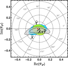
The $68.27\%$ and $95.45\%$ confidence levels for ${\cal R}_{P}$ obtained from the probability distribution functions are shown in Fig. 2 and Fig. 3 for $B\rightarrow\pi\pi$ and $B\to\rho\rho$ decay modes respectively. Also plotted are the corresponding estimates for the observable $S_{00}$, derived from the amplitudes. It can be seen that if $S_{00}$ is measured some of the solutions can be eliminated. In Fig. 2, we have chosen to present only one out of the eight possible solutions where $\tilde{X}+\tilde{Y}$ is in agreement with the SM estimate within one standard deviation. Measurements of the associated time-dependent $C\!P$ asymmetry $S_{00}$ can reduce or even eliminate the ambiguity.

The rotated amplitudes $\tilde{A}^{ij}$ for the decay $B\to\pi\pi$ can also be decomposed [6] in terms of $I=0$ and $I=2$ isospin amplitudes as follows:

with analogous expressions for the three conjugate mode amplitudes $\tilde{\bar{A}}^{ij}$. A graphical representation of Eq. (I) is shown in Fig. 4.

The measurements of the seven observables enable the complete determination of the four isospin amplitudes $\tilde{A}_{0}$, $\tilde{A}_{2}$, $\tilde{\bar{A}}_{0}$ and $\tilde{\bar{A}}_{2}$. The isospin amplitudes $\tilde{A}_{0}$ and $\tilde{A}_{2}$ are easily written in terms of the topological amplitudes as follows:

We have studied the ratios of the isospin amplitudes generically denoted by

Note that $\tilde{A}_{0}/\tilde{A}_{2}=A_{0}/A_{2}$ and $\tilde{\bar{A}}_{0}/\tilde{\bar{A}}_{2}=\bar{A}_{0}/\bar{A}_{2}$.

We find that for $B\to\pi\pi$ the hierarchy of isospin amplitudes is $|A_{2}|\approx|\bar{A}_{2}|\lesssim|A_{0}|<|\bar{A}_{0}|$ whereas for $B\to\rho\rho$ it follows that $|A_{2}|\approx|\bar{A}_{2}|<|A_{0}|\approx|\bar{A}_{0}|$. These observations can be easily verified from Fig. 5 and 6. The right side plot of Fig. 6 deserves special consideration. It is easy to see that $A_{0}/A_{2}$ and $\bar{A}_{0}/\bar{A}_{2}$ can be written in terms of the topological amplitudes and has the form

where $x$, $y$, $\delta_{x}$ and $\delta_{y}$ are complicated function of topological amplitudes and $\alpha$. Hence, the overlapping plots seen the right side figure in Fig. 6 happen if

To conclude we have shown that assuming the value of $\alpha$ obtained from indirect measurements and available experimental data for $B\to\pi\pi$ and $B\to\rho\rho$ observables, all topological and isospin amplitudes can be extracted. These solutions come with an eightfold ambiguity, and only one solution yields small values of electroweak penguins, consistent with SM expectations. Measurements of the associated time-dependent $C\!P$ asymmetry $S_{00}$ can reduce or even eliminate the ambiguity. The interesting conclusion drawn is that the size of that electroweak penguin contributions are consistent with theoretical expectations given the current experimental uncertainties. Improved accuracy in the measurements of observables for these modes and of the indirect measurement of $\alpha$ will help in understanding the electroweak penguin contributions to hadronic modes. We also find a hierarchy among the isospin amplitudes with mild enhancement of the $\Delta I=\tfrac{1}{2}$ transition amplitude.

Acknowledgement: A.K.N. and R.S. would like to thank Sunando Kumar Patra for useful discussions. B.G. thanks Institute of Mathematical Sciences for hospitality where part of the work was done. B.G. was supported in part by the US Department of Energy grant No. de-sc0009919. A.K. thanks SERB India, grant no: SERB/PHY/F181/2018-19/G210, for support. R.S. thanks Perimeter Institute for Theoretical Physics for hospitality where part of this work was done. Research at Perimeter Institute is supported by the Government of Canada through the Department of Innovation, Science and Economic Development and by the Province of Ontario through the Ministry of Research, Innovation and Science.

References

- [1] J. Charles et al. [CKMfitter Group], Eur. Phys. J. C 41, 1 (2005). http://ckmfitter.in2p3.fr
- [2] M. Bona et al. [UTfit Collaboration], JHEP 0610, 081 (2006). http://utfit.org/UTfit/ResultsSummer2018SM.
- [3] D. London and R. D. Peccei, Phys. Lett. B 223, 257 (1989). doi:10.1016/0370-2693(89)90249-9
- [4] B. Grinstein, Phys. Lett. B 229, 280 (1989). doi:10.1016/0370-2693(89)91172-6
- [5] M. Gronau, Phys. Rev. Lett. 63, 1451 (1989). doi:10.1103/PhysRevLett.63.1451
- [6] M. Gronau and D. London, Phys. Rev. Lett. 65, 3381 (1990).
- [7] M. Gronau, O. F. Hernandez, D. London and J. L. Rosner, Phys. Rev. D 52, 6374 (1995) doi:10.1103/PhysRevD.52.6374 [hep-ph/9504327].
- [8] M. Gronau, D. London, N. Sinha and R. Sinha, Phys. Lett. B 514, 315 (2001) doi:10.1016/S0370-2693(01)00818-8 [hep-ph/0105308].
- [9] A. F. Falk, Z. Ligeti, Y. Nir and H. Quinn, Phys. Rev. D 69, 011502 (2004) doi:10.1103/PhysRevD.69.011502 [hep-ph/0310242].
- [10] M. Gronau, D. Pirjol and T. M. Yan, Phys. Rev. D 60, 034021 (1999) Erratum: [Phys. Rev. D 69, 119901 (2004)]
- [11] Y. Amhis et al. [HFLAV Collaboration], arXiv:1812.07461 [hep-ex].
- [12] Y. Amhis et al. [HFLAV Collaboration], Eur. Phys. J. C 77, no. 12, 895 (2017) doi:10.1140/epjc/s10052-017-5058-4 [arXiv:1612.07233 [hep-ex]].
- [13] M. Tanabashi et al. [Particle Data Group], Phys. Rev. D 98, no. 3, 030001 (2018). doi:10.1103/PhysRevD.98.030001.