Constant Power Root Market Makers

We review the marginal price and impermanent loss for the constant sum and product functions, all well known results.

In other words, the price ratio for the constant sum function is fixed. The price is independent of the token reserves. This is not true for the constant product function.

Define the power root value function as

for a fixed constant $p\leq 1$. Note that $p$ does not have to be an integer. Equation 3 is equivalent to a $p$-norm when $a,b,p\geq 0$. However, the two are not identical in properties, particularly in terms of concavity, as we will show in Section 4.2.

We claim that all the value functions corresponding to the constant reserve, sum, and product invariants are special cases of the power root value function. Consider:

Economic Interpretation. We can view value functions as production functions in economic theory. For instance, $V_{\text{prod}}$ is equivalent to the Cobb-Douglas production function, $V_{\text{rsv}}$ is equivalent to the perfect substitute (linear) production function, and $V_{\text{sum}}$ is equivalent to the Leontief production function. Further, $V_{\text{pow}}$ is equivalent to the constant elasticity of substitution, of which the perfect substitute, Leontief, and Cobb-Douglas are special cases of. This matches the result shown in Lemma 4.1.

Before we can apply Equation 2 to derive a trading function, we must verify that $V_{\text{pow}}$ satisfies the four conditions for consistency [1].

Lemma 4.2 shows the power root is a concave function for $p\leq 1$.

As a corollary, we obtain our first theorem.

Now that we have shown $V_{\text{pow}}$ is consistent we are free to compute $\psi_{\text{pow}}=\inf_{a,b\in\mathbf{R}}\{ax+by-V_{\text{pow}}(a,b)\}$ as in Equation 2. We claim the following:

Given the form of Theorem 4.4, we highlight a few special cases. If $p\rightarrow 0$, then $q\rightarrow 0$. If $p\rightarrow-\infty$, then $q\rightarrow 1$. If $p\rightarrow 1$, then $q\rightarrow-\infty$. This is consistent with what we know about constant reserve, sum, and product functions. The value function for the product invariant is also a product, which is shown by $p,q$ both converging to 0 (see Lemma 4.1). The value function for constant sum is a minimum function, which is captured by $q$ converging to 1 when $p$ converges to $-\infty$ (again, recall Lemma 4.1).

Figure 2 visualizes the trading curve for a range of powers $q$. We include $q=0$ (constant product), $q=1$ (constant sum), and $q=-\infty$ (constant reserve, shown in dotted line) for comparisons. We observe that varying $q\in(-\infty,1]$ predictably controls the curvature of the trading function between two extreme functions.

Harmonic Mean Result In the case $q\rightarrow-1$, we recover the constant harmonic mean invariant. By Theorem 4.3, we know $\psi_{\text{har}}(x,y)$ is concave. Further, by Theorem 4.4, we have that its value function is $V_{\text{har}}(a,b)=(a^{\frac{1}{2}}+b^{\frac{1}{2}})^{2}$ as $p=\frac{1}{2}$ when $q=-1$. This function has higher curvature than constant product.

Given the constant power root trading function, we can derive an expression for the marginal price as a function of $p$. The “marginal” price represents the price of one token in terms of the other assuming an infinitesimally small trade.

Begin with $\left((x-\Delta x)^{q}+(y+\Delta y)^{q}\right)^{\frac{1}{q}}=k$. Then $\Delta y=(k^{q}-(x-\Delta x)^{q})^{\frac{1}{q}}-y$. Dividing by $\Delta x$, we obtain $\frac{\Delta y}{\Delta x}=\frac{(k^{q}-(x-\Delta x)^{q})^{\frac{1}{q}}-y}{\Delta x}$. Derive the marginal price using L’Hopital’s rule:

Since $\frac{1}{q}-1=\frac{1-q}{q}$, we obtain the following expression

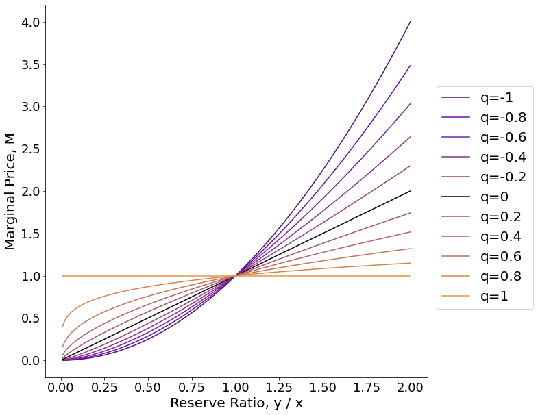
A quick inspection of Equation 4 and Lemma 2.1 shows that for $q=1$, we have $M_{\text{pow}}(1)=x^{0}y^{0}=1=M_{\text{sum}}$, and $M_{\text{pow}}(0)=x^{-1}y^{1}=\frac{y}{x}=M_{\text{prod}}$. That is, the marginal price for the constant sum and product invariants are again, special cases of the constant power root.

Figure 4(a) plots the marginal price as a function of the reserve ratios between $x$ and $y$. As $q\rightarrow 1$, we see the marginal price converge to a constant function at 1. As $q\rightarrow-\infty$, it approaches an exponentially increasing function. When $q=0$, the price is linear.

Using the result in Section 4.3, we show the following theorem:

We plot the impermanent loss as a function of $q$ in Figure 3, where the constant product (i.e. Uniswap) is shown in purple stars, constant reserve is shown in black hexagons, and the constant sum is shown with an orange cross (note this is only a single point as marginal price does not change for the constant sum invariant). Figure 3 shows a gradient of loss functions as $q$ varies. In particular, we see increased impermanent loss as $q$ approaches 1 and reduced impermanent loss as $q$ approaches $-\infty$. This is aligned with prior work [10] that suggests trading functions with flatter curvature have higher loss.

Next, we compute the price impact function [10], or the change to marginal price given a trade of size $\Delta x$, as $\frac{d\Delta y}{d\Delta x}$, the derivative of the price function. Equation 6 shows the price impact function for power roots.

Refer to [10] for derivations for the constant sum and product functions. It is straightforward to show that those are special cases of Equation 6 by $q=0$ and $q=1$. Figure 4(b) shows the price impact for constant power root market makers of varying $q$. When $q\rightarrow 1$, the price impact function approaches 0 slope, which makes sense given that the marginal price is constant when $q=1$. When $q\rightarrow-\infty$, the price impact function has a faster increasing slope, representing higher levels of price sensitivity.

Practically, we note that price impact function is closely related to slippage as a constant function market maker with high price impact will likely experience higher slippage rates. As a base example, when $q=1$, there is zero slippage due to the constant marginal price, or equivalently, its price impact function having zero slope.

In summary, there is a trade-off between impermanent loss and price impact, which is perhaps not surprising. For large negative powers, the invariant has low loss for LPs but high price slippage for traders. For powers close to one, the opposite is true.

Since impermanent loss can be difficult to interpret, we also compute the value $U(x,y,M)$ as well as derivatives with respect to price, such as delta $\Delta=\frac{\delta U}{\delta M}$ and gamma $\Gamma=\frac{\delta^{2}U}{\delta M^{2}}$. Continuing from Section 4.4, we can simplify the expression for value using only the liquidity amount $k$ and the marginal price $M$, removing reserves from the equation:

Taking first and second derivatives, we arrive at closed form expressions for the greeks:

In the following figure, we visualize the greeks for a variety of powers $q$.

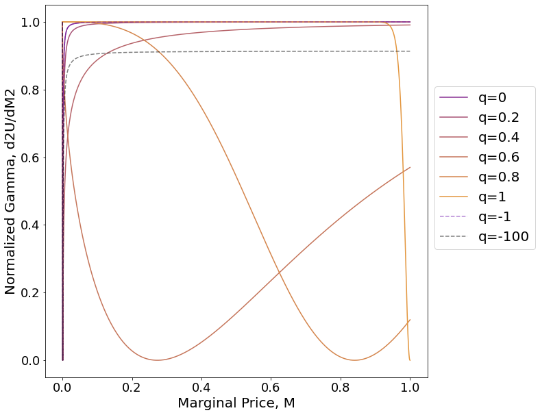
In Figure 5, we vary the marginal price $M$ between 0 and 1 and study the effect on value, delta, and gamma. For each subplot, we normalize the y axis to be between 0 and 1 for visual comparison. As such, the reader should focus on the shape rather than the magnitudes. We make a few observations. First, in Figure 5(a), for positive powers, the larger the power, the less curvature in the value function. Interestingly, for larger negative powers, we observe a similar behavior, as $q=-100$ and $q=1$ have similar shape. Recalling payoff functions from Figure 2, we note that Figure 5(a) shows the same plot in lower dimensions.

Second, we observe more diverse delta functions as $q$ spans between 0 and 1 in Figure 5(b). For smaller positive powers, we observe delta to increase exponentially as price goes to zero, whereas for larger positive powers, we observe delta to increase exponentially as price grows large. For powers close to $q=0.5$, we observe near linear change in delta. Third, in Figure 5(c), we observe that subtle differences in value are exaggerated as gamma functions across powers differ in behavior. This large range in gamma functions may suggest power roots to play a role in structured products to achieve a desired gamma. We note that delta and gamma for negatives powers closely mimic those of constant product.

A benefit of the Uniswap trading function ($q=0$) is a guarantee of no reserve depletion. For any value of token $x>0$ and any constant $k$, we have a $y=\frac{k}{x}>0$. In practice, this implies no trade can conduct a trade large enough to deplete resources. This property, however, does not hold for the sum invariant ($q=1$), where the analogous expression $y=k-x$ suggests that $x\leq k$, otherwise $y\leq 0$.

The power root invariant with $q\leq 0$ guarantees no reserve depletion. However for powers $0<q\leq 1$ it, like the sum, has the same point of reserve depletion, namely $x=k$. One can see this from the equation $y=(k^{q}-x^{q})^{\frac{1}{q}}$, which implies $k^{q}\geq x^{q}$ is required. As $q\rightarrow 0$, this constraint is removed, and power root collapses to product. However, for $q$ closer to 0, we observe more incentives to not deplete reserves due to price increases, though it is theoretically possible. For example, for $q=\epsilon$ close to 0, the marginal price is $\frac{y^{1-\epsilon}}{x^{1-\epsilon}}\approx\frac{y}{x}$. If $x$ is near depleted (and $y$ near $k$), the price will be tending towards $\infty$.

Figure 6 visualizes the relative price between two tokens as a function of trade size in token $x$. Constant sum and product are shown with special markers. We make a few observations. First, the relative price decreases as trade size grows, which is expected given the concavity of the trading functions. Second, for $0<q<1$, the plotted lines intersect the x-axis, representing points of depleted reserves (for $q=1$, we have the point of depletion at $x=1$). For $q\leq 0$, the plotted lines never intersect the x-axis. Third, for $0<q<1$, there are segments where the price is better than constant product, which suggests better conditions for traders assuming small trades. This is not the case for large trades. Clipper [7] formalized this approach by only allowing small trades. For $q<0$, prices are bounded above by constant product ($q=0$), meaning traders face a higher cost.

References

- [1] Guillermo Angeris, Alex Evans, and Tarun Chitra. Replicating market makers. arXiv preprint arXiv:2103.14769, 2021.
- [2] Guillermo Angeris, Hsien-Tang Kao, Rei Chiang, Charlie Noyes, and Tarun Chitra. An analysis of uniswap markets. arXiv preprint arXiv:1911.03380, 2019.
- [3] Hayden Adams, Noah Zinsmeister, Moody Salem, River Keefer, and Dan Robinson. Uniswap v3 core. Technical report, Technical report, 2021.
- [4] Fernando Martinelli and Nikolai Mushegian. A non-custodial portfolio manager, liquidity provider, and price sensor. URl: https://balancer. finance/whitepaper, 2019.
- [5] Alex Evans. Liquidity provider returns in geometric mean markets. arXiv preprint arXiv:2006.08806, 2020.
- [6] Michael Egorov. Stableswap-efficient mechanism for stablecoin liquidity. Retrieved Feb, 24:2021, 2019.
- [7] Abraham Othman. New invariants for automated market making. 2021.
- [8] Allan Niemerg, Dan Robinson, and Lev Livnev. Yieldspace: An automated liquidity provider for fixed yield tokens. 2020.
- [9] Guillermo Angeris and Tarun Chitra. Improved price oracles: Constant function market makers. In Proceedings of the 2nd ACM Conference on Advances in Financial Technologies, pages 80–91, 2020.
- [10] Guillermo Angeris, Alex Evans, and Tarun Chitra. When does the tail wag the dog? curvature and market making. arXiv preprint arXiv:2012.08040, 2020.