Constant Directivity Loudspeaker Beamforming

Beamformer designs for loudspeaker arrays require constraints atypical to their microphone array counterpart due to greater variations in operating frequency characteristics across loudspeaker transducer elements, acoustic and electric power output limits, and placement restrictions. Traditional frequency-invariant beamforming designs for linear [1], circular [2], spherical [3], differential [4, 5] homogeneous arrays often optimize for directivity factor and white-noise gain (WNG) [6], [7], and beam pattern fit [8]. Such constraints are less applicable for heterogeneous loudspeakers and non-uniform arrays that jointly maximize acoustic/electrical power ratio in a listening window, and satisfy a generalized directivity index (GDI) [9]. The former extends WNG to evaluation regions in spherical coordinates, and transducer dependent penalty factors per electrical power unit over frequency. The latter relaxes beam pattern targets to an acoustic power ratio over two evaluation regions defined by density functions. This work addresses both issues and is organized as follows:

Section II introduces a novel regularization technique for the generalized Rayleigh quotient (GRQ) [10] that penalizing both acoustic and electrical power for heterogeneous arrays without introducing explicit constraints in their formulations. Sections II-A, II-B propose two maximal acoustic efficiency and sensitivity beamformer designs subject to constant GDI equality constraints, and present a pair of iterative and analytic solutions respectively via quadratic programming. Section III solves for the secular equation sub-problem common to both beamformer formulations. Section IV shows several beamformer designs for a sample heterogeneous array and compares convergence rates of the iterative solutions. Section V summarizes the theoretical results and experiments.

The GRQ $\frac{\boldsymbol{w}^{H}\boldsymbol{A}\boldsymbol{w}}{\boldsymbol{w}^{H}\boldsymbol{R}\boldsymbol{w}}$ is the power ratio of a beamformer’s responses over two domains specified by weights $\boldsymbol{w}$ and so-called ”accept” and ”reject” covariance matrices $\boldsymbol{A}$, and $\boldsymbol{R}$ respectively. A beamformer’s GDI equates to the GRQ for covariance matrices specified in the acoustic domain given by

where the expectation samples steering vectors or anechoic frequency responses $\boldsymbol{d}(\boldsymbol{r})$ (conjugate transpose $\boldsymbol{d}^{H}(\boldsymbol{r})$) over the Cartesian unit-directions $\boldsymbol{r}$. The probability density functions $f_{A}(\boldsymbol{r})$, $f_{R}(\boldsymbol{r})$ weight the acoustic power-responses over specifiable directions to boost and attenuate respectively as shown in Fig. 1, and generalize the directivity index [9].

Maximizing GRQ therefore maximizes GDI by reducing GRQ into the normal Rayleigh quotient under a change of variables:

where matrix $\boldsymbol{L}$ is the lower-triangular Cholesky factor of $\boldsymbol{R}$. The maximizer $\boldsymbol{w}_{*}=\operatorname*{arg\,max}_{\boldsymbol{w}}G(\boldsymbol{A},\boldsymbol{R},\boldsymbol{w})=\boldsymbol{L}^{-H}\boldsymbol{v}$ of (2) constrained to the unit-circle $\boldsymbol{w}^{H}\boldsymbol{R}\boldsymbol{w}=1$ is therefore the eigenvector $\boldsymbol{v}$ of the largest eigenvalue of matrix $\boldsymbol{Q}$.

In heterogeneous transducer beamformer design, it is beneficial to mix both acoustic and electric rejection covariance matrices as to penalize components of $\boldsymbol{w}$ outside each transducer’s operating frequency ranges. Consider the following generalized Rayleigh penalty quotient (GRPQ) $G(\boldsymbol{A},\boldsymbol{R}+\boldsymbol{\Gamma}\boldsymbol{\Sigma},\boldsymbol{w})$ which adds a diagonal positive-definite penalty matrix $\boldsymbol{\Gamma}\boldsymbol{\Sigma}$ to the denominator covariance matrix $\boldsymbol{R}$ given by

where $0\leq\sigma_{n}\leq\infty$ is unbounded. Inverting the sum of $\boldsymbol{\Sigma}$ and the identity matrix $\boldsymbol{I}$ gives the bounded weighting matrix

which penalizes $\left|{w_{n}}\right|$ for smaller $\lambda_{n}$. Lowering $\lambda_{n}\rightarrow 0$ for frequencies outside transducer $n$’s operating range has the desired effect on the maximizer $\left|{w_{n*}}\right|\rightarrow 0$ and thus generalizes crossover designs to joint frequency-transducer weighted specifications of $\boldsymbol{\Lambda}$ as shown in Fig. 2.

For computation, $\boldsymbol{\Lambda}$ also improves the condition number of $\boldsymbol{\Gamma}\boldsymbol{\Sigma}$ for maximizing (2) when combined with the following change of variables:

where $\boldsymbol{y}=\boldsymbol{\Lambda}^{-1}\boldsymbol{w}$. The modified GRPQ in (5) is now well-conditioned and bounded above by GRQ as expressed by

where $\boldsymbol{\hat{R}}$ attenuates non-diagonal entries of $\boldsymbol{R}$ by $\boldsymbol{\Lambda}^{2}$.

The secular equations $S(\lambda)$ in (15), (23) can be expressed in rational form w.r.t. reciprocal eigenvalue poles $b_{n}=e_{n}^{-1}$:

where $u_{n}$ and $e_{n}$ are the $n$th elements of $\boldsymbol{u}$ and $\textbf{{diag}}\left[{\boldsymbol{E}}\right]$ from (15), (23) respectively, and $a_{n}=\left|{u_{n}}\right|^{2}$. It is also useful to express $S(\lambda)=S_{\raisebox{0.0pt}{\scalebox{0.85}{-}}}(\lambda)+S_{\raisebox{0.0pt}{\scalebox{0.55}{+}}}(\lambda)$ and its first derivative in terms of the set of negative and positive poles $B_{\raisebox{0.0pt}{\scalebox{0.85}{-}}}=\left\{{b_{n}|\,b_{n}<0}\right\}$ and $B_{\raisebox{0.0pt}{\scalebox{0.55}{+}}}=\left\{{b_{n}|\,b_{n}>0}\right\}$ respectively given by

Unlike the linear and quadratic secular equations in [13], $S(\lambda)$ is not monotonic in most intervals between consecutive poles due to the presence of different signed $b_{n}$ in the numerator terms. The one exception is the tightest interval bounding $0$ which contains the smallest magnitude negative and positive poles $b_{\raisebox{0.0pt}{\scalebox{0.85}{-}}}=\max\left({B_{\raisebox{0.0pt}{\scalebox{0.85}{-}}}}\right)$, $b_{\raisebox{0.0pt}{\scalebox{0.55}{+}}}=\min\left({B_{\raisebox{0.0pt}{\scalebox{0.55}{+}}}}\right)$ respectively. This is a consequence of (25) where the first derivatives given by

in the intervals outside these poles are bounded and positive.

Moreover, we show as in Fig. 3 that the intersecting interval $b_{\raisebox{0.0pt}{\scalebox{0.85}{-}}}<\lambda<b_{\raisebox{0.0pt}{\scalebox{0.55}{+}}}$ contains exactly one real-valued root $\lambda_{*}$ that is also the root nearest to $0$ and therefore equivalent to the critical point and solutions to (12), (20). The proof is as follows:

The function $S(b_{\raisebox{0.0pt}{\scalebox{0.85}{-}}}<\lambda<b_{\raisebox{0.0pt}{\scalebox{0.55}{+}}})$ where $S(\lambda=b_{\raisebox{0.0pt}{\scalebox{0.85}{-}}})=-\infty$, $S(\lambda=b_{\raisebox{0.0pt}{\scalebox{0.55}{+}}})=+\infty$ is continuous and so the intermediate value theorem guarantees the existence of at least one real-valued root in the interval. Its first derivative $\frac{\partial\,{S(b_{\raisebox{0.0pt}{\scalebox{0.85}{-}}}<\lambda<b_{\raisebox{0.0pt}{\scalebox{0.55}{+}}})}}{\partial\,{\lambda}}>0$ is strictly positive in the interval via (26) and therefore contains exactly one root $\lambda_{*}$ that can easily be found via bracketing methods such as [19]. To show that $\lambda_{*}$ is indeed the nearest to $0$, observe that reflecting $\lambda$ over $b_{\raisebox{0.0pt}{\scalebox{0.85}{-}}}$ or $b_{\raisebox{0.0pt}{\scalebox{0.55}{+}}}$ in the interval moves $\lambda$ closer to the remaining poles in $B_{-}$, $B_{+}$ respectively:

which with (26) places bounds on $S_{\raisebox{0.0pt}{\scalebox{0.85}{-}}}(\lambda)$, $S_{\raisebox{0.0pt}{\scalebox{0.55}{+}}}(\lambda)$ given by

and as a result induces bounds on $S(\lambda)$ after summation:

This implies there are no roots in the regions reflected across $b_{\raisebox{0.0pt}{\scalebox{0.85}{-}}}$ and $b_{\raisebox{0.0pt}{\scalebox{0.55}{+}}}$ given by $2b_{\raisebox{0.0pt}{\scalebox{0.85}{-}}}-\lambda_{*}<\lambda<b_{\raisebox{0.0pt}{\scalebox{0.85}{-}}}$ and $b_{\raisebox{0.0pt}{\scalebox{0.55}{+}}}<\lambda<2b_{\raisebox{0.0pt}{\scalebox{0.55}{+}}}-\lambda_{*}$ respectively and that $\lambda_{*}$ must be nearest to $0$.

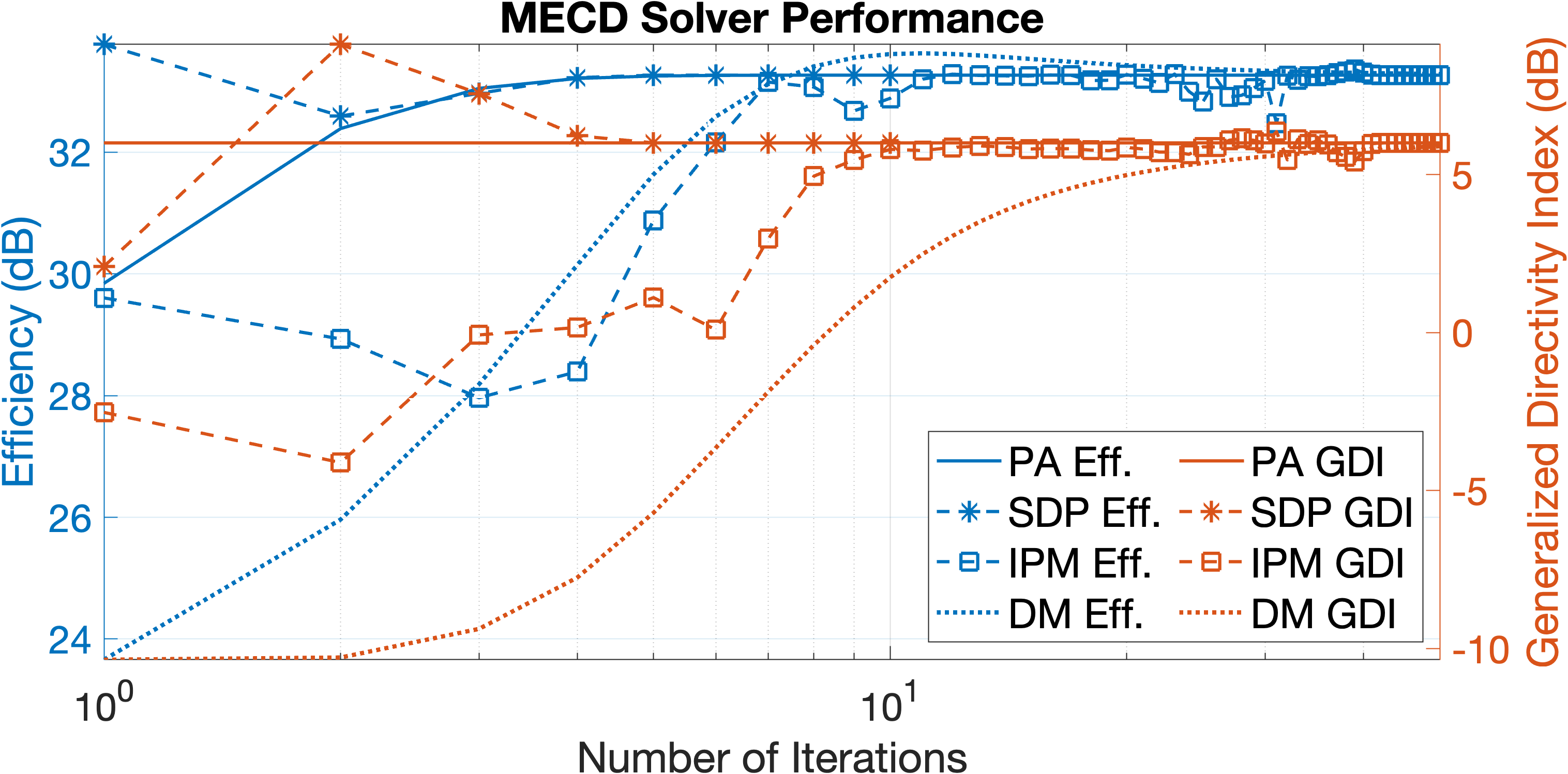
We first compare MECD solver performance for $N=8$ elements with randomized complex-valued covariances $\boldsymbol{A},\boldsymbol{R},\boldsymbol{C}$ in Fig. 4. Our PA method reduces the number of iterations to convergence of the baseline DM method from $50$ to $5$. Larger step-sizes in the latter cause oscillations between the objective and constraint, and also exhibit to a lesser degree in Matlab’s fmincon IPM solver. SDPT3 [20] for SDP shows similar convergence rates of the objective to PA but requires more compute in solving for $N^{2}$ number of variables instead of $N$.

We then compare GRQ to GRPQ beamformer designs for a measured sample $N=3$ mid-range, full-range, and tweeter array with $\boldsymbol{A},\boldsymbol{R},\boldsymbol{C}=\boldsymbol{A}$ integrated over densities from Fig. 1, frequency weighting $\Lambda$ from Fig. 2, and constant GDI $\min\left\{{6,\,10\log_{10}\max(\tau)}\right\}\textrm{ dB}$ for MECD and MSCD. GRPQ beam patterns shown in Fig. 5 exhibit more regular responses inline with expected transducer operating frequency ranges; directivity grows increasingly omni-directional in low-frequency as only the mid-range is active. MECD beam patterns exhibit less lobing than MSCD and their maximum GDI counterparts.

We introduced an electrical power penalty term to GRQ for regularizing frequency-dependent heterogeneous speaker array beamformer designs such as MECD and MSCD. Characterizing the projection sub-problem in MECD-PA and MSCD yielded a fast quadratic secular equation root-finding solution. The PA method accelerated convergence rates over the baseline DM, IPM, and SDP methods. GRPQ solutions exhibited more regular beam patterns than GRQ for a sample $3$-way system. Inequality constrained GDI can be considered in future works.

The necessary conditions for $(\boldsymbol{v},\lambda)$ in (12) are given by

where several useful relations are derived for characterizing the minimizer. Expanding the equality constraint in (30) relates the sum of symmetric terms to the sum of mixed terms:

It is possible to relate the squared norm of $\boldsymbol{v}$ from (30) to the difference in squared norms under $\boldsymbol{D}$ via (31):

For $(\boldsymbol{v}_{1},\lambda_{1})$, $(\boldsymbol{v}_{2},\lambda_{2})$, the mixed products from (30) are given:

where their arithmetic mean is equivalent under conjugation $\boldsymbol{v}_{2}^{H}\boldsymbol{v}_{1}=\frac{1}{2}\left({\boldsymbol{v}_{2}^{H}\boldsymbol{v}_{1}+\left({\boldsymbol{v}_{1}^{H}\boldsymbol{v}_{2}}\right)^{H}}\right)$ and $\boldsymbol{v}_{1}^{H}\boldsymbol{v}_{2}=\left({\boldsymbol{v}_{2}^{H}\boldsymbol{v}_{1}}\right)^{H}$:

Summing (34) and substituting (31) gives

Subtracting (35) from the sum of $(\boldsymbol{v}_{1},\lambda_{1})$, $(\boldsymbol{v}_{2},\lambda_{2})$ substituted into (32) gives $\boldsymbol{v}_{1}^{H}\boldsymbol{v}_{1}+\boldsymbol{v}_{2}^{H}\boldsymbol{v}_{2}-\boldsymbol{v}_{2}^{H}\boldsymbol{v}_{1}-\boldsymbol{v}_{1}^{H}\boldsymbol{v}_{2}=\left({\boldsymbol{v}_{1}-\boldsymbol{v}_{2}}\right)^{H}\left({\boldsymbol{v}_{1}-\boldsymbol{v}_{2}}\right)$ which verifies (17). Next, observe that the arithmetic difference is equivalent under conjugation:

whereby taking the summation and substituting (31) gives

Subtracting (37) from the difference $\boldsymbol{v}_{1}^{H}\boldsymbol{v}_{1}-\boldsymbol{v}_{2}^{H}\boldsymbol{v}_{2}$ after substitution into (32) verifies (16) after combining the terms.

References

• [1] D. B. Ward, R. A. Kennedy, and R. C. Williamson, Constant directivity beamforming.   Springer, 2001, pp. 3–17.
• [2] G. Huang, J. Chen, and J. Benesty, “Insights into frequency-invariant beamforming with concentric circular microphone arrays,” IEEE/ACM Trans. Audio, Speech, Language Process., vol. 26, no. 12, 2018.
• [3] F. Zotter, H. Pomberger, and A. Schmeder, “Efficient directivity pattern control for spherical loudspeaker arrays,” Journal of the Acoustical Society of America, vol. 123, no. 5, p. 3643, 2008.
• [4] J. Wang, W. Zhang, C. Pan, J. Chen, and J. Benesty, “On the design of differential loudspeaker arrays with broadside radiation patterns,” JASA Express Letters, vol. 1, no. 8, 2021.
• [5] F. Miotello, A. Bernardini, D. Albertini, F. Antonacci, and A. Sarti, “Steerable first-order differential loudspeaker arrays with monopole and dipole elements,” in Convention of the European Acoustics Association, Forum Acusticum, 2023, pp. 11–15.
• [6] R. Berkun, I. Cohen, and J. Benesty, “Combined beamformers for robust broadband regularized superdirective beamforming,” IEEE/ACM Trans. Audio, Speech, Language Process., vol. 23, no. 5, 2015.
• [7] M. Crocco and A. Trucco, “Design of robust superdirective arrays with a tunable tradeoff between directivity and frequency-invariance,” IEEE Trans. Signal Process., vol. 59, no. 5, 2011.
• [8] L. C. Parra, “Steerable frequency-invariant beamforming for arbitrary arrays,” The Journal of the Acoustical Society of America, vol. 119, no. 6, pp. 3839–3847, 2006.
• [9] Y. Luo, “Spherical harmonic covariance and magnitude function encodings for beamformer design,” EURASIP Journal on Audio, Speech, and Music Processing, vol. 2021, pp. 1–17, 2021.
• [10] R. Horn and C. Johnson, Matrix Analysis.   Cambridge University Press, 1990.
• [11] J. Platt and A. Barr, “Constrained differential optimization,” in Neural Information Processing Systems, D. Anderson, Ed., vol. 0.   American Institute of Physics, 1987.
• [12] W. Gander, “Least squares with a quadratic constraint,” Numerische Mathematik, vol. 36, pp. 291–307, 1980.
• [13] G. H. Golub, “Some modified matrix eigenvalue problems,” SIAM Review, vol. 15, no. 2, p. 330, 1973.
• [14] A. Shapiro, “Rank-reducibility of a symmetric matrix and sampling theory of minimum trace factor analysis,” Psychometrika, vol. 47, pp. 187–199, 1982.
• [15] A. I. Barvinok, “Problems of distance geometry and convex properties of quadratic maps,” Discrete & Computational Geometry, vol. 13, pp. 189–202, 1995.
• [16] G. Pataki, “On the rank of extreme matrices in semidefinite programs and the multiplicity of optimal eigenvalues,” Mathematics of Operations Research, vol. 23, 05 1998.
• [17] D. Davis, E. Patronis, and P. Brown, Sound System Engineering 4e.   Taylor & Francis, 2013, pp. 365–366.
• [18] W. Gander, G. H. Golub, and U. Von Matt, “A constrained eigenvalue problem,” Linear Algebra and its applications, vol. 114, pp. 815–839, 1989.
• [19] R. P. Brent, “An algorithm with guaranteed convergence for finding a zero of a function,” The Computer Journal, vol. 14, no. 4, 1971.
• [20] K.-C. Toh, M. J. Todd, and R. H. Tütüncü, “SDPT3 — a matlab software package for semidefinite programming, version 1.3,” Optimization methods and software, vol. 11, no. 1-4, pp. 545–581, 1999.