Consistent Spectral Clustering in Hyperbolic Spaces
Abstract
Clustering, as an unsupervised technique, plays a pivotal role in various data analysis applications. Among clustering algorithms, Spectral Clustering on Euclidean Spaces has been extensively studied. However, with the rapid evolution of data complexity, Euclidean Space is proving to be inefficient for representing and learning algorithms. Although Deep Neural Networks on hyperbolic spaces have gained recent traction, clustering algorithms or non-deep machine learning models on non-Euclidean Spaces remain underexplored. In this paper, we propose a spectral clustering algorithm on Hyperbolic Spaces to address this gap. Hyperbolic Spaces offer advantages in representing complex data structures like hierarchical and tree-like structures, which cannot be embedded efficiently in Euclidean Spaces. Our proposed algorithm replaces the Euclidean Similarity Matrix with an appropriate Hyperbolic Similarity Matrix, demonstrating improved efficiency compared to clustering in Euclidean Spaces. Our contributions include the development of the spectral clustering algorithm on Hyperbolic Spaces and the proof of its weak consistency. We show that our algorithm converges at least as fast as Spectral Clustering on Euclidean Spaces. To illustrate the efficacy of our approach, we present experimental results on the Wisconsin Breast Cancer Dataset, highlighting the superior performance of Hyperbolic Spectral Clustering over its Euclidean counterpart. This work opens up avenues for utilizing non-Euclidean Spaces in clustering algorithms, offering new perspectives for handling complex data structures and improving clustering efficiency.
Keywords— Hyperbolic Space, Spectral Clustering, Hierarchical Structure, Consistency
1 Introduction
In the realm of machine learning, the pivotal process of categorizing data points into cohesive groups remains vital for uncovering patterns, extracting insights, and facilitating various applications such as customer segmentation, anomaly detection, and image understanding [1]. Among the paradigms of clustering algorithms [2], alongside Partitional, Hierarchical, and Density-based techniques, Spectral Clustering on Euclidean spaces has garnered extensive research attention [3]. Spectral clustering operates in the spectral domain, utilizing the eigenvalues and eigenvectors of the Laplacian of a similarity graph constructed from the data. This algorithm initially constructs a similarity graph, where nodes represent data points and edges indicate pairwise similarities or affinities among the data points. It then computes the graph Laplacian matrix, capturing the graph’s structural properties and encoding relationships among the data points. Since its inception [See [4] and [5]], the Euclidean version of Spectral Clustering has significantly evolved. For simple clustering with two labels, this method considers the eigenvector corresponding to the second smallest eigenvalue of a specific graph Laplacian constructed from the affinity matrix based on the spatial position of the sample data. It then performs the -means clustering on the rows of the Eigenmatrix [whose columns consist of the eigenvectors corresponding to the smallest two eigenvalues], treating the rows as sample data points, and finally returns the cluster labels to the original dataset. This particular form of spectral clustering finds applications [6] in Speech Separation [7], Image Segmentation [8], Text Mining [9], VLSI design [10], and more. A comprehensive tutorial is also available at [3]. Here, we will briefly review the most commonly used Euclidean Spectral Clustering Algorithm.
When connectedness is a crucial criterion for the clustering algorithms, the conventional form of Spectral Clustering emerges as a highly effective approach. It transforms the standard data clustering problem in a given Euclidean space into a graph partitioning problem by representing each data point as a node in the graph. Subsequently, it determines the dataset labels by discerning the spectrum of the graph. Beginning with a set of data points . A symmetric similarity function (also known as the kernel function) , along with the number of clusters , we construct the similarity matrix . In its simplest form, Spectral Clustering treats the similarity matrix as a graph and aims to bipartite the graph to minimize the sum of weights across the edges of the two partitions. Mathematically, we try to solve an optimization problem [3] of the following form:
| (1.1) |
where is the Graph Laplacian and the degree matrix and . is a label feature matrix, being the number of label features. Then, the simplest form of spectral clustering aims to minimize the trace by the feature matrix by considering the first eigenvectors of as its rows.
In order to extend the algorithm to form clusters, we consider the eigenvectors corresponding to the smallest eigenvalues of . Then, treating the rows of the Eigenmatrix as sample data points in , we perform the means clustering and label them. Finally, we return the labels to the original data points in the order they were taken to construct the degree matrix . Some of the variants of this algorithm can be found at [3].


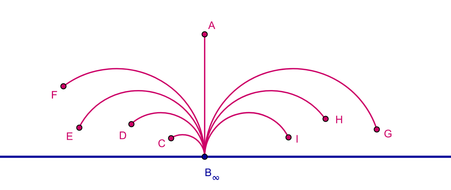
This form of Euclidean Spectral Clustering works well on Euclidean datasets, which are relatively simple and have some distinct connectedness. But as data evolves rapidly and takes extremely complex shapes, Euclidean space becomes a more inefficient model space in capturing the intricate patterns in the data and thereby helping learning algorithms in that set-up. Thus, visualizing data from a more complex topological perspective and developing unsupervised learning techniques on these complex shapes can have a consequential impact on revealing the true nature of the data. Although Deep Neural Networks on hyperbolic spaces have recently gained some attention and found applications in various computer vision problems [see [11], [12], [13], [14]], clustering algorithms or non-deep machine learning models on non-Euclidean Spaces are one of the least explored domains. In this paper, we scrutinize this domain by proposing a spectral clustering algorithm on hyperbolic spaces. While Euclidean Space fails to provide meaningful information and lacks its representational power in implementing arbitrary tree/graph-like structures or hierarchical data, that can not be embedded in Euclidean Spaces with arbitrary low dimensions, and at the same time, these spaces do not preserve the associated metric (similarity measure/dissimilarity measure), hyperbolic spaces can be beneficial to implement the structure obtained from these examples [see [15], [16]] and even some hyperbolic spaces with shallow dimension can be very powerful to represent these data and clustering on these spaces can result in far better efficiency compared to the clustering in Euclidean Spaces like Figure 1. Our main contributions to this paper are:
-
•
We propose the spectral clustering algorithm on hyperbolic spaces in which an appropriate hyperbolic similarity matrix replaces the Euclidean similarity matrix.
-
•
We also provide a theoretical analysis concerning the weak consistency of the algorithm and prove that it converges (in the sense of distribution) at least as fast as the spectral clustering on Euclidean spaces.
- •
Having said that, we organize the rest of our paper in the following way. In Section 2, we will give a brief overview of the works related to the Euclidean Spectral Clustering and its variants. We will also discuss why we need to consider a hyperbolic version of the Euclidean Spectral Clustering and some of its variants. Section 3 lays out the mathematical backgrounds pertaining to our proposed algorithm. We will discuss several results which will enable us to formulate the algorithm in a rigorous manner. We give the details of our proposed algorithm in Section 4. We discuss the motivation behind the steps related to our algorithm. Section 5 has been dedicated for the proof of the weak consistency of the proposed algorithm. Section 6 presents and discusses the experimental results. Finally, conclusions are drawn in Section 7.
2 Related Works
We commence with a brief overview of prominent variants of Euclidean spectral clustering:
-
1.
Bipartite Spectral Clustering on Graphs (ESCG): Introduced by Liu et al. [17] in 2013, this algorithm primarily aims to reduce the time complexity during spectral decomposition of the affinity matrix by appropriately transforming the input similarity matrix of a Graph dataset. The method involves randomly selecting seeds from a given Graph of input size , followed by generating supernodes using Dijkstra’s Algorithm to find the shortest distance from the Graph nodes to the seeds. This process reduces the size of the similarity matrix , where is the indicator matrix of size and is the original affinity matrix. Subsequently, it proceeds with spectral decomposition of the normalized , where and are diagonal matrices containing the column and row sums of , respectively. The algorithm computes the largest eigenvectors of and generates clusters based on the -means algorithm on the matrix , where is the right singular matrix in the singular value decomposition of .
-
2.
Fast Spectral Clustering with approximate eigenvectors (FastESC): Developed by He et al. [18] in 2019, this algorithm initially performs -means clustering on the dataset with a number of clusters greater than the true clusters and then conducts spectral clustering on the centroids obtained from the -means. Similar to ESCG, this algorithm also focuses on reducing the size of the input similarity matrix for spectral clustering.
-
3.
Low Rank Representation Clustering (LRR): Assuming a lower-rank representation of the dataset , where each is the -th data vector in , this algorithm aims to solve an optimization problem to minimize the rank of a matrix subject to . Here, is a dictionary, and is the coefficient matrix representing in a lower-dimensional subspace. The algorithm iteratively updates and an error matrix as proposed by Liu et al. in [19].
Among other variants of Spectral Clustering, such as Ultra-Scalable Spectral Clustering Algorithm (U-SPEC) [20] or Constrained Laplacian Rank Clustering (CLR) [21], the primary objective remains consistent - to enhance efficiency by reducing the burden of the spectral decomposition step through minimizing the size of the input similarity matrix. However, there has been minimal exploration regarding the translation of these algorithms into a hyperbolic setup. In this context, this marks the initial attempt to elevate non-deep machine learning algorithms beyond Euclidean Spaces.
Consider a dataset with a hierarchical structure, represented as a top-to-bottom tree. As we traverse along nodes away from the root, the distance among nodes at the same depth but with different parents grows exponentially with respect to their heights. This exponential growth renders Euclidean Space unsuitable as a model space for representing the hierarchy. Hyperbolic spaces are better suited for this purpose, where distance grows exponentially as we move away from the origin/root node. Some of these issues have been addressed in a series of papers [11], [12], [14] in the context of Deep Neural Networks. Recently in context to downstream self-supervised tasks, the authors in [22] presented scalable Hyperbolic Hierarchical Clustering (sHHC), which learns continuous hierarchies in hyperbolic space. Leveraging these hierarchies from sound and vision data, hierarchical pseudo-labels are constructed, leading to competitive performance in activity recognition compared to recent self-supervised learning models. In this work, we propose a general-purpose spectral clustering algorithm on a chosen hyperbolic space after embedding the original Euclidean dataset into the space in a particular way that minimally perturbs the inherent hierarchy.
3 Mathematical Preliminaries
3.1 Smooth Manifold
Manifolds:
A topological space is locally Euclidean of dimension n, if for every , there exists a neighbourhood and a map such that , being open in , is a homeomorphism. We call such a pair () a chart or co-ordinate system on . An dimensional Topological Manifold is a Hausdorff, Second Countable and Locally Euclidean of dimension [see [24]].
Charts and Atlas:
We say two charts and to be compatible if and only if and are maps between Euclidean Spaces. A Atlas or simply an Atlas on a Euclidean Space is a collection such that ’s are pairwise compatible and . It is worth noting that any Atlas is Contained in a unique Maximal Atlas.
Smooth Manifold:
A smooth or manifold is a topological manifold equipped with a maximal atlas. Throughout this article, we will exclusively refer to a smooth manifold when discussing manifolds.
Consider a point . If two functions coincide on certain neighborhoods around , their directional derivatives will also be identical. This allows us to establish an equivalence relation among all functions within some neighborhood of . Let be a neighborhood of , and consider all where is . We define two functions and as equivalent if there exists a neighborhood such that when restricted to . This equivalence relation holds for all functions at , forming what is known as the set of germs of functions on at , denoted as . Similarly, this notion extends to manifolds through charts, where represents the germs of all functions on at .
Derivation and Tangent Space:
A Derivation on is a linear map:
satisfying the Libneiz’s Rule:
A tangent vector at is a Derivation at . The vector space of all tangent vectors at is denoted as .
Let be a chart around . Let . Let be the standard coordinates on . Then . If , then . If , .
Vector Fields:
A Vector Field on an open subset of is a function that assigns to each point to a tangent vector in . Since form a local basis of , .
Cotangent Space and Differential Forms:
Let us also talk briefly about the dual of Tangent Space, also known as the Cotangent Space. It consists of the space of all covectors or linear functionals on the Tangent Space and is denoted by . Similarly, here we can define Covector Fields or Differential 1-Form on an open set of that assigns to each point , a covector . Staying consistent with the notation, forms a local basis of Cotangent Space dual to , i.e.
where when and is otherwise.
Tensor Product:
If is a -linear function and is a -linear function on a vector space , their tensor product is defined to be the linear function as
where are arbitrary vectors in .
3.2 Riemannian Manifold
Riemannian Manifolds:
A Riemannian Manifold is a smooth manifold equipped with a smooth Riemannian Metric [23], i.e. a map , i.e. , , i.e. is a bilinear functional on . [] If is a chart on , taking and ,
Now we state an elementary result from the Riemannian Geometry without proof.
Proposition 3.1:
Every smooth manifold admits a Riemannian Metric.
Corollary 1:
The Usual Spectral Clustering Algorithm on Euclidean Spaces can be applied to Riemannian Manifolds with the Euclidean Metric replaced by Riemannian Metric, at least locally. In particular it can be applied to compact subsets of model hyperbolic spaces with the corresponding hyperbolic metric.
Length and Distance:
Let be a piecewise smooth curve. The length of , is defined as, . Given two points , we define the distance between and as: such that is a peicewise smooth curve and . This distance is also known as the Geodesic Distance between and on .
Proposition 3.2:
Let be a Riemannian Manifold with Riemannian metric . Then is a metric space with the distance function defined as above. The metric topology on coincides with the manifold topology.
Let denote the space of all vector fields on . Let . Then . . Considering only second component of a vector field, . Hence . Given , we define the covariant derivative of in the direction of by . For , is defined as . This defines a map as
-
(i)
and .
-
(ii)
and .
-
(iii)
and .
This is called an induced connection on and it satisfies two properties:
-
1.
(Symmetry) .
-
2.
(Metric Compatibility) .
This on is called the Levi-Civita Connection or the Riemannian Connection. It can be proved that there exists a unique such connection on a given Riemannian Manifold satisfying symmetry and metric compatibility.
Curvature Operator:
The curvature operator on is defined as the -trilinear map:
as
.
Sectional Curvature:
Let and be a two dimensional subspace. The curvature of in the direction of is defined as
| (3.1) |
where
| (3.2) |
Hyperbolic Spaces:
An -dimensional hyperbolic space is characterized as the singularly connected, -dimensional complete Riemannian Manifold with a constant sectional curvature of . Represented as , it stands as the exclusive simply connected -dimensional complete Riemannian Manifold with a constant negative sectional curvature of . The renowned Killing-Hopf Theorem [26] affirms that any two such Riemannian Manifolds are isometrically equivalent. While numerous isometric model spaces exist, we will only touch upon four of them briefly. The geodesics on these spaces are illustrated in Figure 2.
-
1.
Poincaré Half Space Model: This is the upper half plane . The metric on this space is defined as follows: suppose and are two points whose distance we want to compute. Let be the reflection of with respect to the plane . Then
(3.3) (3.4) -
2.
Poincaré Disc Model: This is a model hyperbolic space in which all points are inside the unit ball in and geodesics are either diameters or circular arcs perpendicular to the unit sphere. The metric between two points and ()is defined as
-
3.
Beltrami-Klein Model: This is a model hyperbolic space in which points are represented by the points in the open unit disc in and lines are represented by chords, special type of straight lines with ideal end points on the unit sphere. For , the open unit ball, the distance in this model is given as
(3.5) where are ideal points on the boundary sphere of the line with and .
-
4.
Hyperboloid Model: This is a model hyperbolic space also known as Minkowski Model which is the forward sheet of the two hyperbolic sheets embedded in the dimensional Minkowski Space. The hyperbolic distance between two points and is given as
(3.6) where
Note that is simply the Minkowski Dot Product.
Gyrovector Space:
The concept of Gyrovector Space, introduced by Abraham A. Ungar [see [27]], serves as a framework for studying vector space structures within Hyperbolic Space. This abstraction allows for the definition of special addition and scalar multiplications based on weakly associative gyrogroups. For a detailed geometric formalism of these operations, Vermeer’s work [28] provides an in-depth exploration.
In this context, we will briefly discuss Mbius Gyrovector Addition and Mobius Scalar Multiplication on the Poincar’e Disc. Due to isometric transformations between hyperbolic spaces of different dimensions, the same additive and multiplicative structures can be obtained for other model hyperbolic spaces [see [29]]. Utilizing Mbius addition and multiplication is essential when evaluating intrinsic metrics like the Davies-Bouldin Score or Calinski-Harabasz Index to assess the performance of our proposed algorithm.
-
1.
Mbius Addition: For two points and in the Poincaré Disc, the Mbius addition is defined as: where is the curvature and for hyperbolic spaces, .
-
2.
Mbius Scalar Multiplication: For , and in the Poincaré Disc, the scalar multiplication is defined as: This addition and scalar multiplication satisfy the axioms pertaining to the Gyrovector Group [see [27]].


4 Proposed Algorithm
Before discussing the proposed spectral clustering algorithm, we will briefly talk about an equivalent formulation of the Euclidean Spectral Clustering algorithm. In the Introduction LABEL:sec:introduction section, we described the spectral clustering problem as trace minimization problem. In its simplest form, if the two clusters are and , then solving 1.1 is equivalent to minimize the normalized cut (N-Cut) problem
| (4.1) |
where and . But 4.1 is an NP-hard problem in general. To ease this problem, we tend to solve another equivalent minimization problem
| (4.2) |
Here we choose such that
In order to solve 4.2 we construct the Normalized Graph Laplacians as
or
and then converting 4.2 to
| (4.3) |
where is either or . Then solving the generalized eigenvalue problem of the form of 4.2 is transformed into an eigenvalue problem of the form . Since the smallest eigenvalue of is , the Rayleigh Quotient 4.3 is minimized at the eigenvector corresponding to the next smallest eigenvalue. More generally, if the number of clusters is , we have to choose the eigenvectors corresponding to the smallest eigenvalues.
Having all these preliminaries and the equivalent formulations, we are now ready to discuss our proposed algorithm. At first, we need to identify carefully the appropriate model space on which we will consider our data points. Since the hyperbolic space of dimension is not bounded, if we consider data points spreading across the entire space, we might run into problems to verify its consistency. To remove this shortcoming, we will consider only a compact subset of our model space chosen carefully.
Since the boundary of the model hyperbolic space is at infinite distance from the origin (for example, the plane in Poincaré half space model or the unit circle in Poincaré disc model), we have to consider only a compact subset of in order to talk about general notion of convergence. More specifically, we will fix some and consider the following subsets of for either Poincaré half space model or disc model:
-
•
Poincaré Half Space Model: Consider .
-
•
Poincaré Disc Model: Consider .
Note that if we choose sufficiently small, then the clusters will not be affected by the choice of . Since the formation of clusters depends only on the spatial position of the data points among themselves, choosing a bigger only affect in terms of scaling. However, in order to utilize the hyperbolic nature of we will choose to be very small, let’s say in the order of .
Since every dimensional model hyperbolic space is isometric to each other by the Killing-Hopf Theorem, for the purpose of convergence, it is reasonable to talk about a compact subset of only one of the model hyperbolic spaces. For our purpose, we will only consider the above mentioned compact subset of the Poincaré Disc Model and denote it by , more explicitly, equipped with the Poincaré metric

4.1 The Hyperbolic Spectral Clustering Algorithm (HSCA)
Let for some . We will follow the graph-based clustering methods where the edge of a graph (in the Euclidean Space) will be replaced by corresponding Geodesics in . Below we elaborate on the steps of HSCA. For clarity, a pseudo-code of the algorithm is provided in Algorithm 1.
-
1.
Embed the original dataset into the Poincaré Disc of unit radius. Obtain such that , where can be taken any small number, let’s say , like Figure 3.
-
2.
Construct the graph where . The edge set where is the geodesic from to on .
-
3.
For the each geodesic-edge (from now on we will use edge instead of geodesic-edge) attach a weight which measures the similarity between the respective nodes and . The set of weights define the proximity matrix or affinity matrix, this is the matrix such that
The proximity matrix is symmetric. A common choice of the proximity matrix is the Gaussian Kernel or the Poisson Kernel(the same Gaussian kernel or Poisson Kernel on Euclidean Space with the metric replaced by geodesic distance on ). can be represented as
for the Gaussian Kernel, or
for the Poisson Kernel, where is pre-defined cut-off distance set by the user.
-
4.
Now treat as the new data matrix, i.e. treat each row (or column since is symmetric) of as new data lying in , call each row of by , where each is a representative of the original data . Compute the modified affinity matrix .
-
5.
Next compute the degree matrix , where . Construct the graph Laplacian . Next construct the normalized graph Laplacian .
-
6.
Compute the first eigenvectors of the normalized graph Laplacian corresponding to the first eigenvalues of of . Call this matrix . Normalize the rows of , construct such that
-
7.
For , let be the th row of .
-
8.
Form clusters from the points using means algorithm. The clusters are .
4.1.1 Explanation:
Step 1 is clear, since our model space is a subset of the Poincaré Disc, we have to embed each data point into the space. While doing that we have taken each point and divided it by it’s Euclidean norm plus some small positive integer. This will ensure that the data points in the similar hierarchy will be closed in the embedding. Next we have computed the affinity matrix by treating each edge between points as geodesic edge and have the Poincaré metric absorbed into the corresponding Kernel. Next we have constructed the modified similarity matrix mainly by keeping the idea that if the points and in the embedded dataset are closed to a set of same points, then they should ideally belong to the same cluster. The spectral decomposition modified similarity matrix will ensure that the representative points in the rows of will form the cluster closed to the ground level. Rest of the steps are taken from the well known normalized Euclidean Spectral Clustering Algorithm proposed by Ng, Jordan and Weiss [30].
Input: Dataset , number of clusters=, hyperparameter , cut-off length=.
Output: Cluster labels where .
Time Complexity:
The most computationally intense step is to perform the spectral decomposition of the similarity matrix which takes time [31]. Calculating the pairwise Poincare Distance and the similarity matrix each takes time. Finally applying the means during the eigenvalue decomposition takes amount of time, where is the number of data points, is the number of clusters, is the number of means iterates and is the dimension of the Hyperbolic Space .
4.2 Approximated Hyperbolic Spectral Clustering with Poincaré -Means Based landmark Selection (HLS K)
Here we shortly describe another variant of the HSCA proposed with an analogy to the Approximated Spectral Clustering with -Means based landmark Selection, one variant of the ESCA. We assume the form of the input dataset as . We also assume the number of landmark points are , where has to be chosen carefully such that , where is the number of original clusters and also should not be very small compared to . [For example, if the number of samples is , and , we can choose or .] The steps of the algorithm are provided as follows: [For details we refer to the supplementary]
-
1.
We obtain such that , where small, let’s say .
-
2.
Next we perform the initial Poincaré Means [This is a Means clustering with the Euclidean Distance replaced by the Poincar’e Distance] to form clusters, namely with centroids of these clusters as respectively.
-
3.
Now we construct such that or .
-
4.
Then we normalize the columns of , i.e., form the matrix with . Construct the diagonal matrix with . Construct . Form the final matrix .
-
5.
Finally we follow steps of HSCA (Algorithm 1) to form the clusters.
5 Verifying The Consistency of HSCA
Following our previous notations, and are two points on the Poincaré Disc and the metric is given as
where
The Hyperbolic Gaussian Kernel is given as
and the Hyperbolic Poisson Kernel is given as
At first, we will prove the consistency of the HSCA using Gaussian Kernel. The proof will be quite similar if we use the Poisson Kernel. Before that we will look at a couple of results involved in the consistency proof.
Lemma 5.1.
For the usual Euclidean Gaussian Kernel given by , we have whenever .
Proof.
See Appendix A. ∎
Remark 5.1.
Remark 5.2.
is radial: If we fix one variable, let’s say at , then , which is a radial function. Therefore, the Poincaré Metric is also radial, so is the Hyperbolic Gaussian Kernel.
Lemma 5.2.
The hyperbolic Gaussian Kernel , i.e. this kernel is an absolutely integrable.
Proof.
See Appendix A. ∎
Terminology:
For a compact subset [with in its interior], we call to be symmetric if for every and for every , we have .
Lemma 5.3.
Suppose is symmetric, and is radial. Then its Fourier Transform is also radial.
Proof.
See Appendix A. ∎
Next we intend to use Theorem 3 [32] and this necessitates computing the Fourier Transform of and will show that decays exponentially.
Lemma 5.4.
There exist such that for all .
Proof.
See Appendix A. ∎
Terminology and Definitions:
Let be the compact subset of the Poincaré Disc as defined above. be the similarity function with the Gaussian Kernel equipped with the Poincaré Metric. Let be the normalized similarity function. Then for any continuous function , we define the following [as in section 6 [33]:
We also define . Now we will re-write Theorem 19[33] with a slightly modified proof.
Theorem 5.1.
Let be a probability space with being any arbitrary sigma algebra on . Let be defined as above with . Let be a sequence of i.i.d. random variables drawn according to the distribution and be the corresponding emperical diustributions. Then there exists a constant such that for all with probability at least ,
where is the covering number of the space with ball of radius with respect to the metric . Hence the rate of convergence of the Hyperbolic Spectral Clustering is .
Proof.
See Appendix A. ∎
Remark 5.3.
Note that in deriving the convergence rate of the hyperbolic spectral clustering, we used results used mostly in the proof of the consistency of spectral clustering in the Euclidean set-up. The hyperbolic metric is in general very powerful compared to the squared euclidean metric, which forces the hyperbolic Gaussian/Poisson Kernel converging to much faster than the Euclidean ones. Therefore, we believe the convergence rate of the hyperbolic spectral clustering can be improved, which requires estimating a careful bound on the logarithmic covering number with respect to the hyperbolic metric.
6 Experiments and Results
6.1 Description of the Datasets:
To examine the clustering efficiency of our proposed algorithm, we will use a combination of total datasets, among these are real datasets Airport, Glass, Zoo and Wisconsin and are synthetic datasets 2d-20c-no0, D31, and st900. The ground cluster levels are not available in case of the Airport dataset. Details of the datasets are shown in Table 1. Since the Airport dataset is too large, we took random samples of sizes , , and four times to evaluate the clustering efficiency assuming the number of ground clusters being .
| Datasets | No. of Samples | Dimension | Number of Clusters |
|---|---|---|---|
| Airport | 1048575 | 196 | - |
| Wisconsin | 699 | 9 | 2 |
| Glass | 214 | 9 | 6 |
| Zoo | 101 | 16 | 7 |
| 2d-20c-no0 | 1517 | 2 | 20 |
| st900 | 900 | 2 | 9 |
| D31 | 3100 | 2 | 31 |
| Methods | Airport(1000) | Airport(2000) | ||||
|---|---|---|---|---|---|---|
| S. Score | D.B. Score | C.H. Index | S. Score | D.B. Score | C.H. Index | |
| ESCA(G) | 0.68 | 0.75 | 78.62 | 0.83 | 0.12 | 189.66 |
| HSCA(G) | 0.24 | 0.31 | 1114.77 | 0.21 | 0.32 | 2023.64 |
| Improvement | 64.7% () | 44%() | 1317.9%() | 74.7%() | 166.7%() | 967.0%() |
| ESCA(P) | 0.70 | 0.40 | 140.02 | 0.82 | 0.40 | 93.31 |
| HSCA(P) | 0.21 | 0.32 | 1111.89 | 0.17 | 0.34 | 2024.71 |
| Improvement | 70.0% () | 20%() | 694.1%() | 79.27%() | 17.7%() | 2069.87%() |
| Methods | Airport(5000) | Airport(10000) | ||||
| S. Score | D.B. Score | C.H. Index | S. Score | D.B. Score | C.H. Index | |
| ESCA(G) | 0.57 | 0.56 | 144.84 | 0.83 | 0.46 | 218.53 |
| HSCA(G) | 0.24 | 0.32 | 5299.59 | 0.24 | 0.33 | 10584.5 |
| Improvement | 57.9% () | 42.9%() | 3558.9%() | 71.1%() | 28.3%() | 4755.1%() |
| ESCA(P) | 0.57 | 0.56 | 144.83 | 0.83 | 0.26 | 218.53 |
| HSCA(P) | 0.21 | 0.34 | 5258.51 | 0.21 | 0.35 | 10428.3 |
| Improvement | 63.2% () | 39.3%() | 3531.1%() | 74.7%() | 34.6%() | 4672.1%() |
| Methods | Wisconsin Breast Cancer | Glass | ||||
| S. Score | D.B. Score | C.H. Index | S. Score | D.B. Score | C.H. Index | |
| ESCA(G) | 0.41 | 0.49 | 3.44 | 0.53 | 0.28 | 9.94 |
| HSCA(G) | 0.01 | 0.91 | 131.54 | 0.42 | 0.10 | 111.66 |
| Improvement | 97.56% () | 85.7%() | 3723.8%() | 20.8%() | 64.3%() | 1023.3%() |
| ESCA(P) | 0.46 | 0.40 | 5.12 | 0.57 | 0.26 | 10.56 |
| HSCA(P) | 0.27 | 0.65 | 219.06 | 0.28 | 0.12 | 110.72 |
| Improvement | 41.3% () | 62.5%() | 4280.1%() | 50.1%() | 53.8%() | 948.5%() |
| Methods | Zoo | 2d-20c-no0 | ||||
| S. Score | D.B. Score | C.H. Index | S. Score | D.B. Score | C.H. Index | |
| ESCA(G) | 0.22 | 0.64 | 13.51 | 0.54 | 0.64 | 1953.87 |
| HSCA(G) | 0.32 | 0.16 | 49.62 | 0.47 | 0.16 | 9630.12 |
| Improvement | 45.5% () | 75.0%() | 267.3%() | 12.9%() | 75.0%() | 393.9%() |
| ESCA(P) | 0.23 | 0.96 | 5.94 | 0.35 | 0.71 | 2.27 |
| HSCA(P) | 0.35 | 0.17 | 50.85 | 0.54 | 0.10 | 8643.90 |
| Improvement | 52.2% () | 82.3%() | 756.1%() | 54.3%() | 85.9%() | %() |
| Methods | st900 | D31 | ||||
| S. Score | D.B. Score | C.H. Index | S. Score | D.B. Score | C.H. Index | |
| ESCA(G) | -0.03 | 0.68 | 75.31 | 0.39 | 0.56 | 2365.22 |
| HSCA(G) | 0.47 | 0.86 | 1548.80 | 0.17 | 0.85 | 2102.17 |
| Improvement | 1667.7% () | 26.5%() | 1956.6%() | 56.4%() | 51.8%() | 11.12%() |
| ESCA(P) | -0.03 | 0.67 | 75.28 | 0.17 | 0.95 | 185.07 |
| HSCA(P) | 0.49 | 0.63 | 2388.67 | 0.50 | 0.57 | 69144.07 |
| Improvement | 1733.3% () | 6.0%() | 3073.1%() | 194.1%() | 40.0%() | 37261%() |
6.2 Performance Measure and Validity Index:
When the true cluster labels of the datasets are not known, we will use three intrinsic cluster performance measures to compare the Euclidean Spectral Clustering algorithm with the Hyperbolic Spectral Clustering Algorithm. We will use three main intrinsic evaluation metrics, namely
Also, for simulated datasets, we know the true cluster labels and the number of clusters. There we will compare ESCA and HSCA by the extrinsic evaluation metrics, namely


| Methods | Wisconsin | Glass | Zoo | 2d-20c-no0 | st900 | D31 | ||||||
|---|---|---|---|---|---|---|---|---|---|---|---|---|
| ARI | NMI | ARI | NMI | ARI | NMI | ARI | NMI | ARI | NMI | ARI | NMI | |
| ESCA(G) | 0.01 | 0.01 | 0.01 | 0.06 | 0.26 | 0.37 | 0.67 | 0.86 | 0.16 | 0.35 | 0.56 | 0.84 |
| HSCA(G) | 0.77 | 0.66 | 0.23 | 0.36 | 0.53 | 0.70 | 0.76 | 0.87 | 0.72 | 0.76 | 0.22 | 0.60 |
| Improvement | 7600% () | 6500%() | 2200%() | 500%() | 104%() | 89%() | 13%() | 1.1%() | 350%() | 117%() | 60%() | 29%() |
| ESCA(P) | 0.01 | 0.01 | 0.01 | 0.05 | 0.14 | 0.34 | 0.12 | 0.42 | 0.17 | 0.35 | 0.09 | 0.45 |
| HSCA(P) | 0.16 | 0.24 | 0.25 | 0.38 | 0.57 | 0.76 | 0.60 | 0.82 | 0.63 | 0.71 | 0.29 | 0.63 |
| Improvement | 1500%() | 2300%() | 2400%() | 660%() | 307%() | 124%() | 400%() | 95%() | 354%() | 103%() | 222%() | 40%() |
| ELSC-K(G) | 0.82 | 0.72 | 0.23 | 0.40 | 0.70 | 0.78 | 0.54 | 0.79 | 0.72 | 0.78 | 0.94 | 0.96 |
| HLSC-K(G) | 0.84 | 0.73 | 0.25 | 0.39 | 0.71 | 0.78 | 0.55 | 0.80 | 0.75 | 0.81 | 0.95 | 0.97 |
| Improvement | 2.4%() | 1.4%() | 8.7%() | 2.5%() | 1.4%() | 0.00%(-) | 1.9%() | 1.3%() | 4.2%() | 3.8%() | 1%() | 1%() |
| ELSC-K(P) | 0.86 | 0.76 | 0.25 | 0.39 | 0.49 | 0.70 | 0.54 | 0.79 | 0.72 | 0.80 | 0.95 | 0.96 |
| HLSC-K(P) | 0.87 | 0.78 | 0.27 | 0.41 | 0.79 | 0.77 | 0.53 | 0.78 | 0.69 | 0.73 | 0.96 | 0.98 |
| Improvement | 1.1%() | 2.6%() | 8%() | 2.5%() | 5.1%() | 10%() | 1.9%() | 1.3%() | 4.2%() | 8.75%() | 1%() | 1%() |
| FESC(G) | 0.01 | 0.01 | 0.01 | 0.07 | 0.12 | 0.23 | 0.25 | 0.73 | 0.11 | 0.21 | 0.02 | 0.28 |
| FHSC(G) | 0.05 | 0.02 | 0.02 | 0.04 | 0.36 | 0.52 | 0.13 | 0.39 | 0.24 | 0.48 | 0.14 | 0.67 |
| Improvement | 400%() | 100%() | 100%() | 43% () | 200%() | 126%() | 48%() | 47%() | 118%() | 129%() | 600%() | 139%() |
| FESC(P) | 0.01 | 0.01 | 0.03 | 0.07 | 0.11 | 0.24 | 0.16 | 0.44 | 0.11 | 0.22 | 0.10 | 0.38 |
| FHSC(P) | 0.84 | 0.75 | 0.25 | 0.37 | 0.68 | 0.77 | 0.37 | 0.79 | 0.70 | 0.78 | 0.94 | 0.96 |
| Improvement | 8300%() | 7400%() | 733%() | 429% () | 518%() | 221%() | 131%() | 79%() | 536%() | 254%() | 840%() | 153%() |
| LRR | -0.01 | 0.00 | -0.03 | 0.12 | 0.01 | 0.07 | -0.00 | 0.04 | 0.00 | 0.04 | 0.00 | 0.03 |
6.3 Effectiveness of HSCA:
We now assess the performance of our proposed HSCA against the following well-known versions of the Spectral Clustering algorithms [with the Gaussian (G) and Poisson (P) kernels]:
-
1.
Euclidean Spectral Clustering Algorithm [ESCA] [3]
-
2.
Fast Euclidean Spectral Clustering Algorithm [18] [we have also developed a hyperbolic version of FESC, which we named as Fast Hyperbolic Spectral Clustering Algorithms (FHSC) analogously to the HSCA and included in our comparison]
-
3.
Low Rank Representation Clustering (LRR) [19]
-
4.
Approximated spectral clustering with -means-based landmark selection (ELSC-K) [39] [we have also compared it with the respective hyperbolic variants HLSC-K with respect to the Gaussian(G) and Poisson Kernels(P)]. See Supplementary for a pseudo-code of the algorithm.
6.4 Discussions:
When analyzing the outcomes presented in Tables 2 and 3, let’s delve into the alterations in the evaluation metrics resulting from running the variants of the HSCA as specified. In Table 2, we’ve outlined the outcomes from executing the variants of ESCA alongside their corresponding hyperbolic versions. We will handle the Airport dataset separately since there are no ground cluster levels available for it. Furthermore, the Airport dataset is categorical, inheriting a hierarchical structure. When a dataset includes a hierarchy, the initial transformation of HSCA embeds the dataset closer to a similar hierarchy compared to other points appearing in different hierarchies. Consequently, the hyperbolic distance between points in similar hierarchies becomes significantly smaller compared to distances between points in different hierarchies, where Euclidean Spaces exhibit poor performance. Once the embedding process is complete, the remainder of HSCA categorizes the points almost according to their hierarchy.
6.4.1 Airport Dataset:
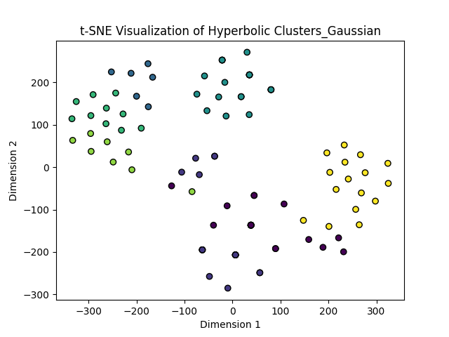
If we compare the obtained numerical results with the visual clusters depicted through the t-SNE plot in Fig. 6, we observe that for the Airport dataset, the Silhoutte Score have been significantly decreased in the HSCA compared to the ESCA. This is primarily due to the fact that both the ESCA(G) and ESCA(P) have given one predominant clusters, whereas the HSCA clusters have given distinct clusters. Since the Silhoutte Score increases if the mean distance between clusters in the same dataset decreases and the mean smallest distance from the other clusters increases, the ESCA clusters are expected to give higher Silhoutte Score compared to the HSCA clusters simply because there are more distinct clusters formed in HSCA. On the other hand, the Davies-Bouldin score depends on the distances between the centroids of the same cluster vs the distances between cluster centroids in distinct clusters. Unlike the Silhoutte Score, there is a drastic change between the values in the Davies-Bouldin Scores compared to the Euclidean with respect to the Hyperbolic, formation of more distinct clusters along with the incorporated the hyperbolic metric to compute the particluar score have resulted in the drastic change. A good cluster is generally charecterized by the higher Silhoutte Score (closer to 1), lower Davies-Bouldin Score (preferably lower than 1) but high Calinski-Harabasz Score. Aparently HSCA performs poorly compared to the ESCA if the first two metrics are considered, but the Calinski-Harabasz Indices have gone significantly high in the case of HSCA, this is again due to incorporating the hyperbolic metric and the nature of distribution that the index follows. Since the ground level clusters are not available for this dataset and it has some inherent hierarchical structure, we can conclude the HSCA has surmounted the ESCA by giving more distinct clusters.
Upon scrutinizing the numerical outcomes alongside the visual representations of clusters portrayed in the t-SNE plot in Fig. 6, a notable trend emerges within the Airport dataset: the Silhouette Score experiences a significant decline in the HSCA compared to the ESCA. This phenomenon can be attributed to the fact that both the ESCA(G) and ESCA(P) methods yield one predominant cluster, whereas the HSCA approach generates five distinct clusters. Given that the Silhouette Score is contingent upon a reduction in the mean distance between clusters within the same dataset and an increase in the mean smallest distance from other clusters, it follows that ESCA clusters are predisposed to higher Silhouette Scores relative to HSCA clusters due to the greater number of distinct clusters formed by HSCA. Conversely, the Davies-Bouldin score hinges on the distances between centroids within the same cluster versus the distances between cluster centroids in distinct clusters. In contrast to the Silhouette Score, there is a notable disparity in the Davies-Bouldin Scores between the Euclidean and Hyperbolic scenarios, resulting from the formation of more distinct clusters and the incorporation of the hyperbolic metric in computing the score. A desirable cluster is typically characterized by a higher Silhouette Score (closer to 1), a lower Davies-Bouldin Score (preferably below 1), and a high Calinski-Harabasz Score. Although HSCA appears to underperform compared to ESCA based on the first two metrics, the Calinski-Harabasz Indices show a significant increase in the case of HSCA. This improvement is once again attributed to the incorporation of the hyperbolic metric and the distribution nature that the index follows. Despite the unavailability of ground-level clusters for this dataset and its inherent hierarchical structure, we can infer that HSCA outperforms ESCA by yielding more distinct clusters.
6.4.2 Other Real Datasets: Wisconsin, Glass & Zoo
Here we examine the effects of HSCA versus ESCA for the Wisconsin Breast Cancer, Glass, and Zoo datasets. In all these three cases, HSCA variants outperform ESCA clusters [see 6 and the supplementary document]. This is primarily attributed to the datasets possessing some form of hierarchical structure. When embedding them into Euclidean Spaces, poor cluster formations arise. Notably, only the Approximated Spectral Clustering with -means based landmark selection (ELSC-K) exhibits superior performance compared to standard Euclidean Spectral Clustering. This can be attributed to the -means based landmark selection, which captures the inherent hierarchy to some extent, leading to improved spectral clusterings. However, Hyperbolic variants of ELSC-K still outperform, as the hyperbolic space is better suited for embedding hierarchical data.
6.4.3 Synthetic Datasets: 2d-20c-no0, st900 & D15
The similar clustering forms also work for these datasets. The Poincaré embedding takes care of the part that the points in the same hierarchy will remain close. Here we also observe that the variants of HSCA perform way better than the corresponding variants of the ESCA as expected. The ESCA and HSCA clusters formed on the st-900 dataset have been shown in Figure 6. For other synthetic datasets, we refer to the supplementary.
6.5 Ablation Experiments
The kernel hyperparameter requires tuning to achieve optimal performance. In our experiments, we set to a small value (approximately ), which has been found to be optimal for most variants of the HSCA. We have observed that there is minimal fluctuation in the ARi or NMi values when the hyperparameter values ( for the Gaussian Kernel and for the Poisson Kernel) are very small (less than ). These values exhibit bounded variation within a small range when the hyperparameter is very small. Our approach for this analysis follows a similar methodology to that presented in [40]. For detailed graphs illustrating the tuning process, please refer to Figures 7 and 8.
The clusters related to other datasets can be found in Section Experiments and Results of the supplementary document.


7 Conclusion
In this paper, we highlight the limitations of Euclidean space in conveying meaningful information and representing arbitrary tree or graph-like structures. We emphasize the inability of Euclidean spaces with low dimensions to embed such structures while preserving the associated metric. Conversely, Hyperbolic Spaces offer a compelling solution, even in shallow dimensions, to efficiently represent such data and yield superior clustering results compared to Euclidean Spaces. Our primary contributions include proposing a spectral clustering algorithm tailored for hyperbolic spaces, where a hyperbolic similarity matrix replaces the traditional Euclidean one. Additionally, we provide theoretical analysis on the weak consistency of the algorithm, showing convergence at least as fast as spectral clustering on Euclidean spaces. We also introduce hyperbolic versions of well-known Euclidean spectral clustering variants, such as Fast Spectral Clustering with approximate eigenvectors (FastESC) and Approximate Spectral Clustering with -means-based Landmark Selection.
Our approach to clustering data in hyperbolic space via spectral decomposition of the modified similarity matrix reveals a more effective method for clustering complex hierarchical data compared to Euclidean Spaces. Notably, this algorithm converges at least as rapidly as Spectral Clustering on Euclidean Spaces without introducing additional computational complexity. Moreover, variants of Hyperbolic Spectral Clustering exhibit superior adequacy and performance over their Euclidean counterparts. We anticipate that this method will expedite significant advancements in non-deep machine learning algorithms.
Availability of Datasets and Codes:
The airport dataset is available on https://www.kaggle.com/datasets/tylerx/flights-and-airports-data. The other real datasets have been taken from https://github.com/milaan9/Clustering-Datasets/tree/master/01.%20UCI and the synthetic datasets are available https://github.com/milaan9/Clustering-Datasets/tree/master/02.%20Synthetic.
References
- [1] A. E. Ezugwu, A. M. Ikotun, O. O. Oyelade, L. Abualigah, J. O. Agushaka, C. I. Eke, A. A. Akinyelu, A comprehensive survey of clustering algorithms: State-of-the-art machine learning applications, taxonomy, challenges, and future research prospects, Engineering Applications of Artificial Intelligence, Vol. 110, 2022.
- [2] M. Filippino, F. Camastra, F. Masulli, S. Rovetta, A survey of kernel and spectral methods for clustering, Pattern Recognition, Volume 41, Issue 1, January 2008, Pages 176-190 https://doi.org/10.1016/j.patcog.2007.05.018.
- [3] U. Luxburg, A Tutorial on Spectral Clustering, Statistics and Computing, 17 (4), 2007 https://doi.org/10.1007/s11222-007-9033-z.
- [4] W. E. Donath and A. J. Hoffman, Lower Bounds for the Partitioning of Graphs, IBM Journal of Research and Development, vol. 17, no. 5, pp. 420-425, Sept. 1973, https://doi.org/10.1147/rd.175.0420.
- [5] M. Fiedler, Algebraic connectivity of graphs, Czechoslovak Mathematical Journal, 23.2 (1973): 298-305 http://eudml.org/doc/12723
- [6] S.V. Suryanarayana, G.V. Rao, G. V. Swamy, A Survey : Spectral Clustering Applications and its Enhancements, International Journal of Computer Science and Information Technologies, Vol. 6 (1) , 2015, 185-189 https://ijcsit.com/docs/Volume%206/vol6issue01/ijcsit2015060141.pdf
- [7] F. R. Bach, M. I. Jordan, Learning Spectral Clustering, With Application To Speech Separation, Journal of Machine Learning Research 7 (2006) 1963-2001 https://jmlr.csail.mit.edu/papers/volume7/bach06b/bach06b.pdf
- [8] F. Tung, A. Wong, D. A. Clausi, Enabling scalable spectral clustering for image segmentation, Pattern Recognition, 43 (2010), 4069-4076 https://uwaterloo.ca/vision-image-processing-lab/sites/ca.vision-image-processing-lab/files/uploads/files/enabling_scalable_spectral_clustering_for_image_segmentation_1.pdf
- [9] I. Dhillon, Co-clustering documents and words using bipartite spectral graph partitioning, Proceedings of the Seventh ACM SIGKDD International Conference on Knowledge Discovery and Data Mining (KDD) 269–274. ACM Press, New York (2001) https://www.cs.utexas.edu/users/inderjit/public_papers/kdd_bipartite.pdf
- [10] L. Hagen and A. B. Kahng, New spectral methods for ratio cut partitioning and clustering, IEEE Transactions on Computer-Aided Design of Integrated Circuits and Systems, vol. 11, no. 9, pp. 1074-1085, Sept. 1992 https://doi.org/10.1109/43.159993
- [11] W. Peng, T. Varanka, A. Mostafa, H. Shi and G. Zhao, Hyperbolic Deep Neural Networks: A Survey in IEEE Transactions on Pattern Analysis & Machine Intelligence, vol. 44, no. 12, pp. 10023-10044, 2022 https://doi.ieeecomputersociety.org/10.1109/TPAMI.2021.3136921.
- [12] O. E. Ganea, G. Bécigneul, T. Hofmann, Hyperbolic Neural Networks,32nd Conference on Neural Information Processing Systems (NeurIPS 2018), Montréal, Canada https://proceedings.neurips.cc/paper_files/paper/2018/file/dbab2adc8f9d078009ee3fa810bea142-Paper.pdf
- [13] W. Chen, X. Han, Y. Lin, H. Zhao, Z. Liu, P. Li, M. Sun, J. Zhou, Fully Hyperbolic Neural Networks, Proceedings of the 60th Annual Meeting of the Association for Computational Linguistics Volume 1: Long Papers, pages 5672 - 5686, May 22-27, 2022 https://aclanthology.org/2022.acl-long.389.pdf
- [14] I. Chami, R. Ying, C. Ré, J. Leskovec, Hyperbolic Graph Convolutional Neural Networks, Advances in Neural Networks Processing Systems, 2019 Dec; 32: 4869–4880 https://pubmed.ncbi.nlm.nih.gov/32256024/.
- [15] N. Lu, H. Miao, Clustering Tree-Structured Data on Manifold, IEEE Transactions on Pattern Analysis & Machine Intelligence, VOL. 38, NO. 10, October 2016 https://ieeexplore.ieee.org/document/7346489.
- [16] Mondal, R., Ignatova, E., Walke, D. et al. Clustering graph data: the roadmap to spectral techniques, Discov Artif Intell 4, 7 (2024) https://link.springer.com/article/10.1007/s44163-024-00102-x.
- [17] J. Liu, C. Wang, M. Danilevsky, and J. Han, “Large-scale spectral clustering on graphs,” Proceedings on 23rd International Joint Conference on Artificial Intelligence, 2013, pp. 1486–1492 https://dl.acm.org/doi/abs/10.5555/2540128.2540342.
- [18] L. He, N. Ray, Y. Guan, H. Zhang, Fast Large-Scale Spectral Clustering via Explicit Feature Mapping, IEEE Transactions on Cybernetics, vol. 49, no. 3, pp. 1058-1071, March 2019 https://ieeexplore.ieee.org/document/8281623.
- [19] G. Liu, Z. Lin, Y. Yong, Robust subspace segmentation by low-rank representation, Proceedings of the 27th International Conference on Machine Learning, 2010, pp. 663–670 https://people.eecs.berkeley.edu/~yima/matrix-rank/Files/lrr.pdf.
- [20] D. Huang, C. Wang, J. Wu, J. Lai, and C. Kwoh, Ultra-scalable spectral clustering and ensemble clustering, IEEE Transaction on Knowledge and Data Engineering, vol. 32, no. 6, pp. 1212–1226, Jun. 2020 https://ieeexplore.ieee.org/stamp/stamp.jsp?arnumber=8661522.
- [21] F. Nie, X. Wang, M. I. Jordan, H. Huang, The Constrained Laplacian Rank Algorithm for Graph-Based Clustering, Proceedings of the Thirtieth AAAI Conference on Artificial Intelligence (AAAI-2016) https://dl.acm.org/doi/abs/10.5555/3016100.3016174.
- [22] T. Long, N. Noord, Cross-modal Scalable Hyperbolic Hierarchical Clustering, 2023 IEEE/CVF International Conference on Computer Vision (ICCV), Pages: 16609-16618.
- [23] M. P. do Carmo, Riemannian Geometry, Birkhuser Boston, MA https://link.springer.com/book/9780817634902
- [24] L. W. Tu, Differential Geometry: Connections, Curvature, and Characteristic Classes, Springer International Publishing https://www.google.co.in/books/edition/Differential_Geometry/bmsmDwAAQBAJ?hl=en.
- [25] S. Lang, Differential and Riemannian Manifolds, Springer New York, https://www.google.co.in/books/edition/Differential_and_Riemannian_Manifolds/K-QlBQAAQBAJ?hl=en.
- [26] J. M. Lee, Riemannian Manifolds: An Introduction to Curvature, Springer New York https://www.google.co.in/books/edition/Riemannian_Manifolds/92PgBwAAQBAJ?hl=en.
- [27] A. A. Ungar, A Gyrovector Space Approach to Hyperbolic Geometry, Morgan and Claypool Publishers https://www.google.co.in/books/edition/A_Gyrovector_Space_Approach_to_Hyperboli/dlFTgrhqm3IC?hl=en&gbpv=0.
- [28] J. Vermeer, A geometric interpretation of Ungar’s addition and of gyration in the hyperbolic plane, Topology and its Applications 152 (2005) 226–242 https://core.ac.uk/download/pdf/82435867.pdf.
- [29] J. G. Ratcliffe, Foundations of Hyperbolic Manifolds, Springer International Publishing https://www.google.co.in/books/edition/Foundations_of_Hyperbolic_Manifolds/yMO4DwAAQBAJ?hl=en&gbpv=0
- [30] A. Ng, M. Jordan, Y. Weiss, On Spectral Clustering: Analysis and an algorithm, Advances in Neural Information Processing Systems, vol 14 (2001), https://proceedings.neurips.cc/paper_files/paper/2001/file/801272ee79cfde7fa5960571fee36b9b-Paper.pdf.
- [31] S. Tsioronis, M. Sozio, M. Vazirgiannis, Accurate Spectral Clustering for Community Detection in MapReduce, (2013), https://api.semanticscholar.org/CorpusID:16810309.
- [32] D. Zhou, The Covering Number in Learning Theory, JOURNAL OF COMPLEXITY, vol. 18, 739–767 (2002) https://doi.org/10.1006/jcom.2002.0635.
- [33] U. Luxburg, M. Belkin, O. Bousquet, Consistency of spectral clustering, Annals of Statistics. 36(2): 555-586 (April 2008) https://doi.org/10.1214/009053607000000640.
- [34] K. R. Shahapure, C. Nicholas, Cluster Quality Analysis Using Silhouette Score, IEEE 7th International Conference on Data Science and Advanced Analytics (DSAA), Sydney, NSW, Australia, 2020, pp. 747-748 https://ieeexplore.ieee.org/document/9260048.
- [35] J. C. R. Thomas, M. S. Peas, M. Mora, New Version of Davies-Bouldin Index for Clustering Validation Based on Cylindrical Distance, 2013 32nd International Conference of the Chilean Computer Science Society (SCCC), Temuco, Chile, 2013, pp. 49-53 https://ieeexplore.ieee.org/document/7814434.
- [36] S. Łukasik, P. A. Kowalski, M. Charytanowicz, P. Kulczycki, Clustering using flower pollination algorithm and Calinski-Harabasz index, 2016 IEEE Congress on Evolutionary Computation (CEC), Vancouver, BC, Canada, 2016, pp. 2724-2728 https://ieeexplore.ieee.org/document/7744132
- [37] M. J. Warrens, H. van der Hoef, Understanding the Adjusted Rand Index and Other Partition Comparison Indices Based on Counting Object Pairs, Journal of Classification, 39, 487–509 (2022). https://link.springer.com/article/10.1007/s00357-022-09413-z#citeas.
- [38] P. A. Estevez, M. Tesmer, C. A. Perez, J. M. Zurada, Normalized Mutual Information Feature Selection, IEEE Transactions on Neural Networks, vol. 20, no. 2, pp. 189-201, Feb. 2009 https://ieeexplore.ieee.org/document/4749258.
- [39] X. Chen, D. Cai, Large Scale Spectral Clustering with Landmark-Based Representation, Proceedings of the Twenty-Fifth AAAI Conference on Artificial Intelligence https://xinleic.xyz/papers/aaai11.pdf
- [40] L. Bai, J. Liang, Y. Zhao, Self-Constrained Spectral Clustering , IEEE Transactions on Pattern Analysis and Machine Intelligence, vol. 45, no. 4, pp. 5126-5138, 1 April 2023 https://ieeexplore.ieee.org/document/9813560
8 Appendix
9 Proofs of Lemmas and Theorem from Section 5
9.1 Proof of Lemma 5.1
Proof.
Step 1: We have , hence . Hence we can write
But we also have
Combining this with the last inequality, we get
Step 2: For , . Therefore the inverse sine hyperbolic function is a strictly increasing function of . By Step 1, we have . Therefore, we have . This also implies .
Since and the inverse sine hyperbolic function is increasing, we can write
We know that for , . This enables us to write
Step 3: Note that for , . Let . Then is differentiable and we get . Therefore is increasing on and for , . Hence . Therefore following step 2, we get
∎
9.2 Proof of Lemma 5.2
9.3 Proof of Lemma 5.3
Proof.
is radial if and only if for every [where is the special unitary group on , i.e. consisting of all matrices over with determinant ], [as the operation only rotates , does not change its magnitude, i.e. ]. Then for any arbitrary
where the second equality follows from the fact that we get by the conjugate linearity of the inner product: since []. ∎
9.4 Proof of Lemma 5.4
Proof.
Let . Then by Lemma 5.1, we have for all . Exploiting fully the fact that is radial (and hence real valued), we get
where and are some appropriately chosen constants. ∎
9.5 Proof of Theorem 5.1
Proof.
Combining Lemma 5.4 and Theorem 3 [32] we get
for some constant chosen appropriately and is the dimension of . Since is a constant for , we can write the above inequality as
Following the same sequence of computation as in Theorem 19[33], we get
Hence following Theorem 19[33] we write
for some appropriately chosen constant . Since we get,
Finally Finally, combining theorem 16 of [33] with the last inequality, we get
∎
System Specification:
The experiments were carried out on a personal computer with th Gen Intel(R) Core(TM) i5-1230U 1.00 GHz Processor, 16 GB RAM, Windows Home H and Python .