Consistency Regularization for Domain Generalization
with Logit Attribution Matching
Abstract
Domain generalization (DG) is about training models that generalize well under domain shift. Previous research on DG has been conducted mostly in single-source or multi-source settings. In this paper, we consider a third, lesser-known setting where a training domain is endowed with a collection of pairs of examples that share the same semantic information. Such semantic sharing (SS) pairs can be created via data augmentation and then utilized for consistency regularization (CR). We present a theory showing CR is conducive to DG and propose a novel CR method called Logit Attribution Matching (LAM). We conduct experiments on five DG benchmarks and four pretrained models with SS pairs created by both generic and targeted data augmentation methods. LAM outperforms representative single/multi-source DG methods and various CR methods that leverage SS pairs. The code and data of this project are available at https://github.com/Gaohan123/LAM.
1 Introduction
Deep learning models are successful under the independent and identically distributed (i.i.d.) assumption that test data are drawn from the same distribution as training data. However, models that generalize well in-distribution (ID) may be generalizing in unintended ways out-of-distribution (OOD) [Szegedy et al., 2013, Shah et al., 2020, Geirhos et al., 2020, Di Langosco et al., 2022, Yang et al., 2023]. Some image classifiers with great ID performance, in fact, rely on background and style cues to predict the class of foreground objects, leading to poor OOD performance [Beery et al., 2018, Zech et al., 2018, Xiao et al., 2020, Geirhos et al., 2020]. Such reliance on spurious correlations hinders model performance under domain shift, affecting many real-world applications where the i.i.d. assumption cannot be guaranteed [Michaelis et al., 2019, Alcorn et al., 2019, Koh et al., 2021, Ali et al., 2022, Li et al., 2022].
Domain generalization (DG) deals with the conundrum of generalizing under domain shift. Previous research on DG has mostly focused on the single-source and multi-source settings [Zhou et al., 2022, Wang et al., 2022b]. The single-source setting [Volpi et al., 2018, Hendrycks and Dietterich, 2019] is the most general but also the most challenging setting where the domain of a datum is a priori unknown. The lack of domain information makes it difficult to tell apart features that are invariant to domain shifts from those that are not. The multi-source setting [Blanchard et al., 2011, Muandet et al., 2013, Ganin et al., 2016, Arjovsky et al., 2019], on the other hand, assumes that such information is available to the degree that every datum is associated with a coarse domain label. Even so, however, it may require a prohibitively large number of diverse domains to solve real-world DG problems [Wang et al., 2024].

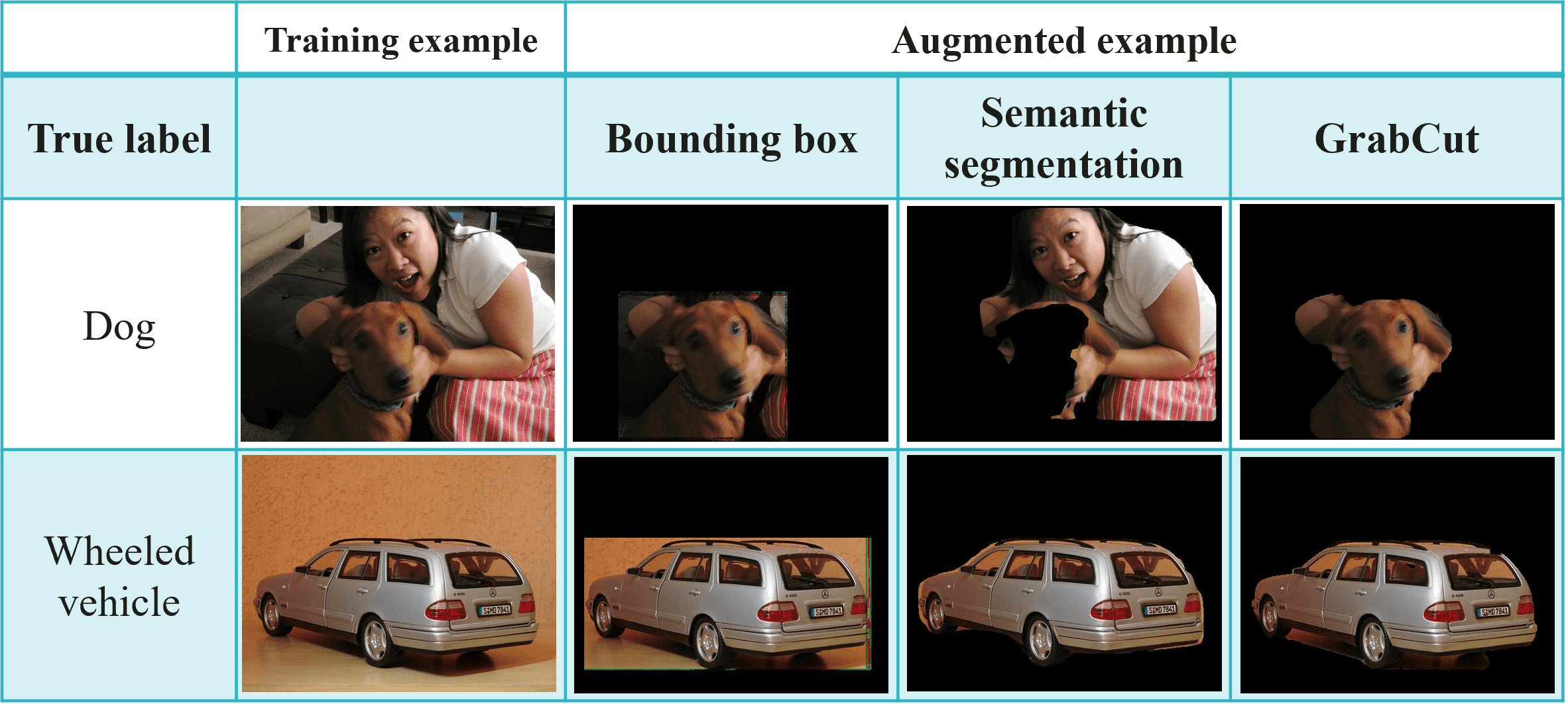
In this paper, we study a third lesser-known setting where a training domain is associated with a collection of pairs of examples that share the same semantic information. Such semantic sharing (SS) pairs can be created effortlessly using existing data augmentation (DA) methods, as demonstrated by the examples in Figure 1. Given a collection of SS pairs, the task is then to use them to reduce the dependence on spurious correlations.111At a high level of abstraction, this task is related to large language model (LLM) alignment where a collection of preference pairs is used to align an LLM to human intent [Ouyang et al., 2022b, Rafailov et al., 2023]. In both tasks, the pairs contain information about ideal model behavior that is absent from the training data. In this sense, one might say that what SS pairs is to domain generalization that preference pairs are to LLM alignment. There are several previous DG methods that exploit SS pairs for this purpose [Hendrycks et al., 2020, Mitrovic et al., 2021, Heinze-Deml and Meinshausen, 2021, Mahajan et al., 2021, Robey et al., 2021, Ouyang et al., 2021, Wang et al., 2022c]. They leverage SS pairs via consistency regularization (CR), a technique proposed in the semi-supervised learning literature to encourage similar predictions on similar inputs [Bachman et al., 2014, Zhang et al., 2020, Chen et al., 2020, Caron et al., 2021]. One drawback they share is that they regard an SS pair as unlabeled and assume and contain the same semantic information for all classes. As illustrated in Figure 1, however, an SS pair is often created to preserve the semantic information of one particular class, and is hence labeled. In this paper, we mainly study the use of labeled SS pairs for domain generalization.
We make three contributions in this paper: 1). We present a theory to motivate the use of SS pairs for optimal domain generalization through causally invariant prediction; 2). We propose a novel method called Logit Attribution Matching (LAM) that leverages labeled SS pairs; 3). We empirically demonstrate the advantages of LAM over representative single-source and multi-source DG methods, as well as various CR methods that leverage unlabeled SS pairs.
LAM consistently outperforms previous methods across multiple benchmarks. Take the iWildCam2020 dataset [Koh et al., 2021] as an example. ERM achieves OOD (Macro F1) score on an ImageNet pretrained ResNet-50 model [He et al., 2016]. The score increases to when the augmented examples created by RandAugment [Cubuk et al., 2020] are simply added to the training set. It further increases to when LAM is applied to the resulting SS pairs. For the augmented examples created by a more sophisticated data augmentation method [Gao et al., 2023], the OOD score is when the augmented examples are simply added to the training set. It further increases to when LAM is applied to the resulting SS pairs. In this case, the OOD performance increases by , with due to the exploitation of SS pairs. On CLIP ViT-L/14@336 [Radford et al., 2021], LAM improves the state-of-the-art fine-tuning method from to . It is hoped that our work can inspire the development of better SS pair creation methods so as to further boost OOD performance of models.
2 Related Work
Domain generalization (DG) is a fundamental problem in machine learning and has attracted much attention in recent years. A large number of methods have been proposed. In this section, we briefly review several representative methods that are frequently used as baselines in the literature. They are also used in our experiments as baselines.
Most DG methods assume access to multiple training domains [Blanchard et al., 2011, Muandet et al., 2013]. Among those multi-source methods, Group Distributionally Robust Optimization (GDRO) [Sagawa et al., 2020] seeks to minimize the worst-case risk across all possible training domains. Invariant Risk Minimization (IRM) [Arjovsky et al., 2019] regularizes ERM with a penalty that enforces cross-domain optimality on the classifier. Variance Risk Extrapolation (V-REx) [Krueger et al., 2020] penalizes the variance of risks in different training domains. Domain-Adversarial Neural Networks (DANN) [Ganin et al., 2016] aims at mapping inputs from each training domain to an invariant distribution in the feature space from which the original domains are indistinguishable.
Single-source DG does not assume access to multiple training domains [Volpi et al., 2018, Hendrycks and Dietterich, 2019]. One of the main approaches to single-source DG is to discover predictive features that are more sophisticated than simple cues spuriously correlated with labels. Representation Self-Challenging (RSC) [Huang et al., 2020] and Spectral Decoupling (SD) [Pezeshki et al., 2021] are two prominent methods in this direction. SD suppresses strong dependencies of output on dominant features by regularizing the logits. RSC aims to achieve the same goal in a heuristic manner. Another approach to single-source DG is to simply add augmented examples to the training set [Zhang et al., 2017, Cubuk et al., 2020, Gao et al., 2023]. This approach has been shown to improve OOD performance in many cases, because data augmentation exposes a model to more feature variations during training and thereby enhances its capability in dealing with novel domains.
Consistency regularization (CR) and semantic sharing (SS) pair creation.
CR encourages a model to make similar predictions on similar inputs. The idea originated from the semi-supervised learning literature [Bachman et al., 2014, Sohn et al., 2020]. It is also used in contrastive learning [Chen et al., 2020] and non-contrastive self-supervised learning [Caron et al., 2021]. In the context of DG, Wang et al. [2022a] conducted a systematic evaluation of various pre-existing CR methods and found that logit matching is most effective with -norm (among -norm, cosine similarity, etc.). In addition to logit matching with -norm, we study a few other options including novel ones such as target-logit matching and LAM which will be discussed in Section 4.1.
To apply CR in the context of DG, we need semantic sharing (SS) pairs. A straightforward way to create SS pairs is to use generic data augmentation (DA) techniques like CutMix [Yun et al., 2019] and RandAugment [Cubuk et al., 2020]. Previous CR methods primarily adopted generic DA techniques [Hendrycks et al., 2020, Xie et al., 2020, Wang et al., 2022a, Chen et al., 2022, Jing et al., 2023, Berezovskiy and Morozov, 2023]. SS pairs can also be created/obtained in ways other than conventional DA. For example, Gao et al. [2023] explored targeted data augmentation (Targeted DA) which utilizes task-specific domain knowledge to augment data. Heinze-Deml and Meinshausen [2021] paired up photos of the same person when analyzing the CelebA dataset [Liu et al., 2015]. For medical images, Ouyang et al. [2022a] created pairs by performing image transformations to simulate different possible acquisition processes. Furthermore, in the case of multiple source domains, SS pairs can be learned. Robey et al. [2021] and Wang et al. [2022c] build image-to-image translation networks between domains and use them to create pairs. Mahajan et al. [2021] propose an iterative algorithm that uses contrastive learning to map images to a latent space, and then match up images from different domains that have the same class label and are close to each other in the latent space.
3 A Causal Theory of Domain Generalization
In this section, we present a causal theory of domain generalization, which will be used in the next section to motivate methods for leveraging SS pairs. In the context of DG, a domain is defined by a distribution over the space of input-label pairs . We assume the pairs are generated by the causal model shown in Figure 2.
The model first appeared in Tenenbaum and Freeman [1996], where it is called the style and content decomposition (SCD) model, and and are called the content and style variables respectively. Similar models appeared recently in a number of papers under different terminologies. The variable denotes the essential information in an image that a human relies on to assign a label to the image. It is hence said to represent causal factors [Mahajan et al., 2021, Lv et al., 2022, Ye et al., 2022], intended factors [Geirhos et al., 2020], semantic factors [Liu et al., 2021], content factors [Mitrovic et al., 2021], and core factors [Heinze-Deml and Meinshausen, 2021]. In contrast, the variable denotes the other aspects of that are not essential to label assignment. It is hence said to represent non-causal factors, non-intended factors, variation factors, style factors, and non-core factors. As the relationship between and does not change across domains, is sometimes said to represent stable features [Zhang et al., 2021], domain-independent factors [Ouyang et al., 2022a], and invariant features [Arjovsky et al., 2019, Ahuja et al., 2021]. In contrast, is said to represent non-stable features, domain-dependent factors, and spurious features.
The term “style” in the SCD model should be understood in a broad sense. In addition to image style, it also includes factors such as background, context, object pose and so on. To avoid confusion, we follow Mahajan et al. [2021], Lv et al. [2022] and refer to and as the causal and non-causal factors respectively, and rename the SCD model as the causal latent decomposition (CLD) model.
To ground the CLD model, we need to specify three distributions: , and . Together, the three distributions define a joint distribution over the four variables:
This joint distribution defines a domain in the CLD framework. We refer to the collection of all such domains for some fixed and as a CLD family.
Let and be the sets of all possible values of the latent variables and respectively. Consider an example generated by from a pair of values 222We use upper case letters to denote variables and lower case letters to denote their values. We use with variables, e.g., , to denote a distribution; and with variable values, e.g., , to denote a probability value. We may omit the variables if the context is clear, e.g., we may write as . . Let be another example sampled from the same and a different . The two examples and contain the same semantic contents and hence should be classified into the same class. In this sense, and make up a semantic sharing (SS) pair. Let be a prediction model with parameters . It is said to be causally invariant if
| (1) |
for all SS pairs . In other words, the prediction output does not change in response to variations in the non-causal factors as long as the causal factors remain fixed. Such causal invariance is a key condition for optimal DG.
Theorem 1
(Conditions for Optimal DG) Let be a prediction model for a CLD family such that different almost always generate different , and let and be a source and a target domain (from the family) such that . Suppose:
-
1).
minimizes the in-distribution (ID) cross-entropy loss ;
-
2).
is causally invariant.
Then, the prediction model also minimizes the out-of-distribution (OOD) cross-entropy loss:
In other words, it generalizes optimally to the target domain.
The proof of this theorem can be found in Appendix A. Closely related theoretical results [Peters et al., 2016, Arjovsky et al., 2019, Mahajan et al., 2021] are discussed in Appendix B. The support consists of all causal factors that appear in a domain . The assumption on the support between and can be relaxed if we consider approximately optimal DG. We opt for simplicity here since it is not pertinent to the focus of this paper. More importantly, the second condition on connects consistency regularization (CR) with DG.
The intuition behind Theorem 1 is illustrated in Figure 3. In short, Theorem 1 articulates a set of sufficient conditions for optimal DG. While the causal invariance condition is difficult to verify or fully attain in practice, it can still guide the development of practical DG algorithms. We next discuss CR methods that can bring the model closer to meeting the causal invariance condition.
4 Consistency Regularization for Domain Generalization
Intuitively, one can make a model more causally invariant by encouraging the model to yield invariant predictions for SS pairs sharing the same . So, here is the problem we address in this paper:
Given a source domain from a CLD family and a set of labeled SS pairs , learn a prediction model that performs well in any target domain from the same CLD family.
Recall that a CLD family consists of all the domains defined by the causal model in Figure 2 with fixed and .
4.1 CR with Unlabeled SS Pairs
Let us first consider the case where we have a set of unlabeled SS pairs . The distinction between labeled and unlabeled SS pairs is if the semantic information is invariant for just one particular class or all classes, not whether the original examples is labeled. Unlabeled SS pairs contain stronger information than labeled SS pairs: two examples and contain the same semantic information for all classes implies that they contain the same semantic information for every class.
With unlabeled SS pairs, the first two conditions of Theorem 1 can be approximately satisfied by solving the following constrained optimization problem:
Of course, how well the two conditions are actually satisfied depends on how representative the unlabeled SS pairs we have are of all possible SS pairs.
If we turn the equality constraints into a consistency regularization (CR) term, the problem becomes:
where is a balancing parameter and the summation over is a regularization term that relaxes the corresponding equality constraints.
Some notations are needed in order to discuss specific choices for . Suppose consists of a feature extractor with parameters and a linear classification head with parameters . Hence, . For an input , let be the component of the feature vector for a feature unit . Let be the weight between a feature unit and the output unit for a class . The logit for class is
where the summation is over all feature units and the bias is omitted.
For each unlabeled SS pair , the CR term can be defined in several ways:
The first two terms aim to match the output probability distributions of and by minimizing either the KL or JS divergence between them. The third term aims to match their logit vectors, and the fourth term aims to match their feature vectors. They are used in previous methods ReLIC [Mitrovic et al., 2021], AugMix [Hendrycks et al., 2020], CoRE [Heinze-Deml and Meinshausen, 2021], and MatchDG [Mahajan et al., 2021] respectively. Note that while we focus on pairs for simplicity, logit and feature matching can also be extended to the case of multiple examples that share the same semantic contents. To achieve this, we can simply replace the sum of squared differences with the sum of variances. This is done in CoRE and MatchDG.
4.2 CR with labeled SS Pairs
Now consider the case where we have a set of labeled SS pairs . Here, each pair and share the same semantic information only for the class . It is no longer justifiable to match all the features, logits or probabilities of all classes. In the following, we propose three methods for leveraging labeled SS pairs.
First, we can match the probabilities or logits of the target class only, leading to what we call target probability matching (TPM) and target logit matching (TLM):
To introduce the third method, note that is the contribution to the logit of from the feature unit . We can match the logit contributions and from all feature units to . This gives rise to logit attribution matching (LAM):
LAM is of finer grain than TLM. Small implies small , but not vice versa:
where is the number of feature units. Also, note that
Hence, LAM exerts two complementary regularization forces, one on and the other on :
-
1).
It encourages the classification head to put large weights on the feature units where the values of and are similar, i.e., . In other words, it makes rely on the feature units that reflect the common information contents of and .
-
2).
It encourages the feature extractor to make for those feature units that relies on heavily, i.e., with large weights . In other words, it encourages to channel the common information contents of and toward the units that considers important.
As and share the causal factors for class but not the non-causal factors, those forces help a model focus more on the causal factors.
5 Experiments
A direct way to use augmented examples is to add them to the training set and train a model on the combined data using ERM. We denote this approach as ERM+DA. Alternatively, we can pair them up with the original images and apply CR methods on the resulting SS pairs. The main objective of our empirical studies is to compare LAM with ERM+DA, with ERM itself as a baseline. We also compare LAM with TPM and TLM, as well as previous CR methods.
Another way to utilize the augmented examples is to run a single-source DG algorithm on the combined data. It is also possible to treat the augmented examples as a separate domain and run a multi-source DG algorithm. We further compare LAM with representative single-source and multi-source DG methods in those settings.
Additionally, we assess the impact of the quality and quantity of augmented examples. We consider examples from two DA methods. The first one is RandAugment [Cubuk et al., 2020]. It creates augmented examples by applying a random set of transformations such as resizing, rotating, and color jittering to original images. The second method is Targeted DA [Gao et al., 2023]. It aims to randomize spurious factors while preserving robustly predictive factors. The specific designs of Targeted DA vary across datasets. Targeted DA generally yields more informative SS pairs infused with more specific domain knowledge. We call examples produced from Targeted DA target-augmented examples.
ImageNet-9 NICO PACS iWildCam Camelyon Average (CLIP ViT-B/16) (CLIP ViT-B/16) (CLIP ResNet-50) (ImageNet ResNet-50) (DenseNet-121) ERM 83.31.1 95.30.1 82.80.5 30.20.3 65.22.6 71.4 RandAugment ERM+DA 85.30.2 96.00.2 83.30.3 33.80.4 84.32.3 76.6 LAM 85.60.2 96.10.1 83.80.4 36.40.2 89.01.9 78.2 Targeted DA ERM+DA 86.01.0 95.90.3 84.50.5 36.50.4 90.50.9 78.7 LAM 88.10.2 96.50.3 86.00.3 41.20.2 93.51.8 81.1

5.1 Datasets
Our experiments involve five DG datasets, three with background shifts and two with style shifts.
iWildCam2020 (iWildCam) [Beery et al., 2020, Koh et al., 2021] consists of camera trap photos of animals taken at different locations for wildlife classification. The training domain comprises images from 200 locations, while the test and validation domains contain images from some other locations. Targeted DA is performed by Copy-Paste the animals in a training image to another image (with no animal) taken at a different location where the same animals sometimes appear [Gao et al., 2023].
ImageNet-9 [Xiao et al., 2020] includes images of nine coarse-grain classes from ImageNet [Deng et al., 2009]. Several synthetic variations are created by segmenting the foreground of each image and place it onto a different background. In our experiments, the synthetic images with a black background are used as target-augmented examples. For the test domain, we use the samples where the foreground of an original image is placed onto the background of a random image.
NICO [He et al., 2020] includes around 25,000 images across 19 classes of animals or vehicles in different contexts such as “at home” or “on the beach”. As there is no predefined train-test split, we randomly select one context per class for testing and use the remaining contexts for training. Target-augmented training examples and test domains are created in a way similar to ImageNet-9.
Camelyon17 (Camelyon) [Tellez et al., 2018, Koh et al., 2021] contains histopathology images from multiple hospitals for binary tumor classification. Images from three hospitals are used for training, while images from two other hospitals are used for testing and validation respectively. There are stylistic variations among images from different hospitals. One key stylistic difference often observed is the stain color. Therefore, the stain color jitter is applied to training images to create target-augmented examples [Gao et al., 2023].
PACS [Li et al., 2017] contains images of objects and creatures in four different styles: photo, art, cartoon and sketch. Following common practice [Li et al., 2017, Gulrajani and Lopez-Paz, 2021], we train a model using three of the domains and test the model on the fourth domain. For Targeted DA, we apply Stable Diffusion [Rombach et al., 2022] to images in the photo domain to create target-augmented examples in the other three domains. The photo domain is therefore not used as the test domain, while the other three domains are used as the test domain in turn. See Appendix C for details.
For all datasets, RandAugment [Cubuk et al., 2020] is performed on all training examples. Targeted DA [Gao et al., 2023] is also performed on all training examples in iWildCam and Camelyon. However, it is performed on only about 5% of the training data in ImageNet-9 and NICO, and about 10% of the training data for PACS.
All CR methods have a balancing parameter , which is tuned on the validation domain for iWildCam and Camelyon, and on a test set from the training domain for the other three datasets. For CR and single-source methods, multiple training domains are simply combined into one. More details on how the training data are organized for different types of methods can be found in Table 5 (Appendix E).
5.2 Network Architecture and Weight Initialization
Following Gao et al. [2023], we use a variety of models for different datasets. Specifically, we use an ImageNet pretrained ResNet-50 model [He et al., 2016] for iWildCam, and a randomly initialized DenseNet-121 model [Huang et al., 2017] for Camelyon. We use a CLIP-pretrained ViT-B/16 model [Radford et al., 2021] for ImageNet-9 and NICO, and a CLIP-pretrained ResNet-50 model for PACS.
To showcase the combined use of LAM with advanced CLIP model fine-tuning method can yield SOTA-level performance on iWildCam, we also employ CLIP-pretrained ViT-L/14 and ViT-L/14@336 model for iWildCam.
The use of various model architectures and weight initializations allows us to assess the relative merits of DG algorithms on a mixture of datasets and models. Implementation details about hyperparameters for each dataset and method can also be found in Appendix E.
ImageNet-9 NICO PACS iWildCam Camelyon Average iWildCam-N RandAugment ERM+DA 85.30.2 – 96.00.2 – 83.30.3 – 33.80.4 – 84.32.3 – 76.6 – 27.60.5 – KL 85.20.3 96.00.2 – 83.10.4 34.80.2 86.75.5 77.2 27.30.2 JS 85.20.1 95.70.5 82.71.4 34.50.3 83.46.7 76.3 26.60.4 LM 84.90.1 95.80.4 82.70.2 29.60.3 87.91.4 76.2 26.50.4 FM 85.20.1 96.20.1 82.31.0 31.80.3 81.75.3 75.4 26.20.3 TPM 85.40.1 96.20.5 82.50.6 34.30.2 86.94.3 77.1 28.00.2 TLM 85.30.1 – 95.10.3 82.40.5 34.10.4 87.23.2 76.8 27.90.4 LAM 85.60.2 96.10.1 83.80.4 36.40.2 89.01.9 78.2 28.40.2 Targeted DA ERM+DA 86.01.0 – 95.90.3 – 84.50.5 – 36.50.4 – 90.50.9 – 78.7 – 28.20.5 – KL 86.90.2 95.40.2 85.01.0 40.30.3 92.81.5 80.1 26.30.7 JS 86.00.4 – 95.00.3 84.30.3 37.10.4 94.81.2 79.4 25.50.6 LM 86.80.6 95.30.2 83.10.8 34.30.5 93.40.3 78.6 23.90.5 FM 87.60.1 95.50.2 81.70.2 36.00.3 94.30.6 79.0 25.30.7 TPM 86.70.1 95.80.2 84.80.7 38.40.2 91.71.9 79.5 28.30.4 TLM 86.20.2 95.90.2 – 85.31.5 38.50.3 93.90.7 80.0 28.80.2 LAM 88.10.2 96.50.3 86.00.3 41.20.2 93.51.8 81.1 29.80.3
5.3 Comparison with ERM+DA
Table 1 shows the results for LAM, ERM+DA, and ERM. We see that simply adding augmented data to the training set (ERM+DA) increases the average OOD score from 71.4% to 76.5% with RandAugment [Cubuk et al., 2020], and to 78.7% with Targeted DA [Gao et al., 2023]. Applying LAM on the resulting SS pairs further increases the scores to 78.2% and 81.1% in the two cases respectively. In the case of Targeted DA, the average OOD score on those five benchmarks is improved by 81.1-71.4 = 9.7%, with 78.7-71.4 = 7.3% due to data augmentation and 81.1-78.7 = 2.4% due to LAM. The improvements are especially pronounced on the iWildCam and Camelyon datasets, where Targeted DA increases the OOD scores drastically. This is consistent with what was reported in Gao et al. [2023]. LAM further improves the scores by 4.7% and 3.0% respectively.
While trying to gain some insights, we find that LAM makes a model focus on much fewer feature units (see Figure 11 in Appendix F) as compared with ERM+DA. We also use an XAI method called Grad-CAM [Selvaraju et al., 2017] to explain the outputs of the model trained on ImageNet-9 by LAM and they some other methods. Examples are shown in Figure 4 (and Figure 12 in Appendix F). We see that, in all those examples, the LAM model focuses on the foreground objects and gives the correct predictions. Those corroborate with the analysis we make at the end of Section 4.2. In contrast, the ERM+DA model is more inclined to focus on the wrong part of an input image and predict incorrectly.
In addition to comparing LAM over the traditional ERM which is based on the standard cross-entropy loss, it has been shown in Goyal et al. [2023] that when fine-tuning CLIP models, the use of CLIP contrastive loss with utilizing the CLIP text encoder is more effective. The proposed method is colloquially known as “finetune like you pretrain” (FLYP). In Table 3, we show that the use of LAM can also yield improved OOD performance over FLYP+DA.
5.4 Impact of Quality and Quantity of Augmented Examples
Both LAM and ERM+DA achieve better results with Targeted DA than with RandAugment. We believe this is because Targeted DA generally yields higher quality augmentations than the latter. To further support the claim, we perform additional experiments with ImageNet-9 in the Targeted DA setting. Specifically, we test three different ways to create augmented examples: 1). use a segmentation method called GrabCut [Rother et al., 2004], 2). use another less effective segmentation method called FCN [Long et al., 2015], and 3). simply use bounding boxes that come with ImageNet-9 (Box). The resulting OOD scores are as follows:
| Box | FCN | GrabCut | |||
|---|---|---|---|---|---|
| ERM+DA | LAM | ERM+DA | LAM | ERM+DA | LAM |
| 85.2 | 85.9 | 83.9 | 86.6 | 86.0 | 88.1 |
We see that, as expected, the results with GrabCut are the best, followed by those with FCN and Box, in that order.
We also perform additional experiments with ImageNet-9 to investigate how the quantity of augmented examples influences LAM. Specifically, GrabCut is applied to different percentages of the training examples and LAM is run on the resulting SS pairs. To make a comparison, we do the same thing for the ERM+DA. The resulting OOD scores are as follows:
| 5% | 10% | 20% | 50% | 100% | |
|---|---|---|---|---|---|
| ERM+DA | 86.0 | 86.9 | 86.1 | 87.4 | 87.8 |
| LAM | 88.1 | 88.5 | 88.6 | 89.7 | 90.4 |
It is clear that the increase in the quantity of SS pairs benefits LAM, and the availability of SS pairs for a small fraction of training examples can significantly improve OOD performance already. While providing more SS pairs can also improve the performance of ERM+DA, it is obvious that the improvement is smaller than that of LAM.
Model Method ID F1 OOD F1 CLIP- FLYP 56.9 43.4 ViT-L/14 FLYP+DA 59.0 44.3 FLYP+DA+LAM 59.0 45.6 CLIP- FLYP 59.9 46.0 ViT-L/14@336 FLYP+DA 58.9 47.1 FLYP+DA+LAM 60.9 48.7
ImageNet-9 NICO PACS iWildCam Camelyon Average ERM 83.31.1 95.30.1 82.80.5 30.20.3 65.22.6 71.4 ERM+DA 86.01.0 – 95.90.3 – 84.50.5 – 36.50.4 – 90.50.9 – 78.7 – Single-source RSC 86.40.2 94.01.8 84.30.6 32.70.9 91.60.3 77.8 SD 86.70.3 96.00.2 85.00.4 32.70.8 93.50.5 78.8 Multi-source DANN 86.50.7 95.40.7 77.91.1 26.02.9 90.10.9 75.2 GDRO 83.70.8 91.81.2 83.50.5 37.01.0 92.20.9 77.6 IRM 87.10.2 93.50.2 83.20.4 31.70.1 90.82.6 77.3 V-REx 83.61.4 94.00.9 84.40.2 35.61.6 90.44.1 77.6 LAM 88.10.2 96.50.3 86.00.3 41.20.2 93.51.8 81.1
5.5 Comparison with Other CR Methods
Table 2 shows the results for LAM and other CR methods. Let us first compare LAM and two other CR methods we propose in this paper, namely target probability matching (TPM) and target logit matching (TLM). We see that LAM achieves higher OOD scores than the other two methods on average, and it outperforms ERM+DA in all cases while the other two methods do not. Those show that when making use of labeled SS pairs, it is more effective to apply consistency regularization to the logit contributions of the target classes (LAM) rather than the logits themselves (TLM) or the probabilities of the target classes (TPM).
Next, we compare LAM with previous strong CR methods, namely probability matching with KL or JS, logit matching (LM) and feature matching (FM). LAM achieves higher OOD scores than those methods on average. Moreover, it achieves the highest score in all cases except for Camelyon with Targeted DA. Moreover, it outperforms ERM+DA in all cases, while the other methods do not. Those show that it is generally beneficial to regard SS pairs created using both Targeted DA and RandAugment as labeled and apply LAM on them, rather than considering them unlabeled and applying any of the previous CR methods on them.
In LAM, a labeled SS pair is used only to regularize the contributions from feature units to the logit of the ground-truth class . It does not impact the other classes. In the previous CR methods, on the other hand, the pair is used to regularize the entire feature, logit, or probability vector for . It affects other classes as well as . This is problematic when a training example contains multiple objects of interest. Some objects that appear in the background of the main object in might be removed during data augmentation. In such a case, the features of those minor objects would be suppressed. To further demonstrate the adverse consequences, we created a variant of the iWildCam dataset [Beery et al., 2020, Koh et al., 2021] by adding a small segmented image of another animal to the background of each image. The new dataset is named iWildCam-N (examples of this dataset are given in Appendix D). On this dataset, LAM still improves over ERM+DA. However, the performances of all four previous methods are substantially worse than that of ERM+DA.
Camelyon is a binary classification problem. There is no issue of suppressing features of other classes. This is probably why probability matching with JS is superior to LAM on Camelyon in the case of Targeted DA.
5.6 Comparison with Other DG Methods
Table 4 shows the OOD performances of LAM with six representative single-source and multi-source DG methods reviewed in Section 2. Here only Targeted DA [Gao et al., 2023] is considered. On the first four datasets, LAM outperforms all the six DG methods on average. In particular, it outperforms them by large margins on iWildCam. While LAM improves over ERM+DA on all the first four datasets, the other methods are inferior to ERM+DA in the majority of the cases. On the binary classification dataset Camelyon, however, LAM is on par with SD [Pezeshki et al., 2021], but it still outperforms ERM+DA.
Recall that augmented examples are simply added to the training set for the single-source methods (RSC [Huang et al., 2020] and SD), and they are treated as an additional training domain for the multi-sources methods (DANN [Ganin et al., 2016], GDRO [Sagawa et al., 2020], IRM [Arjovsky et al., 2019] and V-REx [Krueger et al., 2020]). In contrast, LAM applies consistency regularization on the resulting SS pairs. The results in Table 4 show that consistency regularization with LAM is a more effective way to use augmented examples than representative previous single-source and multi-source DG methods.
6 Conclusion
In this paper, we study the setting where a training domain is associated with a collection of example pairs that share the same semantic information. We present a theory to motivate using such semantic sharing (SS) pairs to boost model robustness under domain shift. We find that applying consistency regularization (CR) on the SS pairs, particularly using LAM, significantly improves OOD performance compared to simply adding the augmented examples to the training set. An interesting future direction is to develop more efficient methods for creating more informative SS pairs, e.g., by leveraging advances in generative models. We hope our work could encourage more efforts in manually creating SS pairs for domain generalization, similar to the collection of human preference pairs for LLM alignment.
Acknowledgement
We thank the deep learning computing framework MindSpore (https://www.mindspore.cn) and its team for the support on this work. Research on this paper was supported in part by Hong Kong Research Grants Council under grant 16204920. Kaican Li and Weiyan Xie were supported in part by the Huawei PhD Fellowship Scheme.
References
- Ahuja et al. [2021] Kartik Ahuja, Ethan Caballero, Dinghuai Zhang, Jean-Christophe Gagnon-Audet, Yoshua Bengio, Ioannis Mitliagkas, and Irina Rish. Invariance principle meets information bottleneck for out-of-distribution generalization. In NeurIPS, volume 34, pages 3438–3450, 2021.
- Alcorn et al. [2019] Michael A Alcorn, Qi Li, Zhitao Gong, Chengfei Wang, Long Mai, Wei-Shinn Ku, and Anh Nguyen. Strike (with) a pose: Neural networks are easily fooled by strange poses of familiar objects. In CVPR, 2019.
- Ali et al. [2022] Sharib Ali, Noha Ghatwary, Debesh Jha, Ece Isik-Polat, Gorkem Polat, Chen Yang, Wuyang Li, Adrian Galdran, Miguel-Ángel González Ballester, Vajira Thambawita, et al. Assessing generalisability of deep learning-based polyp detection and segmentation methods through a computer vision challenge. arXiv:2202.12031, 2022.
- Arjovsky [2020] Martin Arjovsky. Out of distribution generalization in machine learning. PhD thesis, New York University, 2020.
- Arjovsky et al. [2019] Martin Arjovsky, Léon Bottou, Ishaan Gulrajani, and David Lopez-Paz. Invariant risk minimization. arXiv:1907.02893, 2019.
- Bachman et al. [2014] Philip Bachman, Ouais Alsharif, and Doina Precup. Learning with pseudo-ensembles. In NeurIPS, volume 27, 2014.
- Beery et al. [2018] Sara Beery, Grant Van Horn, and Pietro Perona. Recognition in terra incognita. In ECCV, 2018.
- Beery et al. [2020] Sara Beery, Elijah Cole, and Arvi Gjoka. The iWildCam 2020 competition dataset. arXiv:2004.10340, 2020.
- Beery et al. [2021] Sara Beery, Arushi Agarwal, Elijah Cole, and Vighnesh Birodkar. The iWildCam 2021 competition dataset. arXiv:2105.03494, 2021.
- Ben-David et al. [2010] Shai Ben-David, John Blitzer, Koby Crammer, Alex Kulesza, Fernando Pereira, and Jennifer Wortman Vaughan. A theory of learning from different domains. Machine learning, 79:151–175, 2010.
- Berezovskiy and Morozov [2023] Valeriy Berezovskiy and Nikita Morozov. Weight averaging improves knowledge distillation under domain shift. arXiv:2309.11446, 2023.
- Blanchard et al. [2011] Gilles Blanchard, Gyemin Lee, and Clayton Scott. Generalizing from several related classification tasks to a new unlabeled sample. In NeurIPS, 2011.
- Caron et al. [2021] Mathilde Caron, Hugo Touvron, Ishan Misra, Hervé Jégou, Julien Mairal, Piotr Bojanowski, and Armand Joulin. Emerging properties in self-supervised vision transformers. In ICCV, pages 9650–9660, 2021.
- Chen et al. [2022] Dian Chen, Dequan Wang, Trevor Darrell, and Sayna Ebrahimi. Contrastive test-time adaptation. In CVPR, pages 295–305, 2022.
- Chen et al. [2020] Ting Chen, Simon Kornblith, Mohammad Norouzi, and Geoffrey Hinton. A simple framework for contrastive learning of visual representations. In ICML, pages 1597–1607. PMLR, 2020.
- Cubuk et al. [2020] Ekin D Cubuk, Barret Zoph, Jonathon Shlens, and Quoc V Le. RandAugment: Practical automated data augmentation with a reduced search space. In CVPR workshops, pages 702–703, 2020.
- Deng et al. [2009] Jia Deng, Wei Dong, Richard Socher, Li-Jia Li, Kai Li, and Li Fei-Fei. ImageNet: A large-scale hierarchical image database. In CVPR, 2009.
- Di Langosco et al. [2022] Lauro Langosco Di Langosco, Jack Koch, Lee D Sharkey, Jacob Pfau, and David Krueger. Goal misgeneralization in deep reinforcement learning. In ICML, pages 12004–12019. PMLR, 2022.
- Ganin et al. [2016] Yaroslav Ganin, Evgeniya Ustinova, Hana Ajakan, Pascal Germain, Hugo Larochelle, François Laviolette, Mario Marchand, and Victor Lempitsky. Domain-adversarial training of neural networks. JMLR, 2016.
- Gao et al. [2023] Irena Gao, Shiori Sagawa, Pang Wei Koh, Tatsunori Hashimoto, and Percy Liang. Out-of-domain robustness via targeted augmentations. In ICML, 2023.
- Geirhos et al. [2020] Robert Geirhos, Jörn-Henrik Jacobsen, Claudio Michaelis, Richard Zemel, Wieland Brendel, Matthias Bethge, and Felix A. Wichmann. Shortcut learning in deep neural networks. Nature Machine Intelligence, 2020.
- Goyal et al. [2023] Sachin Goyal, Ananya Kumar, Sankalp Garg, Zico Kolter, and Aditi Raghunathan. Finetune like you pretrain: Improved finetuning of zero-shot vision models. In CVPR, pages 19338–19347, 2023.
- Gulrajani and Lopez-Paz [2021] Ishaan Gulrajani and David Lopez-Paz. In search of lost domain generalization. In ICLR, 2021.
- He et al. [2016] Kaiming He, Xiangyu Zhang, Shaoqing Ren, and Jian Sun. Deep residual learning for image recognition. In CVPR, 2016.
- He et al. [2020] Yue He, Zheyan Shen, and Peng Cui. Towards non-IID image classification: A dataset and baselines. Pattern Recognition, 2020.
- Heinze-Deml and Meinshausen [2021] Christina Heinze-Deml and Nicolai Meinshausen. Conditional variance penalties and domain shift robustness. Machine Learning, 110(2):303–348, 2021.
- Hendrycks and Dietterich [2019] Dan Hendrycks and Thomas Dietterich. Benchmarking neural network robustness to common corruptions and perturbations. In ICLR, 2019.
- Hendrycks et al. [2020] Dan Hendrycks, Norman Mu, Ekin D. Cubuk, Barret Zoph, Justin Gilmer, and Balaji Lakshminarayanan. AugMix: A simple data processing method to improve robustness and uncertainty. In ICLR, 2020.
- Huang et al. [2017] Gao Huang, Zhuang Liu, Laurens Van Der Maaten, and Kilian Q Weinberger. Densely connected convolutional networks. In CVPR, pages 4700–4708, 2017.
- Huang et al. [2020] Zeyi Huang, Haohan Wang, Eric P Xing, and Dong Huang. Self-challenging improves cross-domain generalization. In ECCV, pages 124–140. Springer, 2020.
- Jing et al. [2023] Mengmeng Jing, Xiantong Zhen, Jingjing Li, and Cees GM Snoek. Order-preserving consistency regularization for domain adaptation and generalization. In ICCV, pages 18916–18927, 2023.
- Koh et al. [2021] Pang Wei Koh, Shiori Sagawa, Henrik Marklund, Sang Michael Xie, Marvin Zhang, Akshay Balsubramani, Weihua Hu, Michihiro Yasunaga, Richard Lanas Phillips, Irena Gao, et al. Wilds: A benchmark of in-the-wild distribution shifts. In ICML, pages 5637–5664. PMLR, 2021.
- Krueger et al. [2020] David Krueger, Ethan Caballero, Joern-Henrik Jacobsen, Amy Zhang, Jonathan Binas, Remi Le Priol, and Aaron Courville. Out-of-distribution generalization via risk extrapolation (REx). arXiv:2003.00688, 2020.
- Kumar et al. [2022] Ananya Kumar, Aditi Raghunathan, Robbie Jones, Tengyu Ma, and Percy Liang. Fine-tuning can distort pretrained features and underperform out-of-distribution. arXiv:2202.10054, 2022.
- Li et al. [2017] D. Li, Y. Yang, Y. Song, and T. M. Hospedales. Deeper, broader and artier domain generalization. In ICCV, 2017.
- Li et al. [2022] Kaican Li, Kai Chen, Haoyu Wang, Lanqing Hong, Chaoqiang Ye, Jianhua Han, Yukuai Chen, Wei Zhang, Chunjing Xu, Dit-Yan Yeung, et al. Coda: A real-world road corner case dataset for object detection in autonomous driving. In ECCV, pages 406–423. Springer, 2022.
- Liu et al. [2021] Chang Liu, Xinwei Sun, Jindong Wang, Haoyue Tang, Tao Li, Tao Qin, Wei Chen, and Tie-Yan Liu. Learning causal semantic representation for out-of-distribution prediction. In NeurIPS, 2021.
- Liu et al. [2020] Hong Liu, Pinhao Song, and Runwei Ding. Towards domain generalization in underwater object detection. In ICIP, pages 1971–1975. IEEE, 2020.
- Liu et al. [2015] Ziwei Liu, Ping Luo, Xiaogang Wang, and Xiaoou Tang. Deep learning face attributes in the wild. In ICCV, 2015.
- Long et al. [2015] Jonathan Long, Evan Shelhamer, and Trevor Darrell. Fully convolutional networks for semantic segmentation. In CVPR, pages 3431–3440, 2015.
- Lv et al. [2022] Fangrui Lv, Jian Liang, Shuang Li, Bin Zang, Chi Harold Liu, Ziteng Wang, and Di Liu. Causality inspired representation learning for domain generalization. In CVPR, pages 8046–8056, 2022.
- Mahajan et al. [2021] Divyat Mahajan, Shruti Tople, and Amit Sharma. Domain generalization using causal matching. In ICML, pages 7313–7324. PMLR, 2021.
- Michaelis et al. [2019] Claudio Michaelis, Benjamin Mitzkus, Robert Geirhos, Evgenia Rusak, Oliver Bringmann, Alexander S Ecker, Matthias Bethge, and Wieland Brendel. Benchmarking robustness in object detection: Autonomous driving when winter is coming. arXiv:1907.07484, 2019.
- Mitrovic et al. [2021] Jovana Mitrovic, Brian McWilliams, Jacob C Walker, Lars Holger Buesing, and Charles Blundell. Representation learning via invariant causal Mechanisms. In ICLR, 2021.
- Muandet et al. [2013] Krikamol Muandet, David Balduzzi, and Bernhard Schölkopf. Domain generalization via invariant feature representation. In ICML, 2013.
- Ouyang et al. [2021] Cheng Ouyang, Chen Chen, Surui Li, Zeju Li, Chen Qin, Wenjia Bai, and Daniel Rueckert. Causality-inspired single-source domain generalization for medical image segmentation. arXiv:2111.12525, 2021.
- Ouyang et al. [2022a] Cheng Ouyang, Chen Chen, Surui Li, Zeju Li, Chen Qin, Wenjia Bai, and Daniel Rueckert. Causality-inspired single-source domain generalization for medical image segmentation. IEEE Transactions on Medical Imaging, 2022a.
- Ouyang et al. [2022b] Long Ouyang, Jeffrey Wu, Xu Jiang, Diogo Almeida, Carroll Wainwright, Pamela Mishkin, Chong Zhang, Sandhini Agarwal, Katarina Slama, Alex Ray, et al. Training language models to follow instructions with human feedback. In NeurIPS, volume 35, pages 27730–27744, 2022b.
- Peters et al. [2016] Jonas Peters, Peter Bühlmann, and Nicolai Meinshausen. Causal inference by using invariant prediction: identification and confidence intervals. Journal of the Royal Statistical Society: Series B (Statistical Methodology), 78(5):947–1012, 2016.
- Pezeshki et al. [2021] Mohammad Pezeshki, Oumar Kaba, Yoshua Bengio, Aaron C Courville, Doina Precup, and Guillaume Lajoie. Gradient starvation: A learning proclivity in neural networks. In NeurIPS, volume 34, pages 1256–1272, 2021.
- Radford et al. [2021] Alec Radford, Jong Wook Kim, Chris Hallacy, Aditya Ramesh, Gabriel Goh, Sandhini Agarwal, Girish Sastry, Amanda Askell, Pamela Mishkin, Jack Clark, et al. Learning transferable visual models from natural language supervision. In ICML, pages 8748–8763. PMLR, 2021.
- Rafailov et al. [2023] Rafael Rafailov, Archit Sharma, Eric Mitchell, Stefano Ermon, Christopher D Manning, and Chelsea Finn. Direct preference optimization: Your language model is secretly a reward model. arXiv:2305.18290, 2023.
- Robey et al. [2021] Alexander Robey, George Pappas, and Hamed Hassani. Model-based domain generalization. In NeurIPS, 2021.
- Rombach et al. [2022] Robin Rombach, Andreas Blattmann, Dominik Lorenz, Patrick Esser, and Björn Ommer. High-resolution image synthesis with latent diffusion models. In CVPR, pages 10684–10695, 2022.
- Rother et al. [2004] Carsten Rother, Vladimir Kolmogorov, and Andrew Blake. “GrabCut” interactive foreground extraction using iterated graph cuts. ACM transactions on graphics (TOG), 23(3):309–314, 2004.
- Sagawa et al. [2020] Shiori Sagawa, Pang Wei Koh, Tatsunori B. Hashimoto, and Percy Liang. Distributionally Robust Neural Networks. In ICLR, 2020.
- Selvaraju et al. [2017] Ramprasaath R Selvaraju, Michael Cogswell, Abhishek Das, Ramakrishna Vedantam, Devi Parikh, and Dhruv Batra. Grad-CAM: Visual explanations from deep networks via gradient-based localization. In ICCV, pages 618–626, 2017.
- Shah et al. [2020] Harshay Shah, Kaustav Tamuly, Aditi Raghunathan, Prateek Jain, and Praneeth Netrapalli. The pitfalls of simplicity bias in neural networks. In NeurIPS, volume 33, pages 9573–9585, 2020.
- Sohn et al. [2020] Kihyuk Sohn, David Berthelot, Nicholas Carlini, Zizhao Zhang, Han Zhang, Colin A Raffel, Ekin Dogus Cubuk, Alexey Kurakin, and Chun-Liang Li. FixMatch: Simplifying semi-supervised learning with consistency and confidence. In NeurIPS, volume 33, pages 596–608, 2020.
- Szegedy et al. [2013] Christian Szegedy, Wojciech Zaremba, Ilya Sutskever, Joan Bruna, Dumitru Erhan, Ian Goodfellow, and Rob Fergus. Intriguing properties of neural networks. arXiv:1312.6199, 2013.
- Tellez et al. [2018] David Tellez, Maschenka Balkenhol, Irene Otte-Höller, Rob van de Loo, Rob Vogels, Peter Bult, Carla Wauters, Willem Vreuls, Suzanne Mol, Nico Karssemeijer, et al. Whole-slide mitosis detection in H&E breast histology using PHH3 as a reference to train distilled stain-invariant convolutional networks. IEEE transactions on medical imaging, 37(9):2126–2136, 2018.
- Tenenbaum and Freeman [1996] Joshua Tenenbaum and William Freeman. Separating style and content. In NeurIPS, volume 9, 1996.
- Volpi et al. [2018] Riccardo Volpi, Hongseok Namkoong, Ozan Sener, John C Duchi, Vittorio Murino, and Silvio Savarese. Generalizing to unseen domains via adversarial data augmentation. In NeurIPS, 2018.
- Wang et al. [2022a] Haohan Wang, Zeyi Huang, Xindi Wu, and Eric Xing. Toward learning robust and invariant representations with alignment regularization and data augmentation. In SIGKDD, pages 1846–1856, 2022a.
- Wang et al. [2022b] Jindong Wang, Cuiling Lan, Chang Liu, Yidong Ouyang, Tao Qin, Wang Lu, Yiqiang Chen, Wenjun Zeng, and Philip Yu. Generalizing to unseen domains: A survey on domain generalization. IEEE Transactions on Knowledge and Data Engineering, 2022b.
- Wang et al. [2022c] Ruoyu Wang, Mingyang Yi, Zhitang Chen, and Shengyu Zhu. Out-of-distribution generalization with causal invariant transformations. In CVPR, pages 375–385, 2022c.
- Wang et al. [2024] Yimu Wang, Yihan Wu, and Hongyang Zhang. Lost domain generalization is a natural consequence of lack of training domains. In AAAI, 2024.
- Xiao et al. [2020] Kai Xiao, Logan Engstrom, Andrew Ilyas, and Aleksander Madry. Noise or signal: The role of image backgrounds in object recognition. arXiv:2006.09994, 2020.
- Xie et al. [2020] Qizhe Xie, Zihang Dai, Eduard Hovy, Thang Luong, and Quoc Le. Unsupervised data augmentation for consistency training. In NeurIPS, volume 33, pages 6256–6268, 2020.
- Yang et al. [2023] Linyi Yang, Shuibai Zhang, Libo Qin, Yafu Li, Yidong Wang, Hanmeng Liu, Jindong Wang, Xing Xie, and Yue Zhang. Glue-x: Evaluating natural language understanding models from an out-of-distribution generalization perspective. In ACL, 2023.
- Ye et al. [2022] Nanyang Ye, Kaican Li, Haoyue Bai, Runpeng Yu, Lanqing Hong, Fengwei Zhou, Zhenguo Li, and Jun Zhu. Ood-bench: Quantifying and understanding two dimensions of out-of-distribution generalization. In CVPR, pages 7947–7958, 2022.
- Yun et al. [2019] Sangdoo Yun, Dongyoon Han, Seong Joon Oh, Sanghyuk Chun, Junsuk Choe, and Youngjoon Yoo. CutMix: Regularization strategy to train strong classifiers with localizable features. In ICCV, pages 6023–6032, 2019.
- Zech et al. [2018] John R Zech, Marcus A Badgeley, Manway Liu, Anthony B Costa, Joseph J Titano, and Eric Karl Oermann. Variable generalization performance of a deep learning model to detect pneumonia in chest radiographs: a cross-sectional study. PLoS medicine, 15(11):e1002683, 2018.
- Zhang et al. [2020] Han Zhang, Zizhao Zhang, Augustus Odena, and Honglak Lee. Consistency regularization for generative adversarial networks. In ICLR, 2020.
- Zhang et al. [2017] Hongyi Zhang, Moustapha Cisse, Yann N Dauphin, and David Lopez-Paz. mixup: Beyond empirical risk minimization. arXiv:1710.09412, 2017.
- Zhang et al. [2021] Xingxuan Zhang, Peng Cui, Renzhe Xu, Linjun Zhou, Yue He, and Zheyan Shen. Deep stable learning for out-of-distribution generalization. arXiv:2104.07876, 2021.
- Zhou et al. [2022] Kaiyang Zhou, Ziwei Liu, Yu Qiao, Tao Xiang, and Chen Change Loy. Domain generalization: A survey. IEEE Transactions on Pattern Analysis and Machine Intelligence, 2022.
Appendix A Proofs
Proof of Theorem 1: Let us start with the ID cross-entropy loss:
Because is causally invariant, depends only on , but not . Denote it as . Then, we get
As the ID loss is minimized, the inner expectation is maximized for any such that .
Now, consider the OOD cross-entropy loss of the target domain . By symmetry, we have:
We know from above that the inner expectation is maximized for all such that .
It is also maximized for any
such that because
.
Appendix B Related Theoretical Results
The concept of causally invariant prediction (CIP) that we introduce in Section 3 is closely related to a notion described in Peters et al. [2016] that bears a very similar name — invariant causal prediction (ICP). There is a subtle difference. causally invariant prediction refers to the situation where a model makes predictions based on causal factors and, consequently, its performance remains invariant across domains. On the other hand, invariant causal prediction refers to the situation where a model’s performance remains invariant across domains and, consequently, its input variables can be considered as causes for the output variable. CIP is for domain generalization while ICP is for causal discovery. In addition, our work involves latent variables ( and ) while Peters et al. [2016] deal with only observed variables.
Our Theorem 1 is closely related to Theorem 1 of Mahajan et al. [2021] and Theorem 3.2 of Arjovsky [2020]. However, the causal model used by Mahajan et al. [2021] has three more latent variables than the one we use. In fact, our model can be viewed as their model with the additional latent variables “integrated out”. As such, our theorem targets a more general setting. In addition, their theorem focuses exclusively on feature matching and hence cannot be used to motivate logit attribution matching (LAM). Arjovsky’s theorem also focuses on the feature extractor. It requires examples with the same feature representation to have approximately the same output probability distributions under the generative model. In this sense, it seeks to obtain features with invariant prediction by the generative model. In contrast, our theorem requires a prediction model to be invariant to the non-causal factors. While Arjovsky’s theorem is used to motivate a DG algorithm called invariant risk minimization (IRM), our theorem is used to justify consistency regularization.
In this paper, we use a causal theory of domain generalization to motivate consistency regularization methods. It should be noted that there are other theories for domain generalization that are based on divergence between domains [Ben-David et al., 2010, Liu et al., 2020]. Those theories are used to motivate the domain invariant representation approach to domain generalization. However, they cannot be used to justify consistency regularization methods.
Appendix C More details of SS pair creation using Targeted DA
An SS pair is formed by a training example and an augmented example. The SS pair creation using Targeted DA for each dataset has been introduced in Section 5.1. We provide more details and examples here.
C.1 iWildCam and iwildcam-N
For iWildCam and iWildCam-N, we utilized a Targeted DA technique named Copy-Paste (same-y) from Gao et al. [2023]. This DA method pastes the animal foreground onto a background image sampled from the same habitat where the same animal species has been observed. There is a category of images labeled “empty” in the iWildCam dataset. These images do not contain any animals and were used as background images when creating augmented examples. We used the segmentation for the animal foregrounds provided by Beery et al. [2021] to apply this DA. Augmented examples produced by this DA approach are provided in Figure 5.

C.2 ImageNet-9
In our main experiments, the synthetic images with a black background were used as augmented data for ImageNet-9. Those augmented examples were created based on the GrabCut segmentation. As described in Section 5.4, to assess the performance of LAM under augmented examples in various qualities, we also considered the augmented examples created based on the bounding boxes and semantic segmentation. Specifically, we used the bounding boxes provided by the ImageNet [Deng et al., 2009] and semantic segmentation produced via FCN [Long et al., 2015], a semantic segmentation method. Augmented examples in various qualities are given in Figure 6.
C.3 NICO
For creating the augmented examples for NICO, we placed the foreground segmentation onto the background of a random image. We used GrabCut [Rother et al., 2004] to identify the foreground segmentation for 20 images in each class of NICO, which constituted about 5% of its training data. On average, the segmentation of an image took us around three seconds.
Since NICO does not have “empty” background images like iWildCam, we had to create synthetic background images. To do this, we removed the foreground in the image by coloring the image region corresponding to the foreground segmentation in black. We created the synthetic background images for all images with the foreground segmentation. When creating the augmented example, the foreground segmentation in the training example is pasted onto a randomly selected synthetic background image. See Figure 7 for some NICO augmented examples.


C.4 Camelyon
In dealing with the Camelyon dataset, we adopted the strategy outlined in Gao et al. [2023] to use the stain color jitter [Tellez et al., 2018] as the Targeted DA to create the augmented examples. This technique transforms images by jittering their color in the hematoxylin and eosin staining color space. This DA addresses the style shift associated with the stain color resulting from diverse staining techniques used across different hospitals. It randomizes the average stain level in each image while maintaining all other information as predictive features. Some augmented examples are shown in Figure 8.
C.5 PACS
To create SS pairs for PACS, we used StableDiffusion v2 [Rombach et al., 2022] to translate images from the photo domain of PACS into a different style. Given a training example of label , we added a mild level of Gaussian noise to the latent representation of , and then removed the noise under the guidance of a text prompt. The prompt we used is “a minimalist drawing of a class_name, outline only, no texture” where class_name is the name of . We chose this prompt because it produces the best visual quality among what we have explored. Finally, we decoded the generated noise-free latent representation, producing the corresponding augmented example . See Figure 9 for some examples.
Appendix D Details of iWildCam-N dataset
iWildCam-N dataset is an altered version of the iWildCam dataset [Beery et al., 2020, Koh et al., 2021], which includes extra background noise in addition to the original background shift in the iWildCam. This additional noise was created by inserting an animal foreground of a different animal species, sampled from a randomly selected image, onto the background of the image. To ensure the main semantic context of the image is not distorted due to the introduced noise, we limited the size of the introduced animal to be smaller than the pre-existing animal foreground and took steps to prevent overlap between the newly incorporated animal and the original animal foreground. We applied this operation on all images in the iWildCam dataset except for the images in the “empty” category, which do not contain any animals. The “empty” category was also excluded from the iWildCam-N dataset.
In Figure 10. We provide some examples of the iWildCam-N and their original images in the iWildCam to illustrate the background noise introduced in iWildCam-N.
| iWildCam | iWildCam-N | iWildCam | iWildCam-N |
|---|---|---|---|
 |
 |
 |
 |
 |
 |
 |
 |
 |
 |
 |
 |
Appendix E Additional Implementation Details
The use of augmented examples in different methods, including in the ERM+DA, CR-based DG methods, and other multi-source and single-source methods, has been introduced in Section 5. We provide a summary in Table 5.
| Category | Methods | Training data | Remark |
|---|---|---|---|
| Baseline | ERM | training examples | - |
| ERM+DA & Single-source | ERM+DA RSC, SD | training examples + aug. examples | As additional training data, augmented examples are combined with training examples to train the model. |
| CR-based | LAM, KL, JS, LM, FM TLM, TPM | training examples + aug. examples | The training examples are paired with augmented examples to train the model. |
| Multi-source | DANN, GDRO | : training examples : aug. examples | Training examples are regarded as one domain; augmented examples form another domain. |
| IRM, VREx |
All experiments were conducted on a single NVIDIA V100 GPU. For ImageNet-9, NICO, and PACS, we used the two-step training strategy of linear probing and then full finetuning (LP-FT) [Kumar et al., 2022], while for other datasets we did normal finetuning. The summary of the hyperparameter setting is shown in Table 6.
| Dataset | ImageNet-9 & NICO | PACS | iWildCam | Camelyon | ||||||||||||||
|---|---|---|---|---|---|---|---|---|---|---|---|---|---|---|---|---|---|---|
| Model | CLIP ViT-B/16 | CLIP ResNet-50 | ResNet-50 | DenseNet-121 | ||||||||||||||
| Pretrained | ImageNet pretrained | False | ||||||||||||||||
| Image Size | [224, 224] | [448, 448] | [96, 96] | |||||||||||||||
| LAM/ Logit Match (LM)/ Prob. Match (KL) |
|
|
epochs: 20 | epochs: 10 | ||||||||||||||
|
|
|
||||||||||||||||
|
|
|
|
|||||||||||||||
|
|
|||||||||||||||||
|
|
|
|
|||||||||||||||
| N/A | N/A | |||||||||||||||||
|
||||||||||||||||||
| Prob. Match (JS) |
|
|
|
|
||||||||||||||
|
|
|
training bs: 24 | training bs: 128 | ||||||||||||||
Appendix F Visualizations about the Effects of LAM
In Section 4.2, we have argued that LAM exerts two complementary regularization forces, one on the feature extractor and another on the classification head. In combination, they encourage a model to focus on the causal factors when making predictions.
To provide some empirical evidence for the claim, we show in Figure 11 the weight distributions of the classification heads of three models trained on the ImageNet-9 dataset. We see that the LAM model has significantly fewer high weights than those of the other two models. This indicates that the LAM is indeed more “focused" than the other models.
 |
 |
 |
| (a) ERM+DA | (b) Prob. Match (JS) | (c) LAM |
What does the LAM model focus on? Visual examples in Figure 4 indicate that it focuses on the foreground objects. This claim is also supported by the additional examples in Figure 12.
