Consistency and Coherence from Points of Contextual Similarity
Abstract
Factual consistency is one of important summary evaluation dimensions, especially as summary generation becomes more fluent and coherent. The ESTIME measure, recently proposed specifically for factual consistency, achieves high correlations with human expert scores both for consistency and fluency, while in principle being restricted to evaluating such text-summary pairs that have high dictionary overlap. This is not a problem for current styles of summarization, but it may become an obstacle for future summarization systems, or for evaluating arbitrary claims against the text. In this work we generalize the method, and make a variant of the measure applicable to any text-summary pairs. As ESTIME uses points of contextual similarity, it provides insights into usefulness of information taken from different BERT layers. We observe that useful information exists in almost all of the layers except the several lowest ones. For consistency and fluency - qualities focused on local text details - the most useful layers are close to the top (but not at the top); for coherence and relevance we found a more complicated and interesting picture.
1 Introduction
A summary is assessed by evaluating its qualities, which can be defined in different ways Fan et al. (2018); Xenouleas et al. (2019); Kryscinski et al. (2020); Vasilyev et al. (2020b); Fabbri et al. (2021a). The commonly considered qualities are of two classes: summary-focused and summarization-focused. The summary-focused qualities are supposed to reflect the language of the summary itself, without any relation to the summarization. For example, grammar, fluency, structure and coherence of a summary should not require consideration of the text from which the summary is produced: grading a summary in this respect is no different from evaluation of any other text, generated or not. The summarization-focused qualities are supposed to reflect the summarization, and require both the summary and the text considered together, - for example, relevancy, informativeness, factual consistency.
The automated evaluation measures normally use both the summary and the text Louis and Nenkova (2009); Scialom et al. (2019); Gao et al. (2020); Vasilyev et al. (2020a); Vasilyev and Bohannon (2021a); Scialom et al. (2021); other measures use the summary and the ’reference summaries’ - the summaries human-written specifically for the text Papineni et al. (2002); Lin (2004); Zhang et al. (2020). Correlation of evaluation measures with human scores for all qualities is widely accepted as a criterion for judging about the evaluation measures Fabbri et al. (2021a), with a few caveats.
Since the summary qualities (e.g. relevance, consistency, coherence and fluency) are all different, improving a measure eventually cannot be expected to keep improving the correlations with all the qualities. It would be natural to have measures intentionally focused on certain qualities. If a measure correlates reasonably well (by current standards) with all the qualities, this may reflect the simple reality that better generation systems produce summaries with better qualities overall, and that easier texts allow to produce summaries with better qualities overall. There is also a possibility of an implicit bias even in expert scores Vasilyev and Bohannon (2021b).
Factual consistency is arguably the most objective quality of the summary, and there were consistent efforts to improve its evaluation Falke et al. (2019); Kryscinski et al. (2020); Wang et al. (2020); Maynez et al. (2020); Scialom et al. (2021); Gabriel et al. (2021). Recently introduced measure ESTIME is focused on factual consistency, and achieves superior scores both for consistency and fluency Vasilyev and Bohannon (2021a)111https://github.com/PrimerAI/blanc/tree/master/estime. The measure is simple, interpretable and easily reproducible: It is not tuned on some specific human-annotated dataset but simply using a well known pretrained language model, and almost no parameters to set or chose. It can use any other pretrained language model, including multilingual BERT, thus being ready for other languages. However, ESTIME can be used only in situations where the summary and the text have high dictionary overlap. This is not a problem for evaluating current generation systems (which rarely introduce words not from the text), but this makes more problematic a progress toward estimation of factual consistency of an arbitrary ’claim’ (not necessarily a summary) with respect to a text.
Our contribution222The code for all the introduced measures will be added to https://github.com/PrimerAI/blanc/tree/master/estime:
-
1.
We generalize ESTIME, and present its variant applicable to more scenarios.
-
2.
We get insights on usefulness of embeddings from different BERT layers for evaluating summary qualities.
-
3.
We provide an alternative measure for evaluating coherence. Curiously, its correlations with human scores are better when using the lower-middle part of large BERT.
2 Evaluation at points of similarity
ESTIME as defined in Vasilyev and Bohannon (2021a) can be expressed by a count of all the instances of mismatched tokens at the points of similarity between the summary and the text:
| (1) |
The summary is represented by a sequence of tokens , each having embedding ; the text is a sequence of tokens , having embeddings . The tokens are the words or word parts as defined by a pretrained language model that is used to obtain the embeddings. For each summary token , located at a point , there is a point of similarity , and the similarity is defined by the product of the embeddings . If the tokens and do not coincide, it adds up to the total count of ’alarms’. The summation in Equation 1 is over all the summary tokens that exist in the text .
The embeddings are the contextual embeddings, obtained from processing the masked tokens. Loosely speaking, ESTIME imitates what a human does to find factual inconsistencies: for each point in a summary, find or recall the point of similar context in the text, and verify that the summary responds to this context in the same way as the text does. In this sense, any ’fact’ is simplistically represented by a duple of context and response to the context, which is a token. ESTIME verifies that all such summary facts are in agreement with their counterparts in the text.
We replace the response: instead of the tokens , we consider raw (input) token embeddings . We define ’ESTIME-soft’ consistency score as:
| (2) |
The agreement is now measured not between the tokens, but between the raw token embeddings at the points of similarity. The summation is over all the summary tokens, and the result is the averaged agreement: is the length of the summary in terms of the tokens.
The context similarity is measured using dot-product of the contextualized embeddings of masked tokens, and the embeddings are to be taken from one of the layers of the model, the same way as it is done in ESTIME. The length of the embeddings is influenced by the context, and this influence is not lost by dot-product. But the agreement between the ’responses’ is measured by the cosine of the angle between the raw token embeddings : the context is not needed here.
3 Correlations with expert scores
| measure | consistency | relevance | coherence | fluency | ||||
|---|---|---|---|---|---|---|---|---|
| BLANC | 0.19 | 0.10 | 0.28 | 0.20 | 0.22 | 0.16 | 0.13 | 0.07 |
| ESTIME | 0.39 | 0.19 | 0.15 | 0.11 | 0.27 | 0.19 | 0.38 | 0.22 |
| ESTIME-soft | 0.40 | 0.20 | 0.25 | 0.18 | 0.28 | 0.20 | 0.36 | 0.21 |
| Jensen-Shannon | 0.18 | 0.09 | 0.39 | 0.28 | 0.29 | 0.21 | 0.11 | 0.06 |
| SummaQA-F | 0.17 | 0.08 | 0.14 | 0.10 | 0.08 | 0.06 | 0.12 | 0.07 |
| SummaQA-P | 0.19 | 0.09 | 0.17 | 0.12 | 0.10 | 0.08 | 0.12 | 0.07 |
| SUPERT | 0.28 | 0.14 | 0.26 | 0.19 | 0.20 | 0.15 | 0.17 | 0.10 |
| BERTScore-F | 0.10 | 0.05 | 0.38 | 0.28 | 0.39 | 0.28 | 0.13 | 0.07 |
| BERTScore-P | 0.05 | 0.03 | 0.29 | 0.21 | 0.34 | 0.25 | 0.11 | 0.06 |
| BERTScore-R | 0.15 | 0.08 | 0.41 | 0.30 | 0.34 | 0.25 | 0.11 | 0.06 |
| BLEU | 0.09 | 0.04 | 0.23 | 0.17 | 0.19 | 0.14 | 0.12 | 0.07 |
| ROUGE-L | 0.12 | 0.06 | 0.23 | 0.16 | 0.16 | 0.11 | 0.08 | 0.04 |
| ROUGE-1 | 0.13 | 0.07 | 0.28 | 0.20 | 0.17 | 0.12 | 0.07 | 0.04 |
| ROUGE-2 | 0.12 | 0.06 | 0.23 | 0.16 | 0.14 | 0.10 | 0.06 | 0.04 |
| ROUGE-3 | 0.15 | 0.07 | 0.23 | 0.17 | 0.15 | 0.11 | 0.06 | 0.04 |
We compare ESTIME-soft with other measures by using SummEval dataset 333https://github.com/Yale-LILY/SummEval Fabbri et al. (2021a). The human-annotated part of the dataset consists of 100 texts, each text is accompanies by 17 summaries generated by 17 systems. All 1700 text-summary pairs are annotated (on scale 1 to 5) by 3 experts for 4 qualities: consistency, relevance, coherence and fluency. Each text is also accompanied by 11 human-written reference summaries, for the measures that need them.
Correlations of a few measures with average expert scores (each score is an average of the three individual expert scores) are shown in Table 1. The results for most measures and qualities are a bit different from Vasilyev and Bohannon (2021a), where the original version of SummEval was used, with 16 (not 17) generation systems. BLANC is taken by its default version444https://github.com/PrimerAI/blanc; ESTIME is taken with embeddings taken from layer 21. ESTIME-soft is obtained using the same model ’bert-large-uncased-whole-word-masking’ and the same layer 21 for the points of contextual similarity, while using ’bert-base-uncased’ for the raw embeddings. More details on calculating the correlations of Table 1 are in Appendix A.
ESTIME-soft has in Table 1 approximately the same correlations with expert scores as ESTIME. The distinct improvement for relevance is not important by itself: a summary-to-text verification measure should not be applied to judge relevance. But together with small improvements in consistency and coherence this suggests that context is used better in ESTIME-soft than in ESTIME, in expense of correlations with fluency. Of course ESTIME and ESTIME-soft can be calculated together, because the main processing cost is in obtaining the masked embeddings, which are used then for both of the measures.
4 Embeddings from different layers
4.1 Layers for summary and text
We can expect that our measure given by Eq.2 is not only applicable in more situations, but also more robust. In Figure 1 we show how the correlations with expert scores depend on the BERT layers from which the embeddings are taken. We allow embeddings for the summary and the text to be taken from different layers. Our motivation for this is that (1) the summary and the text have different information density, and (2) we may get more insight at how robust the measures are. Figure 1 shows Kendall Tau-c correlations. Spearman correlations manifest similar patterns, see Appendix C.

Indeed, we observe that for the consistency ESTIME-soft is more tolerant to the choice of the layers, including the higher and more flat peak around the layers 21 (compared to ESTIME). For all qualities ESTIME-soft is wider across the layers. Compared to consistency, the fluency peak at high levels is more pronounced, this might be because the fluency is closer to the task of tokens prediction, which is the actual goal of the BERT training.
Coherence and relevance are the qualities that, on opposite, require long-range context for making a judgement. It is interesting therefore that ESTIME-soft (and ESTIME) correlates the best with both of these qualities away from the diagonals in Figure 1, when the embeddings for the summary tokens and for the text tokens come from different layers. The shape of these heatmaps suggests that something is happening at the middle of the transformer, and that embeddings from different layers may have complementary information, beneficial for finding the points of contextual similarity, and ultimately to the correlations.
The usefulness of ESTIME-soft Eq.2 depends on two factors: (1) successful finding of the points of contextual similarity , where we now allow and to be picked up from different layers, and (2) a reliable relation between the context and the ’response’ (likewise between and ). We speculate that satisfying these two factors using a single transformer layer is easier for a ’local context’ quality - consistency or fluency, - but it is more difficult for coherence or relevance, for which a longer range context is important.
4.2 Changes across the layers
The coherence and relevance correlations with ESTIME in Figure 1 suggests that there may be a qualitative difference between the context-relevant information in the lower half and the upper half of the layers. Transformer layers were probed in Zhang et al. (2020); Vasilyev and Bohannon (2021a) by their usefulness for estimating qualities of a summary; the layers were also inspected by other kinds of ’probes’ in Jawahar et al. (2019); Voita et al. (2019); Liu et al. (2019); Kashyap et al. (2021); van Aken et al. (2019); Wallat et al. (2020); De Cao et al. (2020); Timkey and van Schijndel (2021); Turton et al. (2021); Geva et al. (2021); Yun et al. (2021); Fomicheva et al. (2021).
Since the points of contextual similarity are defined in Eqs.1 and 2 by dot-product of the embeddings of the masked tokens, we are curious about the evolution of such embeddings through the layers, regardless of the summarization task. The embedding norm is one interesting characteristic, as being solely responsible for the peak around the layer 21 for the correlations with consistency Vasilyev and Bohannon (2021a). In Figure 2 we present the norm of masked token embeddings across the layers, using the same annotated part of SummEval dataset: 100 texts and 1700 generated summaries.

Notice that we are using these texts and summaries simply as separate texts, and simply considering the embeddings of all masked tokens of the text.
We observe that there is only minor difference between considering the tokens of the text and the tokens of the summary. The embeddings of the text tokens have slightly higher norm than embeddings of the summary tokens, probably boosted by having more related context for each token. More importantly, the CLS token, having more long-range semantic information, gets a big peak of the norm exactly in the middle of the transformer, and a big dip and peak at higher layers.
In Figure 3 we consider how much does an embedding changes from one layer to the next, on average.
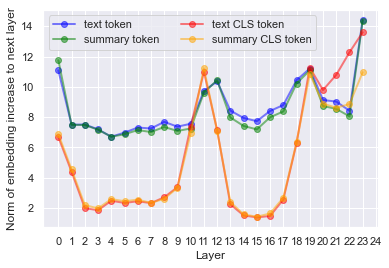
The figure shows the norm of the increment of a masked token embedding from one layer to the next. The change exactly in the middle of the transformer shows up even stronger.
A cosine between the embeddings of the same token in two neighbor layers is shown in Figure 4.

There are almost no changes in the CLS token across the layers, except the strong change in the middle layers 10-13, and then at high layers starting from layer 18. The common text tokens keep going through substantial transformation, remarkably with a stable pace - the cosign between the embeddings of neighbor layers is about 0.95, - and with much larger changes at the few special layers at which the CLS embedding also changes.
The evolution of the masked token embedding across the layers reflected in Figures 2, 3, 4 is not related to the summarization: this is how the embeddings change for a text or a summary (see also Appendix B). Looking in retrospect on the coherence in Figure 1, it seems natural to split the layers-by-layers square into four quadrants.
5 Coherence and points of similarity
5.1 Coherence
As we have seen in Figure 1, the coherence and relevance would get higher correlations with expert scores when the embeddings are picked up from different layers. The layers 18-21 for summary and around 8-11 for text would give a better correlations for coherence than in Table 1. We may speculate that the reason for this is that coherence and relevance are not as ’local’ as consistency and fluency, and need a more varied information for a judgement. When forced to use the points of similarity between the summary and the text, they do better with different layers.
In principle there should be a way to estimate the coherence and fluency of a summary without using the text, but having a text as a helpful pattern makes it easier. For better understanding of how the text helps, we can consider estimation of coherence by using the order of the points of similarity. Let us consider a correlation between the sequence of summary token locations and the sequence of the corresponding similarity locations of the tokens in the text:
| (3) |
Equation 3, with being Kendall Tau-c correlation, estimates how well the summary keeps the order of the points of similar context. Figure 5 shows correlations of this measure with expert coherence scores.

This figure is very different from the coherence part of Figure 1. For once, the diagonal - using the same layers for the summary and the text - is fine again. The plateau of high correlations is wide. Using the same layer for the summary and the text, we get correlation with coherence 0.20 or 0.21 in the layers from 7 to 15, which are quite far from the top layers. These layers, however, would be in the top part of a base BERT.
5.2 Local order of similarities
For a better insight into how the consistency is a more ’local’ quality than coherence, we will modify Kendall Tau correlation between two sequences by introducing a restriction on the distance between the elements of the first sequence. In applying such a modified Kendall correlation in Eq.3, we would consider only such pairs of summary tokens locations that are not further from each other than an (integer) interval :
| (4) |
In Eq.4 we use the modified ’local’ Kendall Tau correlation . We define as a simple Kendall Tau correlation between two sequences and , but with a restriction on the distance between the elements . As usual, , where is the number of concordant pairs, is the number of discordant pairs, and is the total number of pairs, but the counts include only the pairs for which . The concordant pair is a pair satisfying the condition , otherwise the pair is discordant. Note that in our case (Eq.4) the distance is the same no matter whether it is defined between the elements or between the ranks.
Figure 6 shows the correlations of the measure given by Eq.4 with SummEval expert scores of coherence and consistency.

We can make several simple conclusions from this figure and its underlying data:
-
1.
Consistency is a more ’local’ quality than coherence: keeping order on shorter distances provides better correlations. For consistency the layer 21 provides the best correlations - exceeding 0.18 - at the distances from 1 to 15. For coherence the layer 8 provides the best correlations - exceeding 0.22 - at the distances from 19 to 33.
-
2.
There is a wide range of layers that are helpful both for coherence and for consistency. The best layers are at the lower half of the BERT for the coherence, and close to the top for the consistency.
- 3.
6 Conclusion
In this paper we presented ESTIME-soft, Eq.2, - a variant of ESTIME applicable to more scenarios of estimating factual consistency and less sensitive to the choice of the BERT layers for the embeddings. We considered estimation of consistency as verification that the summary and the text respond the same way in all points of similar context. Each ’fact’ is represented, accordingly, as a context and a response to the context.
The context similarity for consistency and fluency has a better correlations with human scores when it uses embeddings from the BERT layers close to the top (but not at the top). For coherence the embeddings are more helpful when taken from different layers for the summary and for the text. More robust estimation of coherence is obtained by inspecting the order of the points of contextual similarity (Esq.3, 4). Embeddings from lower-middle part of BERT turned out to be the most helpful for this estimation.
A systematic comparison of evaluation measures would have to include much more measures (e.g. Fabbri et al. (2021b, a); Gabriel et al. (2021)). From our limited observations we suggest that there must be much better ways to evaluate the summary qualities, and achieve higher correlations with human scores. If currently superior correlations with human scores can be achieved by a simple measure that is based on an oversimplified representation of consistency or coherence and does not need specially tuned models or specially prepared data, then we probably should raise expectations.
References
- De Cao et al. (2020) Nicola De Cao, Michael Sejr Schlichtkrull, Wilker Aziz, and Ivan Titov. 2020. How do decisions emerge across layers in neural models? interpretation with differentiable masking. In Proceedings of the 2020 Conference on Empirical Methods in Natural Language Processing (EMNLP), pages 3243–3255, Online. Association for Computational Linguistics.
- Fabbri et al. (2021a) Alexander R. Fabbri, Wojciech Kryściński, Bryan McCann, Caiming Xiong, Richard Socher, and Dragomir Radev. 2021a. SummEval: Re-evaluating summarization evaluation. Transactions of the Association for Computational Linguistics, 9:391–409.
- Fabbri et al. (2021b) Alexander R. Fabbri, Chien-Sheng Wu, Wenhao Liu, and Caiming Xiong. 2021b. QAFactEval: Improved QA-based factual consistency evaluation for summarization. arXiv, arXiv:2112.08542.
- Falke et al. (2019) Tobias Falke, Leonardo FR Ribeiro, Prasetya Ajie Utama, Ido Dagan, and Iryna Gurevych. 2019. Ranking generated summaries by correctness: An interesting but challenging application for natural language inference. In Proceedings of the 57th Annual Meeting of the Association for Computational Linguistics, pages 2214–2220. Association for Computational Linguistics.
- Fan et al. (2018) Lisa Fan, Dong Yu, and Lu Wang. 2018. Robust neural abstractive summarization systems and evaluation against adversarial information. arXiv, arXiv:1810.06065.
- Fomicheva et al. (2021) Marina Fomicheva, Lucia Specia, and Nikolaos Aletras. 2021. Translation error detection as rationale extraction. arXiv, arXiv:2108.12197.
- Gabriel et al. (2021) Saadia Gabriel, Asli Celikyilmaz, Rahul Jha, Yejin Choi, and Jianfeng Gao. 2021. GO FIGURE: A meta evaluation of factuality in summarization. In Findings of the Association for Computational Linguistics: ACL-IJCNLP 2021, pages 478–487. Association for Computational Linguistics.
- Gao et al. (2020) Yang Gao, Wei Zhao, and Steffen Eger. 2020. SUPERT: Towards new frontiers in unsupervised evaluation metrics for multi-document summarization. In Proceedings of the 58th Annual Meeting of the Association for Computational Linguistics, pages 1347–1354. Association for Computational Linguistics.
- Geva et al. (2021) Mor Geva, Roei Schuster, Jonathan Berant, and Omer Levy. 2021. Transformer feed-forward layers are key-value memories. In Proceedings of the 2021 Conference on Empirical Methods in Natural Language Processing, pages 5484–5495, Online and Punta Cana, Dominican Republic. Association for Computational Linguistics.
- Jawahar et al. (2019) Ganesh Jawahar, Benoît Sagot, and Djamé Seddah. 2019. What does BERT learn about the structure of language? In Proceedings of the 57th Annual Meeting of the Association for Computational Linguistics, pages 3651–3657, Florence, Italy. Association for Computational Linguistics.
- Kashyap et al. (2021) Abhinav Ramesh Kashyap, Laiba Mehnaz, Bhavitvya Malik, Abdul Waheed, Devamanyu Hazarika, Min-Yen Kan, and Rajiv Ratn Shah. 2021. Analyzing the domain robustness of pretrained language models, layer by layer. In Proceedings of the Second Workshop on Domain Adaptation for NLP, pages 222–244, Kyiv, Ukraine. Association for Computational Linguistics.
- Kryscinski et al. (2020) Wojciech Kryscinski, Bryan McCann, Caiming Xiong, and Richard Socher. 2020. Evaluating the factual consistency of abstractive text summarization. In Proceedings of the 2020 Conference on Empirical Methods in Natural Language Processing, pages 9332–9346. Association for Computational Linguistics.
- Lin (2004) Chin-Yew Lin. 2004. ROUGE: A package for automatic evaluation of summaries. In Proceedings of Workshop on Text Summarization Branches Out, pages 74–81. Association for Computational Linguistics.
- Liu et al. (2019) Nelson F. Liu, Matt Gardner, Yonatan Belinkov, Matthew E. Peters, and Noah A. Smith. 2019. Linguistic knowledge and transferability of contextual representations. In Proceedings of the 2019 Conference of the North American Chapter of the Association for Computational Linguistics: Human Language Technologies, Volume 1 (Long and Short Papers), pages 1073–1094, Minneapolis, Minnesota. Association for Computational Linguistics.
- Louis and Nenkova (2009) Annie Louis and Ani Nenkova. 2009. Automatically evaluating content selection in summarization without human models. In Proceedings of the 2009 Conference on Empirical Methods in Natural Language Processing, pages 306–314. Association for Computational Linguistics.
- Maynez et al. (2020) Joshua Maynez, Shashi Narayan, Bernd Bohnet, and Ryan McDonald. 2020. On faithfulness and factuality in abstractive summarization. In Proceedings of the 58th Annual Meeting of the Association for Computational Linguistics, pages 1906–1919. Association for Computational Linguistics (2020).
- Papineni et al. (2002) Kishore Papineni, Salim Roukos, Todd Ward, and Wei-Jing Zhu. 2002. BLEU: a method for automatic evaluation of machine translation. In Proceedings of the 40th Annual Meeting of the Association for Computational Linguistics (ACL), pages 311–318, Philadelphia. Association for Computational Linguistics.
- Scialom et al. (2021) Thomas Scialom, Paul-Alexis Dray, Sylvain Lamprier, Benjamin Piwowarski, Jacopo Staiano, Alex Wang, and Patrick Gallinari. 2021. QuestEval: Summarization asks for fact-based evaluation. In Proceedings of the 2021 Conference on Empirical Methods in Natural Language Processing, pages 6594–6604. Association for Computational Linguistics.
- Scialom et al. (2019) Thomas Scialom, Sylvain Lamprier, Benjamin Piwowarski, and Jacopo Staiano. 2019. Answers unite! Unsupervised metrics for reinforced summarization models. In Proceedings of the 2019 Conference on Empirical Methods in Natural Language Processing and the 9th International Joint Conference on Natural Language Processing, pages 3246–3256, Hong Kong, China. Association for Computational Linguistics.
- Timkey and van Schijndel (2021) William Timkey and Marten van Schijndel. 2021. All bark and no bite: Rogue dimensions in transformer language models obscure representational quality. In Proceedings of the 2021 Conference on Empirical Methods in Natural Language Processing, pages 4527–4546, Online and Punta Cana, Dominican Republic. Association for Computational Linguistics.
- Turton et al. (2021) Jacob Turton, Robert Elliott Smith, and David Vinson. 2021. Deriving contextualised semantic features from BERT (and other transformer model) embeddings. In Proceedings of the 6th Workshop on Representation Learning for NLP (RepL4NLP-2021), pages 248–262.
- van Aken et al. (2019) Betty van Aken, Benjamin Winter, Alexander Löser, and Felix A. Gers. 2019. How does BERT answer questions? A layer-wise analysis of transformer representations. arXiv, arXiv:1909.04925.
- Vasilyev and Bohannon (2021a) Oleg Vasilyev and John Bohannon. 2021a. ESTIME: Estimation of summary-to-text inconsistency by mismatched embeddings. In Proceedings of the 2nd Workshop on Evaluation and Comparison of NLP Systems, pages 94–103. Association for Computational Linguistics.
- Vasilyev and Bohannon (2021b) Oleg Vasilyev and John Bohannon. 2021b. Is human scoring the best criteria for summary evaluation? In Findings of the Association for Computational Linguistics: ACL-IJCNLP 2021, pages 2184–2191. Association for Computational Linguistics.
- Vasilyev et al. (2020a) Oleg Vasilyev, Vedant Dharnidharka, and John Bohannon. 2020a. Fill in the BLANC: Human-free quality estimation of document summaries. In Proceedings of the First Workshop on Evaluation and Comparison of NLP Systems, pages 11–20. Association for Computational Linguistics.
- Vasilyev et al. (2020b) Oleg Vasilyev, Vedant Dharnidharka, Nicholas Egan, Charlene Chambliss, and John Bohannon. 2020b. Sensitivity of BLANC to human-scored qualities of text summaries. arXiv, arXiv:2010.06716.
- Voita et al. (2019) Elena Voita, Rico Sennrich, and Ivan Titov. 2019. The bottom-up evolution of representations in the transformer: A study with machine translation and language modeling objectives. In Proceedings of the 2019 Conference on Empirical Methods in Natural Language Processing and the 9th International Joint Conference on Natural Language Processing (EMNLP-IJCNLP), pages 4396–4406, Hong Kong, China. Association for Computational Linguistics.
- Wallat et al. (2020) Jonas Wallat, Jaspreet Singh, and Avishek Anand. 2020. BERTnesia: Investigating the capture and forgetting of knowledge in BERT. In Proceedings of the Third BlackboxNLP Workshop on Analyzing and Interpreting Neural Networks for NLP, pages 174–183, Online. Association for Computational Linguistics.
- Wang et al. (2020) Alex Wang, Kyunghyun Cho, and Mike Lewis. 2020. Asking and answering questions to evaluate the factual consistency of summaries. In Proceedings of the 58th Annual Meeting of the Association for Computational Linguistics, pages s 5008–5020. Association for Computational Linguistics (2020).
- Xenouleas et al. (2019) Stratos Xenouleas, Prodromos Malakasiotis, Marianna Apidianaki, and Ion Androutsopoulos. 2019. SUM-QE: a BERT-based summary quality estimation model. In Proceedings of the 2019 Conference on Empirical Methods in Natural Language Processing and the 9th International Joint Conference on Natural Language Processing, pages 6005–6011, Hong Kong, China. Association for Computational Linguistics.
- Yun et al. (2021) Zeyu Yun, Yubei Chen, Bruno Olshausen, and Yann LeCun. 2021. Transformer visualization via dictionary learning: contextualized embedding as a linear superposition of transformer factors. In Proceedings of Deep Learning Inside Out (DeeLIO): The 2nd Workshop on Knowledge Extraction and Integration for Deep Learning Architectures, pages 1–10, Online. Association for Computational Linguistics.
- Zhang et al. (2020) Tianyi Zhang, Varsha Kishore, Felix Wu, Kilian Q. Weinberger, and Yoav Artzi. 2020. BERTScore: Evaluating text generation with BERT. arXiv, arXiv:1904.09675.
Appendix A Calculation of correlations of selected measures with expert scores
Table 1 in Section 3 shows two types of rank correlations: Kendall Tau-c correlations and Spearman correlations. We do not consider non-rank correlations like Pearson because such presentations could be misleading: (1) there is a subjectivity in the intervals between the ’1-2-3-4-5’ grades in human scoring, and (2) different automated measures may be differently dilated or contracted at different intervals of their ranges - which is irrelevant for their judgements in comparing the summaries.
BLANC Vasilyev et al. (2020a) is calculated as default BLANC-help555https://github.com/PrimerAI/blanc. ESTIME and Jensen-Shannon Louis and Nenkova (2009) values are negated. SummaQA Scialom et al. (2019) is represented by SummaQA-P (prob) and SummaQA-F1 (F1 score)666https://github.com/recitalAI/summa-qa. SUPERT Gao et al. (2020) is calculated as single-doc with 20 reference sentences ’top20’777https://github.com/yg211/acl20-ref-free-eval. BLEU Papineni et al. (2002) is calculated with NLTK. BERTScore Zhang et al. (2020) (by default 888https://github.com/Tiiiger/bert_score using roberta-large) is represented by F1, precision (P) and recall (R). ROUGE Lin (2004) is calculated with rouge-score package999https://github.com/google-research/google-research/tree/master/rouge.
Appendix B Alignment of embeddings across the layers
In Section 4.2 we have seen that embeddings of the masked tokens of texts (regardless of summarization) undergo sharp changes between a few layers, - for example the change of a cosine between neighbor layer embeddings of the same token in Figure 4. If a cosine of the angle between embeddings within the same layer would make a good characterization of the layer, we would expect to observe different distributions of the cosine at the layers before and after the sharp change in Figure 4.

However, the distribution, shown in Figure 7, is more involved. Going from the input up, once the embeddings acquire the context and become on average less aligned with each other, they pass through three full periods of becoming less aligned and then more aligned again. Only the upper two dips in alignment correspond to the sharp changes in Figure 4.

Appendix C Spearman correlations: dependency on layers
In section 4.1 we supported our discussion with figures showing Kendall Tau-c correlations. Figure 8 shows the corresponding Spearman correlations. A notable difference between the figures 8 and 1 is that in the Spearman version the coherence and the relevance lost more of their level of correlations as compared to the consistency and fluency. We interpret this as a consequence of that Kendall’s (based on all pairs of observations) is more helpful than Spearman’s in accounting for overall long-range correlations. Thus, Kendall’s delivers more for coherence and relevance (as compared to the ’local’ qualities - consistency and fluency).