Conservative nonconforming virtual element method for stationary incompressible magnetohydrodynamics ^†^†thanks: .

Xiaojing Dong [email protected] Yunqing Huang [email protected] Tianwen Wang [email protected] Hunan Key Laboratory for Computation and Simulation in Science and Engineering, Key Laboratory of Intelligent Computing

\&

Information Processing of Ministry of Education, School of Mathematics and Computational Science, Xiangtan University, Xiangtan, Hunan, 411105, P.R. China

Abstract

In this paper, we propose a conservative nonconforming virtual element method for the full stationary incompressible magnetohydrodynamics model. We leverage the virtual element satisfactory divergence-free property to ensure mass conservation for the velocity field. The condition of the well-posedness of the proposed method, as well as the stability are derived. We establish optimal error estimates in the discrete energy norm for both the velocity and magnetic field. Furthermore, by employing a new technique, we obtain the optimal error estimates in $L^{2}$ -norm without any additional conditions. Finally, numerical experiments are presented to validate the theoretical analysis. In the implementation process, we adopt the effective Oseen iteration to handle the nonlinear system.

Keywords: Virtual element method; Stationary incompressible magnetohydrodynamics; error estimates; Polygonal meshes

1 Introduction

Incompressible magnetohydrodynamics (MHD) equations, coupled by multiple physical fields, model the interaction between conducting fluid and an external magnetic field. MHD equations are significant in the regions of physics and engineering, such as cooling of liquid metal in nuclear reactors, confinement for controlled thermonuclear fusion, magnetic fluid motors and the propagation of radio waves in the ionosphere [19, 15].

In the last decades, there has been a lot of research on numerical solutions of incompressible MHD equations (see [21, 19, 20, 22, 25, 18, 17, 24, 23, 31] and the references therein). Regarding handling of nonlinear terms, the classic finite element iterative methods were designed in [18, 17]. In the most mixed finite element methods, the divergence-free restriction is imposed in the weak sense and the numerical solutions violate the physical properties. The divergence-free methods have been received widely attention for incompressible MHD equations. A mixed finite element method [20] (FEM) and three interior penalty discontinuous Galerkin (DG) methods [25] for incompressible MHD were developed, with preserving exactly divergence-free velocity. Literatures [24, 23] studied structure-preserving FEMs of MHD. Moreover, a fully divergence-free FEM for MHD was proposed in [22], where the magnetic field is approximated by a magnetic vector potential.

Virtual element method (VEM), introduced with one of the simplest examples in [5, 6], is a recent technique for numerical approximation of partial differential equations and is regarded as the extension of classic FEM onto polygonal/polyhedral meshes. VEM does not require that shape functions on element are explicitly constructed, but the discrete algebraic systems can be obtained by using the degrees of freedom. An arbitrary order nonconforming virtual element was presented and applied to the Poisson equation [16] and the Stokes equations [12, 28]. The literature [8] designed an $\boldsymbol{H}^{1}$ -conforming Stokes-type virtual element $(k\geq 2)$ such that the associated discrete kernel is divergence-free. In [4, 1], the stream virtual element formulations were studied by using a suitable stream function space to approximate velocity. Piecewise divergence-free nonconforming virtual elements for Stokes problem in any dimensions were investigated in [32]. Based on the de Rham complex, the reference [35] constructed a nonconforming virtual element for Stokes problem, which is piecewise divergence-free in discrete kernel. When utilizing the virtual element proposed in [35] to solve the Navier-Stokes equations, to ensure that the constructed discrete VEM scheme achieves optimal convergence with suitable precision, the computable $L^{2}$ -projection onto the polynomials of degree $\leq k$ is required. In order to calculate $L^{2}$ -projection, the enhanced version based on the nonconforming virtual element [35] was presented in [34] for the Navier-Stokes equations. In order to derive optimal convergence with suitable precision, the enhanced version of the $H^{1}$ -conforming virtual element proposed in [5] was investigated in [2] for the reaction-diffusion problems. VEM has additionally been used to solve the resistive MHD model [3, 7].

Motivated by [3, 7], we consider a nonconforming VEM for the 2D full stationary incompressible MHD equations. Compared to the work in [3, 7], our research has two main differences: first, the model discussed here is more complex than the resistive MHD; second, the study in [3, 7] focuses on low-order virtual elements, while we develop an arbitrary order ( $k\geq 1$ ) scheme on shape-regular polygonal meshes. For keeping mass conservation, the velocity and the pressure are approximated by the enhanced nonconforming virtual element space and discontinuous piecewise polynomials. The discrete velocity is piecewise divergence-free. Each component of the magnetic field is approximated by the enhanced $H^{1}$ -conforming virtual element space. The treatment approaches for the bilinear term related to the magnetic field and the complex trilinear terms are provided. We prove the stability of the discrete formulation and establish conditions for uniqueness of the solution. Additionally, we derive optimal error estimates in the discrete energy norm and $L^{2}$ -norm for both velocity and magnetic field, as well as in the $L^{2}$ -norm for the pressure.

The rest of the paper is organized as follows. In Section 2, we briefly introduce some basis notations, the full stationary incompressible MHD equations and the weak formulation. In Section 3, we present the approximate spaces of the velocity, the magnetic field and the pressure, the virtual element discretizations of the MHD equations and the stability of the discrete formulation. In Section 4, the optimal error estimates are derived. Section 5 shows some numerical experiments to validate the theoretical analysis.

2 Preliminaries

Let $\Omega\subset\mathbb{R}^{2}$ be a bounded convex polygonal domain. We denote a two-dimensional variable by $\boldsymbol{x}$ , where $\boldsymbol{x}=(x_{1},x_{2})$ and $\boldsymbol{x}^{\perp}=(-x_{2},x_{1})$ . We use $\boldsymbol{n}$ to represent the unit outward normal vector of $\partial\Omega$ . For any polygonal subdomain $E$ of $\Omega$ , the unit outward normal vector of $\partial E$ (edge $e$ of $\partial E$ ) is denoted $\boldsymbol{n}_{E}\,(\boldsymbol{n}_{e})$ . We adopt $\mathbb{P}_{k}(\mathcal{O})$ to express the set of polynomials on $\mathcal{O}$ of degree at most $k(\geq 0)$ , here $\mathcal{O}$ can be $E$ , $\partial E$ or edge $e$ , specially $\mathbb{P}_{-2}(\mathcal{O})=\mathbb{P}_{-1}(\mathcal{O})=\{\emptyset\}$ . There exists a direct sum decomposition

\displaystyle\begin{aligned} \left[\mathbb{P}_{k}(E)\right]^{2}&=\nabla\mathbb{P}_{k+1}(E)\oplus\boldsymbol{x}^{\perp}\mathbb{P}_{k-1}(E).\end{aligned}

For scalar function $v$ and vector functions $\boldsymbol{v}=(v_{1},v_{1})$ , $\boldsymbol{w}=(w_{1},w_{2})$ , we introduce the cross product and $\mathrm{curl}$ operators

\displaystyle\begin{aligned} v\times\boldsymbol{w}&=(-w_{2}v,w_{1}v),\qquad\boldsymbol{v}\times\boldsymbol{w}=w_{2}v_{1}-w_{1}v_{2},\\ \mathrm{curl}\,v&=\left(\frac{\partial v}{\partial x_{2}},-\frac{\partial v}{\partial x_{1}}\right),\qquad\mathrm{curl}\,\boldsymbol{v}=\frac{\partial v_{2}}{\partial x_{1}}-\frac{\partial v_{1}}{\partial x_{2}}.\end{aligned}

We define some useful spaces as follows:

	$\displaystyle H^{1}(\Omega)=\left\{v\in L^{2}(\Omega):\;\nabla v\in L^{2}(\Omega)\right\},\qquad H_{0}^{1}(\Omega)=\left\{v\in H^{1}(\Omega):v\|_{\partial\Omega}=0\right\},$
	$\displaystyle\boldsymbol{H}^{1}(\Omega)=\left[H^{1}(\Omega)\right]^{2},\qquad\boldsymbol{H}_{0}^{1}(\Omega)=\left[H_{0}^{1}(\Omega)\right]^{2},\qquad\boldsymbol{L}^{2}(\Omega)=\left[L^{2}(\Omega)\right]^{2},$
	$\displaystyle\boldsymbol{H}_{n}^{1}=\left\{\boldsymbol{v}\in\boldsymbol{H}^{1}(\Omega):\boldsymbol{v}\cdot\boldsymbol{n}\|_{\partial\Omega}=0\right\},\qquad L_{0}^{2}(\Omega)=\left\{q\in L^{2}(\Omega):\;\int_{\Omega}q\,\mathrm{d}\Omega=0\right\}.$

Let $W^{k,p}(E)$ be the standard Sobolev space equipped with norm $\|\cdot\|_{k,p,E}$ and seminorm $|\cdot|_{k,p,E}$ . In particular, $W^{0,p}(E)$ is Lebesgue space with norm $\|\cdot\|_{L^{p}(E)}$ , $W^{k,2}(E)$ is Hilbertian space with norm $\|\cdot\|_{k,E}$ and seminorm $|\cdot|_{k,E}$ . $(\cdot,\cdot)_{E}$ is usual $L^{2}$ -inner product. If $E=\Omega$ , the subscript $E$ of norm, seminorm and inner product will be omitted.

We consider the two-dimensional full stationary incompressible MHD [21]:

\displaystyle\begin{cases}-R_{\nu}^{-1}\Delta\boldsymbol{u}+(\nabla\boldsymbol{u})\boldsymbol{u}+\nabla p-S_{c}\,\mathrm{curl}\,\boldsymbol{b}\times\boldsymbol{b}=\boldsymbol{f},\quad\mathrm{in}\;\Omega,\\ R_{m}^{-1}S_{c}\,\mathrm{curl}\,(\mathrm{curl}\,\boldsymbol{b})-S_{c}\,\mathrm{curl}\,(\boldsymbol{u}\times\boldsymbol{b})=\boldsymbol{g},\quad\mathrm{in}\;\Omega,\\ \mathrm{div}\,\boldsymbol{u}=0,\quad\mathrm{in}\;\Omega,\\ \mathrm{div}\,\boldsymbol{b}=0,\quad\mathrm{in}\;\Omega,\\ \boldsymbol{u}=\mathbf{0},\quad\mathrm{on}\;\partial\Omega,\\ \boldsymbol{b}\cdot\boldsymbol{n}=0,\;\boldsymbol{n}\times\mathrm{curl}\,\boldsymbol{b}=\mathbf{0},\quad\mathrm{on}\;\partial\Omega,\end{cases}

(2.1)

where $\boldsymbol{u},\,\boldsymbol{b},\,p$ are the velocity, the magnetic field and the pressure, respectively. Hydrodynamic Reynolds number $R_{\nu}$ , magnetic Reynolds number $R_{m}$ and coupling coefficient $S_{c}$ are the physical parameters of the equations. Functions $\boldsymbol{f}$ and $\boldsymbol{g}\in\boldsymbol{L}^{2}(\Omega)$ are source terms.

Like in [21], the weak formulation of problem (2.1) is as follows: $\forall(\boldsymbol{v},\boldsymbol{c},q)\in\boldsymbol{H}_{0}^{1}(\Omega)\times\boldsymbol{H}_{n}^{1}(\Omega)\times L_{0}^{2}(\Omega)$ , find $(\boldsymbol{u},\boldsymbol{b},p)\in\boldsymbol{H}_{0}^{1}(\Omega)\times\boldsymbol{H}_{n}^{1}(\Omega)\times L_{0}^{2}(\Omega)$ such that

\displaystyle\begin{cases}R_{\nu}^{-1}(\nabla\boldsymbol{u},\nabla\boldsymbol{v})+\frac{1}{2}((\nabla\boldsymbol{u})\boldsymbol{u},\boldsymbol{v})-\frac{1}{2}((\nabla\boldsymbol{v})\boldsymbol{u},\boldsymbol{u})-(\mathrm{div}\,\boldsymbol{v},p)-S_{c}\,(\mathrm{curl}\,\boldsymbol{b}\times\boldsymbol{b},\boldsymbol{v})=(\boldsymbol{f},\boldsymbol{v}),\\ R_{m}^{-1}S_{c}\,(\mathrm{curl}\,\boldsymbol{b},\mathrm{curl}\,\boldsymbol{c})+R_{m}^{-1}S_{c}\,(\mathrm{div}\,\boldsymbol{b},\mathrm{div}\,\boldsymbol{c})+S_{c}\,(\mathrm{curl}\,\boldsymbol{c}\times\boldsymbol{b},\boldsymbol{u})=(\boldsymbol{g},\boldsymbol{c}),\\ (\mathrm{div}\,\boldsymbol{u},q)=0.\end{cases}

(2.2)

According to the Proposition 3.1 in [21], we know that $\mathrm{div}\,\boldsymbol{b}=0$ can be derived from (2.2). Problem (2.2) can be rewritten as follows: find $(\boldsymbol{u},\boldsymbol{b},p)\in\boldsymbol{H}_{0}^{1}(\Omega)\times\boldsymbol{H}_{n}^{1}(\Omega)\times L_{0}^{2}(\Omega)$ such that

\displaystyle\begin{cases}A(\boldsymbol{u},\boldsymbol{b};\boldsymbol{v},\boldsymbol{c})+B(\boldsymbol{u},\boldsymbol{b};\boldsymbol{u},\boldsymbol{b};\boldsymbol{v},\boldsymbol{c})-d(\boldsymbol{v},\boldsymbol{c};p)=\left<F;\boldsymbol{v},\boldsymbol{c}\right>,\quad\forall\boldsymbol{v}\in\boldsymbol{H}_{0}^{1}(\Omega),\boldsymbol{c}\in\boldsymbol{H}_{n}^{1}(\Omega),\\ d(\boldsymbol{u},\boldsymbol{b};q)=0,\quad\forall q\in L_{0}^{2}(\Omega),\end{cases}

(2.3)

where, $\forall\boldsymbol{w}\in\boldsymbol{H}_{0}^{1}(\Omega),\boldsymbol{\psi}\in\boldsymbol{H}_{n}^{1}(\Omega)$ ,

	$\displaystyle A(\boldsymbol{u},\boldsymbol{b};\boldsymbol{v},\boldsymbol{c})=a_{0}(\boldsymbol{u},\boldsymbol{v})+a_{1}(\boldsymbol{b},\boldsymbol{c}),$
	$\displaystyle B(\boldsymbol{u},\boldsymbol{b};\boldsymbol{w},\boldsymbol{\psi};\boldsymbol{v},\boldsymbol{c})=a_{2}(\boldsymbol{\boldsymbol{u}},\boldsymbol{w},\boldsymbol{v})-a_{3}(\boldsymbol{\psi},\boldsymbol{b},\boldsymbol{v})+a_{3}(\boldsymbol{c},\boldsymbol{b},\boldsymbol{w}),\quad$
	$\displaystyle a_{0}(\boldsymbol{u},\boldsymbol{v})=R_{\nu}^{-1}(\nabla\boldsymbol{u},\nabla\boldsymbol{v}),$
	$\displaystyle a_{1}(\boldsymbol{b},\boldsymbol{c})=R_{m}^{-1}S_{c}\,(\mathrm{curl}\,\boldsymbol{b},\mathrm{curl}\,\boldsymbol{c})+R_{m}^{-1}S_{c}\,(\mathrm{div}\,\boldsymbol{b},\mathrm{div}\,\boldsymbol{c}),$
	$\displaystyle a_{2}(\boldsymbol{u},\boldsymbol{w},\boldsymbol{v})=\frac{1}{2}((\nabla\boldsymbol{w})\boldsymbol{u},\boldsymbol{v})-\frac{1}{2}((\nabla\boldsymbol{v})\boldsymbol{u},\boldsymbol{w}),$
	$\displaystyle a_{3}(\boldsymbol{\psi},\boldsymbol{b},\boldsymbol{v})=S_{c}\,(\mathrm{curl}\,\boldsymbol{\psi}\times\boldsymbol{b},\boldsymbol{v}),$
	$\displaystyle d(\boldsymbol{v},\boldsymbol{c};q)=(\mathrm{div}\,\boldsymbol{v},q),\quad\left<F;\boldsymbol{v},\boldsymbol{c}\right>=\left(\boldsymbol{f},\boldsymbol{v}\right)+(\boldsymbol{g},\boldsymbol{c}).$

For the sake of convenience, some norms are defined by

\displaystyle\|(\boldsymbol{v},\boldsymbol{c})\|_{i}=\left(\|\boldsymbol{v}\|_{i}^{2}+\|\boldsymbol{c}\|_{i}^{2}\right)^{\frac{1}{2}},\qquad\forall\boldsymbol{v},\boldsymbol{c}\in\boldsymbol{H}^{i}(\Omega),\;i=0,1,2,

and $\|F\|_{\ast}=\|(\boldsymbol{f},\boldsymbol{g})\|_{0}$ . We use the equivalent norm $\|\nabla\boldsymbol{v}\|_{0}$ to replace $\|\boldsymbol{v}\|_{1}$ for all $\boldsymbol{v}\in\boldsymbol{H}_{0}^{1}(\Omega)$ . From [14], it know that

\displaystyle\|\boldsymbol{u}\|_{L^{4}}\leq\lambda_{0}\|\boldsymbol{u}\|_{1},\qquad\|\mathrm{curl}\,\boldsymbol{b}\|_{0}^{2}+\|\mathrm{div}\,\boldsymbol{b}\|_{0}^{2}\geq\lambda_{1}\|\boldsymbol{b}\|_{1}^{2},\qquad\forall\boldsymbol{u}\in\boldsymbol{H}^{1}(\Omega),\;\boldsymbol{b}\in\boldsymbol{H}_{n}^{1}(\Omega).

(2.4)

Here and after, $\lambda_{i},i=0,1,...,5$ are positive constants independent of mesh size.

For the above linear forms, the following estimates hold (see [21]), $\forall\boldsymbol{u},\boldsymbol{w},\boldsymbol{v}\in\boldsymbol{H}_{0}^{1}(\Omega)$ , $\boldsymbol{b},\boldsymbol{\psi},\boldsymbol{c}\in\boldsymbol{H}_{n}^{1}(\Omega)$ :

$\displaystyle\|A(\boldsymbol{u},\boldsymbol{b};\boldsymbol{v},\boldsymbol{c})\|$	$\displaystyle\leq\max\left\{R_{\nu}^{-1},4R_{m}^{-1}S_{c}\right\}\\|(\boldsymbol{u},\boldsymbol{b})\\|_{1}\,\\|(\boldsymbol{v},\boldsymbol{c})\\|_{1},$	(2.5)
$\displaystyle A(\boldsymbol{u},\boldsymbol{b};\boldsymbol{u},\boldsymbol{b})$	$\displaystyle\geq\min\{R_{\nu}^{-1},\lambda_{1}R_{m}^{-1}S_{c}\}\\|(\boldsymbol{u},\boldsymbol{b})\\|_{1}^{2},$	(2.6)
$\displaystyle\|B(\boldsymbol{u},\boldsymbol{b};\boldsymbol{w},\boldsymbol{\psi};\boldsymbol{v},\boldsymbol{c})\|$	$\displaystyle\leq\sqrt[]{2}\lambda_{0}^{2}\max\{1,\sqrt[]{2}S_{c}\}\\|(\boldsymbol{u},\boldsymbol{b})\\|_{1}\,\\|(\boldsymbol{w},\boldsymbol{\psi})\\|_{1}\,\\|(\boldsymbol{v},\boldsymbol{c})\\|_{1}.$	(2.7)

The linear form $d(\cdot,\cdot;\cdot)$ is continuous and satisfies the inf-sup condition [14, 21]

\displaystyle\sup_{(\boldsymbol{v},\boldsymbol{c})\in\boldsymbol{H}_{0}^{1}(\Omega)\times\boldsymbol{H}_{n}^{1}(\Omega)}\frac{|d(\boldsymbol{v},\boldsymbol{c};q)|}{\|(\boldsymbol{v},\boldsymbol{c})\|_{1}}\geq\gamma_{0}\|q\|_{0},\qquad\forall\,q\in L_{0}^{2}(\Omega).

(2.8)

Theorem 2.1

([18]) If $\frac{\sqrt[]{2}\lambda_{0}^{2}\max\{1,\sqrt[]{2}S_{c}\}\|F\|_{\ast}}{(\min\{R_{\nu}^{-1},\lambda_{1}R_{m}^{-1}S_{c}\})^{2}}<1$ , the problem (2.3) has a unique solution $(\boldsymbol{u},\boldsymbol{b},p)\in\boldsymbol{H}_{0}^{1}(\Omega)\times\boldsymbol{H}_{n}^{1}(\Omega)\times L_{0}^{2}(\Omega)$ , satisfying

\displaystyle\min\{R_{\nu}^{-1},\lambda_{1}R_{m}^{-1}S_{c}\}\|(\boldsymbol{u},\boldsymbol{b})\|_{1}\leq\|F\|_{\ast}.

(2.9)

3 Virtual element method

3.1 Meshes and projections

Let $\{\mathcal{T}_{h}\}_{h}$ be a family of partitions of $\Omega$ into convex polygons and $h_{E}$ be diameter of element $E$ , $h$ be the largest of all diameters, $\mathcal{E}_{h}$ represent the set of edges of $\mathcal{T}_{h}$ . For each element $E$ , we have mesh regular assumptions that there exists a positive constant $\rho$ satisfying:

(A1) $E$ is star-shaped with respect to a ball $B_{E}$ of radius $\geq\rho h_{E}$ .

(A2) The distance between any two vertexes of $E$ is $\geq\rho h_{E}$ .

For an internal edge $e$ , which is a shared edge of elements $E^{+}$ and $E^{-}$ of $\mathcal{T}_{h}$ , we define the jump of $\boldsymbol{v}$ by $[\boldsymbol{v}]|_{e}=(\boldsymbol{v}|_{\partial E^{+}})|_{e}-(\boldsymbol{v}|_{\partial E^{-}})|_{e}$ , specially, for boundary edge $e$ , $[\boldsymbol{v}]|_{e}=\boldsymbol{v}|_{e}$ .

We introduce some useful projections as follows:

$H^{1}$ -seminorm projection $\Pi_{k}^{\nabla,E}$ : $\boldsymbol{H}^{1}(E)\rightarrow[\mathbb{P}_{k}(E)]^{2}$ , defined by

\displaystyle\begin{cases}\int_{E}\nabla\Pi_{k}^{\nabla,E}\boldsymbol{v}:\nabla\boldsymbol{m}_{k}\,\mathrm{d}E=\int_{E}\nabla\boldsymbol{v}:\nabla\boldsymbol{m}_{k}\,\mathrm{d}E,\qquad\forall\boldsymbol{m}_{k}\in\left[\mathbb{P}_{k}(E)\right]^{2},\;\boldsymbol{v}\in\boldsymbol{H}^{1}(E),\\ \int_{\partial E}\Pi_{k}^{\nabla,E}\boldsymbol{v}\,\mathrm{d}\partial E=\int_{\partial E}\boldsymbol{v}\;\mathrm{d}\partial E,\qquad\forall\boldsymbol{v}\in\boldsymbol{H}^{1}(E).\end{cases}

(3.1)

$L^{2}$ -projection $\Pi_{k}^{0,E}$ : $\boldsymbol{L}^{2}(E)\rightarrow\left[\mathbb{P}_{k}(E)\right]^{2}$ , defined by

\displaystyle\int_{E}\Pi_{k}^{0,E}\boldsymbol{v}\cdot\boldsymbol{m}_{k}\,\mathrm{d}E=\int_{E}\boldsymbol{v}\cdot\boldsymbol{m}_{k}\,\mathrm{d}E,\qquad\forall\boldsymbol{m}_{k}\in\left[\mathbb{P}_{k}(E)\right]^{2},\,\boldsymbol{v}\in\boldsymbol{L}^{2}(E).

(3.2)

3.2 The nonconforming element space and piecewise polynomials space

We use the enhanced nonconforming virtual element [34] to approximate the velocity. In order to describe it, we first introduce two auxiliary spaces. One space is

\displaystyle\boldsymbol{V}_{k}^{f}(E)=\left\{\boldsymbol{v}\in\boldsymbol{H}^{1}(E):\;\mathrm{div}\,\boldsymbol{v}\in\mathbb{P}_{k-1}(E),\;\mathrm{curl}\,\boldsymbol{v}\in\mathbb{P}_{k-1}(E),\;\boldsymbol{v}\cdot\boldsymbol{n}_{e}|_{e}\in\mathbb{P}_{k}(e),\;\forall e\in\partial E\right\}.

(3.3)

From [35], we know that the following direct sum decomposition holds

\displaystyle\boldsymbol{V}_{k}^{f}(E)=\boldsymbol{W}_{0}(E)\oplus\boldsymbol{W}_{1}(E),

(3.4)

where $\boldsymbol{W}_{0}(E)$ and $\boldsymbol{W}_{1}(E)$ are

\displaystyle\begin{aligned} \boldsymbol{W}_{0}(E)&=\left\{\boldsymbol{v}\in\boldsymbol{V}_{k}^{f}(E):\;\mathrm{div}\,\boldsymbol{v}=0,\;\boldsymbol{v}\cdot\boldsymbol{n}_{e}|_{e}=0,\;\forall e\in\partial E\right\},\\ \boldsymbol{W}_{1}(E)&=\left\{\boldsymbol{v}\in\boldsymbol{V}_{k}^{f}(E):\;\mathrm{curl}\,\boldsymbol{v}=0\right\}.\end{aligned}

The other space is

\displaystyle\Psi(E)=\left\{\psi\in H^{2}(E):\;\Delta^{2}\psi\in\mathbb{P}_{k-1}(E),\;\Delta\psi|_{e}\in\mathbb{P}_{k-1}(e),\;\psi|_{e}=0,\;\forall e\in\partial E\right\}.

From Lemma 3.1 in [34], it is easy to see that

\displaystyle\boldsymbol{\widetilde{V}}(E)=\boldsymbol{W}_{1}(E)\oplus\mathrm{curl}\,\Psi(E)=\boldsymbol{V}_{k}^{f}(E)+\mathrm{curl}\,\Psi(E).

(3.5)

Then, the local space is defined by

\displaystyle\begin{aligned} \boldsymbol{V}(E)=\left\{\boldsymbol{v}\in\boldsymbol{\widetilde{V}}(E):\,\int_{E}\boldsymbol{v}\cdot\boldsymbol{m}_{k}\,\mathrm{d}E=\int_{E}\Pi_{k}^{\nabla,E}\boldsymbol{v}\cdot\boldsymbol{m}_{k}\,\mathrm{d}E,\;\forall\boldsymbol{m}_{k}\in\boldsymbol{x}_{E}^{\perp}\mathbb{P}_{k-1}(E)/\boldsymbol{x}_{E}^{\perp}\mathbb{P}_{k-3}(E),\right.\\ \left.\qquad\int_{e}\boldsymbol{v}\cdot\boldsymbol{n}_{e}m_{k}\,\mathrm{d}e=\int_{e}\Pi_{k}^{\nabla,E}\boldsymbol{v}\cdot\boldsymbol{n}_{e}m_{k}\,\mathrm{d}e,\quad\forall m_{k}\in\mathbb{P}_{k}(e)/\mathbb{P}_{k-1}(e),e\subseteq\partial E\right\},\end{aligned}

(3.6)

where $\boldsymbol{x}_{E}=(\boldsymbol{x}-\boldsymbol{x}_{b})/h_{E}$ , $\boldsymbol{x}_{b}$ is the barycenter of $E$ . Obviously, $\left[\mathbb{P}_{k}(E)\right]^{2}\subseteq\boldsymbol{V}(E)$ . The degrees of freedom of $\boldsymbol{V}(E)$ are

	$\displaystyle\bullet\quad\frac{1}{\|e\|}\int_{e}\boldsymbol{v}\cdot\boldsymbol{m}_{k-1}\,\mathrm{d}e,\quad\forall\boldsymbol{m}_{k-1}\in\left[\mathbb{P}_{k-1}(e)\right]^{2},\,e\in\partial E,$		(3.7)
	$\displaystyle\bullet\quad\frac{1}{\|E\|}\int_{E}\boldsymbol{v}\cdot\boldsymbol{m}_{k-2}\,\mathrm{d}E,\quad\forall\boldsymbol{m}_{k-2}\in\left[\mathbb{P}_{k-2}(E)\right]^{2}.$		(3.8)

It is not difficult for us to find that the projection $\Pi_{k}^{\nabla,E}\circ\boldsymbol{V}(E)$ can be computed by using integration by parts and (3.7)-(3.8). According to the definition of $\boldsymbol{V}(E)$ , we know that $\mathrm{div}\,\boldsymbol{v}\in\mathbb{P}_{k-1}(E)$ for all $\boldsymbol{v}\in\boldsymbol{V}(E)$ and the expression of $\mathrm{div}\,\boldsymbol{v}$ on element $E$ can be calculated by

\displaystyle\int_{E}\mathrm{div}\,\boldsymbol{v}\cdot m_{k-1}\,\mathrm{d}E=-\int_{E}\boldsymbol{v}\cdot\nabla m_{k-1}\,\mathrm{d}E+\sum_{e\in\partial E}\int_{e}\boldsymbol{v}\cdot\boldsymbol{n}_{e}m_{k-1}\,\mathrm{d}e,\quad\forall m_{k-1}\in\mathbb{P}_{k-1}(E).

(3.9)

The first term on the right-hand side of (3.9) can be computed by (3.8). The second term is computable, since $\left(\boldsymbol{v}\cdot\boldsymbol{n}_{e}\right)|_{e}\in\mathbb{P}_{k}(e)$ and its expression can be uniquely determined by (3.6)-(3.8). For all $\boldsymbol{m}_{k}\in\left[\mathbb{P}_{k}(E)\right]^{2},\boldsymbol{v}\in\boldsymbol{V}(E)$ , there holds

\displaystyle\begin{aligned} \int_{E}\boldsymbol{v}\cdot\boldsymbol{m}_{k}\,\mathrm{d}E&=\int_{E}\boldsymbol{v}\cdot\left(\nabla m_{k+1}\oplus\boldsymbol{q}_{k}\right)\,\mathrm{d}E\\ &=-\int_{E}\mathrm{div}\,\boldsymbol{v}\cdot m_{k+1}\,\mathrm{d}E+\sum_{e\in\partial E}\int_{e}\boldsymbol{v}\cdot\boldsymbol{n}_{e}m_{k+1}\,\mathrm{d}e+\int_{E}\boldsymbol{v}\cdot\boldsymbol{q}_{k}\,\mathrm{d}E,\end{aligned}

(3.10)

where $m_{k+1}\in\mathbb{P}_{k+1}(E)$ , $\boldsymbol{q}_{k}\in\boldsymbol{x}_{E}^{\perp}\mathbb{P}_{k-1}(E)$ . Similar to the previous discussion, the right-hand side of (3.10) can be calculated by (3.7)-(3.8). Thus, the projection $\Pi_{k}^{0,E}\circ\boldsymbol{V}(E)$ is computable.

We define $L^{2}$ -projection $\Pi_{k-1}^{0,E}$ : $\nabla\boldsymbol{V}(E)\rightarrow\left[\mathbb{P}_{k-1}(E)\right]^{2\times 2}$ by

\displaystyle\int_{E}\Pi_{k-1}^{0,E}\left(\nabla\boldsymbol{v}\right):\boldsymbol{m}_{k-1}\,\mathrm{d}E=\int_{E}\nabla\boldsymbol{v}:\boldsymbol{m}_{k-1}\,\mathrm{d}E,\quad\forall\boldsymbol{m}_{k-1}\in\left[\mathbb{P}_{k-1}(E)\right]^{2\times 2}.

(3.11)

Indeed, the right-hand side of (3.11) can be calculated by integration by parts and (3.7)-(3.8). As a result, the projection $\Pi_{k-1}^{0,E}\circ(\nabla\boldsymbol{V}(E))$ is computable. With the above preparation, the global space is defined as

\displaystyle\boldsymbol{V}=\left\{\boldsymbol{v}\in\boldsymbol{L}^{2}(\Omega):\;\boldsymbol{v}|_{E}\in\boldsymbol{V}(E),\,\int_{e}[\boldsymbol{v}]\cdot\boldsymbol{m}_{k-1}\,\mathrm{d}e=0,\quad\forall\boldsymbol{m}_{k-1}\in\left[\mathbb{P}_{k-1}(e)\right]^{2},\,e\in\mathcal{E}_{h}\right\}.

(3.12)

Lemma 3.1

([34]) Let $\boldsymbol{v}\in\boldsymbol{H}^{l}(E)$ with $1\leq l\leq k+1$ , $\boldsymbol{v}_{I}$ be its degrees of freedom interpolation. Then, it holds that

\displaystyle\|\boldsymbol{v}-\boldsymbol{v}_{I}\|_{0,E}+h|\boldsymbol{v}-\boldsymbol{v}_{I}|_{1,E}\leq Ch^{l}|\boldsymbol{v}|_{l,E}.

Throughout this article, $C$ denotes a generic positive constant independent of $h$ , and might be different value at each occurrence.

As the usual framework of VEM, we define a computable local bilinear form $a_{0h}^{E}(\cdot,\cdot):\boldsymbol{V}(E)\times\boldsymbol{V}(E)\rightarrow\mathbb{R}$ by

\displaystyle a_{0h}^{E}(\boldsymbol{u}_{h},\boldsymbol{v}_{h})

\displaystyle=R_{\nu}^{-1}\Big{(}(\nabla\Pi_{k}^{\nabla,E}\boldsymbol{u}_{h},\nabla\Pi_{k}^{\nabla,E}\boldsymbol{v}_{h})_{E}+\mathrm{S}_{0}^{E}((\mathrm{I}-\Pi_{k}^{\nabla,E})\boldsymbol{u}_{h},(\mathrm{I}-\Pi_{k}^{\nabla,E})\boldsymbol{v}_{h})\Big{)},\quad\forall\boldsymbol{u}_{h},\boldsymbol{v}_{h}\in\boldsymbol{V}(E),

where $\mathrm{S}_{0}^{E}$ is a symmetric and positive definite bilinear form such that

\displaystyle\alpha_{0\ast}a_{0}^{E}(\boldsymbol{v}_{h},\boldsymbol{v}_{h})\leq R_{\nu}^{-1}\mathrm{S}_{0}^{E}(\boldsymbol{v}_{h},\boldsymbol{v}_{h})\leq\alpha_{0}^{\ast}a_{0}^{E}(\boldsymbol{v}_{h},\boldsymbol{v}_{h}),\quad\forall\boldsymbol{v}_{h}\in\boldsymbol{V}(E)\cap\mathrm{Ker}(\Pi_{k}^{\nabla,E}),

for two positive constants $\alpha_{0\ast}$ and $\alpha_{0}^{\ast}$ independent of $h$ and $E$ . The definition of $a_{0h}^{E}(\cdot,\cdot)$ and (3.1) imply

•

$k$ -consistency: for all $\boldsymbol{m}_{k}\in[\mathbb{P}_{k}(E)]^{2}$ and $\boldsymbol{v}_{h}\in\boldsymbol{V}(E)$ ,

$\displaystyle a_{0h}^{E}(\boldsymbol{m}_{k},\boldsymbol{v}_{h})=a_{0}^{E}(\boldsymbol{m}_{k},\boldsymbol{v}_{h}),$ (3.13)

•

stability: there exist two positive constants $\sigma_{0\ast}$ and $\sigma_{0}^{\ast}$ , independent of $h$ and $E$ , satisfying

\displaystyle\sigma_{0\ast}a_{0}^{E}(\boldsymbol{v}_{h},\boldsymbol{v}_{h})\leq a_{0h}^{E}(\boldsymbol{v}_{h},\boldsymbol{v}_{h})\leq\sigma_{0}^{\ast}a_{0}^{E}(\boldsymbol{v}_{h},\boldsymbol{v}_{h}),\quad\forall\boldsymbol{v}_{h}\in\boldsymbol{V}(E).

(3.14)

The pressure is approximated by discontinuous piecewise polynomials, which is defined as

\displaystyle Q=\left\{q\in L_{0}^{2}(\Omega):\,q|_{E}\in\mathbb{P}_{k-1}(E),\quad\forall\,E\in\mathcal{T}_{h}\right\}.

Let $q\in H^{l}(\Omega)\cap L_{0}^{2}(\Omega)$ , $q_{I}|_{E}$ be the $L^{2}$ -projection of $q|_{E}$ onto $\mathbb{P}_{k-1}(E)$ , then $q_{I}\in Q$ , there holds

\displaystyle\|q-q_{I}\|_{0,E}+h|q-q_{I}|_{1,E}\leq Ch^{l}|q|_{l,E},\quad\forall 1\leq l\leq k.

(3.15)

3.3 The nodal space

In order to compute the $L^{2}$ -projection onto polynomials of degree $\leq k$ , we use the enhanced $H^{1}$ -conforming virtual element [2] to approximate each component of the magnetic field. First of all, we introduce a auxiliary space

\displaystyle U_{k}^{n}(E)=\left\{c\in H^{1}(E):\,\Delta c\in\mathbb{P}_{k}(E),\,c|_{\partial E}\in C^{0}(\partial E),\,c|_{e}\in\mathbb{P}_{k}(e),\quad\forall\,e\in\partial E\right\}.

(3.16)

Then, the local enhanced space is defined as

\displaystyle\boldsymbol{M}(E)=\left\{\boldsymbol{c}\in[U_{k}^{n}(E)]^{2}:\;(\boldsymbol{c}-\Pi_{k}^{\nabla,E}\boldsymbol{c},\boldsymbol{m})_{E}=0,\quad\forall\boldsymbol{m}\in[\mathbb{P}_{k}(E)]^{2}/[\mathbb{P}_{k-2}(E)]^{2}\right\},

(3.17)

with the degrees of freedom

	$\displaystyle\bullet\quad\mathrm{the}\;\mathrm{values}\;\mathrm{of}\;\boldsymbol{c}\;\mathrm{at}\;\mathrm{vertices}\;\mathrm{of}\;E,$		(3.18)
	$\displaystyle\bullet\quad\frac{1}{\|e\|}\int_{e}\boldsymbol{c}\cdot\boldsymbol{m}_{k-2}\,\mathrm{d}e,\quad\forall\boldsymbol{m}_{k-2}\in[\mathbb{P}_{k-2}(e)]^{2},\,e\in\partial E,$		(3.19)
	$\displaystyle\bullet\quad\frac{1}{\|E\|}\int_{E}\boldsymbol{c}\cdot\boldsymbol{m}_{k-2}\,\mathrm{d}E,\quad\forall\boldsymbol{m}_{k-2}\in[\mathbb{P}_{k-2}(E)]^{2}.$		(3.20)

It is obvious that the projection $\Pi_{k}^{\nabla,E}\circ\boldsymbol{M}(E)$ can be computed by (3.18)-(3.20). From (3.20) and (3.17), we know that the projection $\Pi_{k}^{0,E}\circ\boldsymbol{M}(E)$ is computable. We define $L^{2}$ -projection $\;\Pi_{k-1}^{0,E}$ : $\mathrm{curl}\,\boldsymbol{M}(E)\rightarrow\mathbb{P}_{k-1}(E)$ by

\displaystyle\int_{E}\Pi_{k-1}^{0,E}\left(\mathrm{curl}\,\boldsymbol{c}\right)\cdot m_{k-1}\,\mathrm{d}E=\int_{E}\mathrm{curl}\,\boldsymbol{c}\cdot m_{k-1}\;\mathrm{d}E,\quad\forall m_{k-1}\in\mathbb{P}_{k-1}(E).

(3.21)

According to integration by parts and (3.18)-(3.20), it is easy to see that the projection $\Pi_{k-1}^{0,E}\circ(\mathrm{curl}\,\boldsymbol{M}(E))$ is computable. Likewise, the projection $\Pi_{k-1}^{0,E}\circ(\mathrm{div}\,\boldsymbol{M}(E))$ can be calculated.

The global space is defined as

\displaystyle\boldsymbol{M}=\left\{\boldsymbol{c}\in\boldsymbol{H}_{n}^{1}(\Omega):\;\boldsymbol{c}|_{E}\in\boldsymbol{M}(E),\quad\forall E\in\mathcal{T}_{h}\right\}.

(3.22)

Lemma 3.2

([11]) Let $\boldsymbol{c}\in\boldsymbol{H}^{l}(E)$ with $1\leq l\leq k+1$ , $\boldsymbol{c}_{I}$ be its degrees of freedom interpolation. Then, it holds that

\displaystyle\|\boldsymbol{c}-\boldsymbol{c}_{I}\|_{0,E}+h|\boldsymbol{c}-\boldsymbol{c}_{I}|_{1,E}\leq Ch^{l}|\boldsymbol{c}|_{l,E}.

We define a computable local bilinear form $a_{1h}^{E}(\cdot,\cdot):\boldsymbol{M}(E)\times\boldsymbol{M}(E)\rightarrow\mathbb{R}$ by

	$\displaystyle a_{1h}^{E}(\boldsymbol{b}_{h},\boldsymbol{c}_{h})$	$\displaystyle=R_{m}^{-1}S_{c}\left((\Pi_{k-1}^{0,E}\mathrm{curl}\,\boldsymbol{b}_{h},\Pi_{k-1}^{0,E}\mathrm{curl}\,\boldsymbol{c}_{h})_{E}+(\Pi_{k-1}^{0,E}\mathrm{div}\,\boldsymbol{b}_{h},\Pi_{k-1}^{0,E}\mathrm{div}\,\boldsymbol{c}_{h})_{E}\right.$
		$\displaystyle\left.\quad+\mathrm{S}_{1}^{E}((\mathrm{I}-\Pi_{k}^{\nabla,E})\boldsymbol{b}_{h},(\mathrm{I}-\Pi_{k}^{\nabla,E})\boldsymbol{c}_{h})\right),\quad\forall\boldsymbol{b}_{h},\boldsymbol{c}_{h}\in\boldsymbol{M}(E),$

where $\mathrm{S}_{1}^{E}$ is a symmetric and positive definite bilinear form satisfying

\displaystyle\alpha_{1\ast}\|\nabla\boldsymbol{c}_{h}\|_{0,E}\leq\mathrm{S}_{1}^{E}(\boldsymbol{c}_{h},\boldsymbol{c}_{h})\leq\alpha_{1}^{\ast}\|\nabla\boldsymbol{c}_{h}\|_{0,E},\quad\forall\boldsymbol{c}_{h}\in\boldsymbol{M}(E)\cap\mathrm{Ker}(\Pi_{k}^{\nabla,E}),

for two positive constants $\alpha_{1\ast}$ and $\alpha_{1}^{\ast}$ independent of $h$ and $E$ .

Lemma 3.3

The local bilinear form $a_{1h}^{E}(\cdot,\cdot)$ satisfies the following properties

•

$k$ -consistency: for all $\boldsymbol{m}_{k}\in[\mathbb{P}_{k}(E)]^{2}$ and $\boldsymbol{c}_{h}\in\boldsymbol{M}(E)$ ,

$\displaystyle a_{1h}^{E}(\boldsymbol{m}_{k},\boldsymbol{c}_{h})=a_{1}^{E}(\boldsymbol{m}_{k},\boldsymbol{c}_{h}),$ (3.23)

•

stability: there exist two positive constants $\sigma_{1\ast}$ and $\sigma_{1}^{\ast}$ , independent of $h$ and $E$ , such that

\displaystyle\sigma_{1\ast}a_{1}^{E}(\boldsymbol{c}_{h},\boldsymbol{c}_{h})\leq a_{1h}^{E}(\boldsymbol{c}_{h},\boldsymbol{c}_{h})\leq\sigma_{1}^{\ast}R_{m}^{-1}S_{c}\|\boldsymbol{c}_{h}\|_{1,E},\quad\forall\boldsymbol{c}_{h}\in\boldsymbol{M}(E).

(3.24)

Proof. It is clear that (3.23) holds. For the stability, we need to prove that for all $\boldsymbol{c}_{h}\in\boldsymbol{M}(E)$ ,

	$\displaystyle\\|(\mathrm{I}-\Pi_{k-1}^{0,E})\mathrm{curl}\,\boldsymbol{c}_{h}\\|_{0,E}$	$\displaystyle\leq\\|\mathrm{curl}\,(\mathrm{I}-\Pi_{k}^{\nabla,E})\boldsymbol{c}_{h}\\|_{0,E}\leq\sqrt{2}\\|\nabla(\mathrm{I}-\Pi_{k}^{\nabla,E})\boldsymbol{c}_{h}\\|_{0,E},$
	$\displaystyle\\|(\mathrm{I}-\Pi_{k-1}^{0,E})\mathrm{div}\,\boldsymbol{c}_{h}\\|_{0,E}$	$\displaystyle\leq\\|\mathrm{div}\,(\mathrm{I}-\Pi_{k}^{\nabla,E})\boldsymbol{c}_{h}\\|_{0,E}\leq\sqrt{2}\\|\nabla(\mathrm{I}-\Pi_{k}^{\nabla,E})\boldsymbol{c}_{h}\\|_{0,E},$

where $\mathrm{I}$ is an identity operator. Making use of the properties of $L^{2}$ -projection, we have

	$\displaystyle\\|(\mathrm{I}-\Pi_{k-1}^{0,E})\mathrm{curl}\,\boldsymbol{c}_{h}\\|_{0,E}^{2}$	$\displaystyle=((\mathrm{I}-\Pi_{k-1}^{0,E})\mathrm{curl}\,\boldsymbol{c}_{h},\mathrm{curl}\,(\mathrm{I}-\Pi_{k}^{\nabla,E})\boldsymbol{c}_{h})_{E}$
		$\displaystyle\leq\\|(\mathrm{I}-\Pi_{k-1}^{0,E})\mathrm{curl}\,\boldsymbol{c}_{h}\\|_{0,E}\\|\mathrm{curl}\,(\mathrm{I}-\Pi_{k}^{\nabla,E})\boldsymbol{c}_{h}\\|_{0,E},$

which is the desired result of the first inequality. Similarly, the second inequality can be derived. Thus, there hold

	$\displaystyle a_{1h}^{E}(\boldsymbol{c}_{h},\boldsymbol{c}_{h})$	$\displaystyle\leq R_{m}^{-1}S_{c}\left(\\|\Pi_{k-1}^{0,E}\mathrm{curl}\,\boldsymbol{c}_{h}\\|_{0,E}^{2}+\\|\Pi_{k-1}^{0,E}\mathrm{div}\,\boldsymbol{c}_{h}\\|_{0,E}^{2}+\alpha_{1}^{\ast}\\|\nabla(\mathrm{I}-\Pi_{k}^{\nabla,E})\boldsymbol{c}_{h}\\|_{0,E}^{2}\right)$
		$\displaystyle\leq R_{m}^{-1}S_{c}(4+\alpha_{1}^{\ast})\\|\boldsymbol{c}_{h}\\|_{1,E}^{2}=R_{m}^{-1}S_{c}\sigma_{1}^{\ast}\\|\boldsymbol{c}_{h}\\|_{1,E}^{2}$
	$\displaystyle a_{1h}^{E}(\boldsymbol{c}_{h},\boldsymbol{c}_{h})$	$\displaystyle\geq R_{m}^{-1}S_{c}\left(\\|\Pi_{k-1}^{0,E}\mathrm{curl}\,\boldsymbol{c}_{h}\\|_{0,E}^{2}+\\|\Pi_{k-1}^{0,E}\mathrm{div}\,\boldsymbol{c}_{h}\\|_{0,E}^{2}+\alpha_{1\ast}\\|\nabla(\mathrm{I}-\Pi_{k}^{\nabla,E})\boldsymbol{c}_{h}\\|_{0,E}^{2}\right)$
		$\displaystyle\geq R_{m}^{-1}S_{c}\Big{(}\\|\Pi_{k-1}^{0,E}\mathrm{curl}\,\boldsymbol{c}_{h}\\|_{0,E}^{2}+\\|\Pi_{k-1}^{0,E}\mathrm{div}\,\boldsymbol{c}_{h}\\|_{0,E}^{2}+\frac{\alpha_{1\ast}}{4}\Big{(}\\|(\mathrm{I}-\Pi_{k-1}^{0,E})\mathrm{curl}\,\boldsymbol{c}_{h}\\|_{0,E}^{2}$
		$\displaystyle\quad+\\|(\mathrm{I}-\Pi_{k-1}^{0,E})\mathrm{div}\,\boldsymbol{c}_{h}\\|_{0,E}^{2}\Big{)}\Big{)}$
		$\displaystyle\geq R_{m}^{-1}S_{c}\min\{1,\frac{\alpha_{1\ast}}{4}\}\big{(}\\|\mathrm{curl}\,\boldsymbol{c}_{h}\\|_{0,E}^{2}+\\|\mathrm{div}\,\boldsymbol{c}_{h}\\|_{0,E}^{2}\big{)}=\sigma_{1\ast}a_{1}^{E}(\boldsymbol{c}_{h},\boldsymbol{c}_{h}).$

The proof is completed. ∎

3.4 The discrete formulation

The virtual element formulation of the problem (2.3): $\forall(\boldsymbol{v}_{h},\boldsymbol{c}_{h},q_{h})\in\boldsymbol{V}\times\boldsymbol{M}\times Q$ , find $(\boldsymbol{u}_{h},\boldsymbol{b}_{h},p_{h})\in\boldsymbol{V}\times\boldsymbol{M}\times Q$ such that

\displaystyle\begin{cases}A_{h}(\boldsymbol{\boldsymbol{u}}_{h},\boldsymbol{b}_{h};\boldsymbol{v}_{h},\boldsymbol{c}_{h})+B_{h}(\boldsymbol{u}_{h},\boldsymbol{b}_{h};\boldsymbol{u}_{h},\boldsymbol{b}_{h};\boldsymbol{v}_{h},\boldsymbol{c}_{h})-d_{h}(\boldsymbol{v}_{h},\boldsymbol{c}_{h};p_{h})=\left<F_{h};\boldsymbol{v}_{h},\boldsymbol{c}_{h}\right>,\\ d_{h}(\boldsymbol{u}_{h},\boldsymbol{b}_{h};q_{h})=0,\end{cases}

(3.25)

where, $\forall\boldsymbol{w}_{h}\in\boldsymbol{V},\boldsymbol{\psi}_{h}\in\boldsymbol{M}$ ,

	$\displaystyle A_{h}(\boldsymbol{u}_{h},\boldsymbol{b}_{h};\boldsymbol{v}_{h},\boldsymbol{c}_{h})=a_{0h}(\boldsymbol{u}_{h},\boldsymbol{v}_{h})+a_{1h}(\boldsymbol{b}_{h},\boldsymbol{c}_{h})=\sum_{E\in\mathcal{T}_{h}}a_{0h}^{E}(\boldsymbol{u}_{h},\boldsymbol{v}_{h})+a_{1h}^{E}(\boldsymbol{b}_{h},\boldsymbol{c}_{h}),$
	$\displaystyle B_{h}(\boldsymbol{u}_{h},\boldsymbol{b}_{h};\boldsymbol{w}_{h},\boldsymbol{\psi}_{h};\boldsymbol{v}_{h},\boldsymbol{c}_{h})=a_{2h}(\boldsymbol{u}_{h},\boldsymbol{w}_{h},\boldsymbol{v}_{h})-a_{3h}(\boldsymbol{\psi}_{h},\boldsymbol{b}_{h},\boldsymbol{v}_{h})+a_{3h}(\boldsymbol{c}_{h},\boldsymbol{b}_{h},\boldsymbol{w}_{h}),$
	$\displaystyle a_{2h}(\boldsymbol{u}_{h},\boldsymbol{w}_{h},\boldsymbol{v}_{h})=\sum_{E\in\mathcal{T}_{h}}a_{2h}^{E}(\boldsymbol{u}_{h},\boldsymbol{w}_{h},\boldsymbol{v}_{h})$
	$\displaystyle\qquad\qquad\qquad\;\;=\sum_{E\in\mathcal{T}_{h}}\frac{1}{2}\Big{(}(\Pi_{k-1}^{0,E}(\nabla\boldsymbol{w}_{h})\Pi_{k}^{0,E}\boldsymbol{u}_{h},\Pi_{k}^{0,E}\boldsymbol{v}_{h})_{E}-(\Pi_{k-1}^{0,E}(\nabla\boldsymbol{v}_{h})\Pi_{k}^{0,E}\boldsymbol{u}_{h},\Pi_{k}^{0,E}\boldsymbol{w}_{h})_{E}\Big{)},$
	$\displaystyle a_{3h}(\boldsymbol{\psi}_{h},\boldsymbol{b}_{h},\boldsymbol{v}_{h})=\sum_{E\in\mathcal{T}_{h}}a_{3h}^{E}(\boldsymbol{\psi}_{h},\boldsymbol{b}_{h},\boldsymbol{v}_{h})=S_{c}\sum_{E\in\mathcal{T}_{h}}(\Pi_{k-1}^{0,E}\mathrm{curl}\,\boldsymbol{\psi}_{h}\times\Pi_{k}^{0,E}\boldsymbol{b}_{h},\Pi_{k}^{0,E}\boldsymbol{v}_{h})_{E},$
	$\displaystyle d_{h}(\boldsymbol{v}_{h},\boldsymbol{c}_{h};q_{h})=\sum_{E\in\mathcal{T}_{h}}d_{h}^{E}(\boldsymbol{v}_{h},\boldsymbol{c}_{h};q_{h})=\sum_{E\in\mathcal{T}_{h}}(\mathrm{div}\,\boldsymbol{v}_{h},q_{h})_{E},$
	$\displaystyle\left<F_{h};\boldsymbol{v}_{h},\boldsymbol{c}_{h}\right>=\left(\boldsymbol{f}_{h},\boldsymbol{v}_{h}\right)+(\boldsymbol{g}_{h},\boldsymbol{c}_{h})=\sum_{E\in\mathcal{T}_{h}}\left((\Pi_{k}^{0,E}\boldsymbol{f},\boldsymbol{v}_{h})_{E}+(\Pi_{k}^{0,E}\boldsymbol{g},\boldsymbol{c}_{h})_{E}\right).$

Obviously, the linear form $B_{h}(\cdot,\cdot;\cdot,\cdot;\cdot,\cdot)$ is antisymmetric, i.e.

\displaystyle B_{h}(\cdot,\cdot;\boldsymbol{w}_{h},\boldsymbol{\psi}_{h};\boldsymbol{v}_{h},\boldsymbol{c}_{h})=-B_{h}(\cdot,\cdot;\boldsymbol{v}_{h},\boldsymbol{c}_{h};\boldsymbol{w}_{h},\boldsymbol{\psi}_{h}),\quad\forall\boldsymbol{w}_{h},\boldsymbol{v}_{h}\in\boldsymbol{V},\boldsymbol{\psi}_{h},\boldsymbol{c}_{h}\in\boldsymbol{M}.

According to the definition of $\boldsymbol{V}$ , it is easy to know that $\mathrm{div}_{h}\,\boldsymbol{v}_{h}\in Q$ for any $\boldsymbol{v}_{h}\in\boldsymbol{V}$ , where $\mathrm{div}_{h}|_{E}=\mathrm{div}$ . The discrete kernel space is defined as

\displaystyle\boldsymbol{Z}_{h}=\{\boldsymbol{v}_{h}\in\boldsymbol{V}:d_{h}(\boldsymbol{v}_{h},\boldsymbol{c}_{h};q_{h})=0,\quad\forall\,q_{h}\in Q\}=\{\boldsymbol{v}_{h}\in\boldsymbol{V}:\mathrm{div}_{h}\,\boldsymbol{v}_{h}=0\}.

Due to the discrete velocity $\boldsymbol{u}_{h}\in\boldsymbol{Z}_{h}$ , then $\boldsymbol{u}_{h}$ is piecewise divergence-free. We define some norms

\displaystyle|\boldsymbol{v}_{h}|_{1,h}=\sqrt{\sum_{E\in\mathcal{T}_{h}}|\boldsymbol{v}_{h}|_{1,E}}\,,\quad\|(\boldsymbol{v}_{h},\boldsymbol{c}_{h})\|_{1,h}=\sqrt{|\boldsymbol{v}_{h}|_{1,h}^{2}+\|\boldsymbol{c}_{h}\|_{1}^{2}},\quad\forall\boldsymbol{v}_{h}\in\boldsymbol{V},\boldsymbol{c}_{h}\in\boldsymbol{M}.

There are some useful inequalities

$\displaystyle\\|\Pi_{k}^{0,E}\boldsymbol{v}_{h}\\|_{L^{4}(E)}\leq\lambda_{2}\\|\boldsymbol{v}_{h}\\|_{L^{4}(E)},$	$\displaystyle\quad\forall\boldsymbol{v}_{h}\in\boldsymbol{V},$	(3.26)
$\displaystyle\\|\boldsymbol{v}_{h}\\|_{L^{4}}\leq\lambda_{3}\|\boldsymbol{v}_{h}\|_{1,h},$	$\displaystyle\quad\forall\boldsymbol{v}_{h}\in\boldsymbol{H}_{0}^{1}(\Omega)+\boldsymbol{V},$	(3.27)
$\displaystyle\\|\boldsymbol{v}\\|_{s-1,4,E}\leq C\\|\boldsymbol{v}\\|_{s,E},$	$\displaystyle\quad\forall\boldsymbol{v}\in\boldsymbol{H}^{s}(E),$	(3.28)
$\displaystyle\\|(\mathrm{I}-\Pi_{s}^{0,E})\boldsymbol{v}\\|_{L^{4}(E)}\leq Ch_{E}^{r}\|\boldsymbol{v}\|_{r,4,E},$	$\displaystyle\quad\forall\boldsymbol{v}\in\boldsymbol{W}^{s+1,4}(E),\;0\leq r\leq s+1,$	(3.29)

where $s$ is a positive integer. By using Inverse inequality of polynomials, the properties of $L^{2}$ -projection and H $\ddot{\mathrm{o}}$ lder inequality, we obtain (3.26). The proof of (3.27), see Lemma 0.1 of Appendix in [34]. It is widely known that (3.28) holds. The inequality (3.29) can be found in [9].

Lemma 3.4

For any $\boldsymbol{u}_{h},\boldsymbol{w}_{h},\boldsymbol{v}_{h}\in\boldsymbol{V},\,\boldsymbol{b}_{h},\boldsymbol{\psi}_{h},\boldsymbol{c}_{h}\in\boldsymbol{M}$ , there hold

	$\displaystyle\|A_{h}(\boldsymbol{u}_{h},\boldsymbol{b}_{h};\boldsymbol{v}_{h},\boldsymbol{c}_{h})\|\leq\sigma^{\ast}\max\{R_{\nu}^{-1},R_{m}^{-1}S_{c}\}\\|(\boldsymbol{u}_{h},\boldsymbol{b}_{h})\\|_{1,h}\,\\|(\boldsymbol{v}_{h},\boldsymbol{c}_{h})\\|_{1,h},$		(3.30)
	$\displaystyle A_{h}(\boldsymbol{u}_{h},\boldsymbol{b}_{h};\boldsymbol{u}_{h},\boldsymbol{b}_{h})\geq\sigma_{\ast}\min\{R_{\nu}^{-1},\lambda_{1}R_{m}^{-1}S_{c}\}\\|(\boldsymbol{u}_{h},\boldsymbol{b}_{h})\\|_{1,h}^{2},$		(3.31)
	$\displaystyle\|B_{h}(\boldsymbol{u}_{h},\boldsymbol{b}_{h};\boldsymbol{w}_{h},\boldsymbol{\psi}_{h};\boldsymbol{v}_{h},\boldsymbol{c}_{h})\|\leq\hat{C}\\|(\boldsymbol{u}_{h},\boldsymbol{b}_{h})\\|_{1,h}\\|(\boldsymbol{w}_{h},\boldsymbol{\psi}_{h})\\|_{1,h}\,\\|(\boldsymbol{v}_{h},\boldsymbol{c}_{h})\\|_{1,h},$		(3.32)

where $\sigma^{\ast}=\max\{\sigma_{0}^{\ast},\sigma_{1}^{\ast}\},\sigma_{\ast}=\min\{\sigma_{0\ast},\sigma_{1\ast}\}$ , $\hat{C}$ is a constant independent of $h$ .

Proof. By Cauchy-Schwarz inequality and stabilities (3.14) and (3.24), we infer

	$\displaystyle\|A_{h}(\boldsymbol{u}_{h},\boldsymbol{b}_{h};\boldsymbol{v}_{h},\boldsymbol{c}_{h})\|$	$\displaystyle=\|a_{0h}(\boldsymbol{u}_{h},\boldsymbol{v}_{h})+a_{1h}(\boldsymbol{b}_{h},\boldsymbol{c}_{h})\|$
		$\displaystyle\leq\sum_{E\in\mathcal{T}_{h}}\left(\sigma_{0}^{\ast}R_{\nu}^{-1}\|\boldsymbol{u}_{h}\|_{1,E}\|\boldsymbol{v}_{h}\|_{1,E}+\sigma_{1}^{\ast}R_{m}^{-1}S_{c}\\|\boldsymbol{b}_{h}\\|_{1,E}\\|\boldsymbol{c}_{h}\\|_{1,E}\right)$
		$\displaystyle\leq\sigma^{\ast}\max\{R_{\nu}^{-1},R_{m}^{-1}S_{c}\}\\|(\boldsymbol{u}_{h},\boldsymbol{b}_{h})\\|_{1,h}\,\\|(\boldsymbol{v}_{h},\boldsymbol{c}_{h})\\|_{1,h}.$

Analogously, we get (3.31). Using (3.26) and (3.27) yields

$\displaystyle a_{2h}(\boldsymbol{u}_{h},\boldsymbol{w}_{h},\boldsymbol{v}_{h})$	$\displaystyle=\frac{1}{2}\sum_{E\in\mathcal{T}_{h}}\left(((\Pi_{k-1}^{0,E}\nabla\boldsymbol{w}_{h})\Pi_{k}^{0,E}\boldsymbol{u}_{h},\Pi_{k}^{0,E}\boldsymbol{v}_{h})_{E}-((\Pi_{k-1}^{0,E}\nabla\boldsymbol{v}_{h})\Pi_{k}^{0,E}\boldsymbol{u}_{h},\Pi_{k}^{0,E}\boldsymbol{w}_{h})_{E}\right)$
	$\displaystyle\leq\frac{1}{2}\lambda_{2}^{2}\sum_{E\in\mathcal{T}_{h}}\Big{(}\\|\nabla\boldsymbol{w}_{h}\\|_{0,E}\\|\boldsymbol{u}_{h}\\|_{L^{4}(E)}\\|\boldsymbol{v}_{h}\\|_{L^{4}(E)}+\\|\nabla\boldsymbol{v}_{h}\\|_{0,E}\\|\boldsymbol{u}_{h}\\|_{L^{4}(E)}\\|\boldsymbol{w}_{h}\\|_{L^{4}(E)}\Big{)}$
	$\displaystyle\leq\lambda_{2}^{2}\lambda_{3}^{2}\|\boldsymbol{u}_{h}\|_{1,h}\|\boldsymbol{w}_{h}\|_{1,h}\|\boldsymbol{v}_{h}\|_{1,h}.$	(3.33)

Similarly, we can obtain

\displaystyle a_{3h}(\boldsymbol{\psi}_{h},\boldsymbol{b}_{h},\boldsymbol{v}_{h})\leq\sqrt{2}\lambda_{0}\lambda_{2}^{2}\lambda_{3}S_{c}\|\boldsymbol{\psi}_{h}\|_{1}\|\boldsymbol{b}_{h}\|_{1}|\boldsymbol{v}_{h}|_{1,h}.

(3.34)

Combining (3.33)-(3.34), we derive (3.32). The proof is finished. ∎

Lemma 3.5

There exists a constant $\gamma_{1}>0$ independent of $h$ such that

\displaystyle\sup_{(\boldsymbol{v}_{h},\boldsymbol{c}_{h})\in\boldsymbol{V}\times\boldsymbol{M}}\frac{|d_{h}(\boldsymbol{v}_{h},\boldsymbol{c}_{h};q_{h})|}{\|(\boldsymbol{v}_{h},\boldsymbol{c}_{h})\|_{1,h}}\geq\gamma_{1}\|q_{h}\|_{0},\quad\forall q_{h}\in Q.

(3.35)

Proof. According to triangle inequality and Lemma 3.1, it is not difficult to find that $|\boldsymbol{v}_{I}|_{1,h}\leq\eta|\boldsymbol{v}|_{1}$ for all $\boldsymbol{v}\in\boldsymbol{H}_{0}^{1}(\Omega)$ , where $\eta$ is a positive constant independent of $h$ . From the definition of interpolation (see [34]) and the standard arguments in [14], for any $q_{h}\in Q$ , we have

	$\displaystyle\sup_{(\boldsymbol{v}_{I},\boldsymbol{c}_{h})\in\boldsymbol{V}\times\boldsymbol{M}}\frac{\|d_{h}(\boldsymbol{v}_{I},\boldsymbol{c}_{h};q_{h})\|}{\\|(\boldsymbol{v}_{I},\boldsymbol{c}_{h})\\|_{1,h}}$	$\displaystyle\geq\sup_{(\boldsymbol{v}_{I},\boldsymbol{c}_{h})\in\boldsymbol{V}\times\boldsymbol{0}}\frac{\|d_{h}(\boldsymbol{v}_{I},\boldsymbol{c}_{h};q_{h})\|}{\\|(\boldsymbol{v}_{I},\boldsymbol{c}_{h})\\|_{1,h}}$
		$\displaystyle=\sup_{\boldsymbol{v}_{I}\in\boldsymbol{V}}\frac{\|(\mathrm{div}\,\boldsymbol{v},q_{h})\|}{\|\boldsymbol{v}_{I}\|_{1,h}}$
		$\displaystyle\geq\frac{1}{\eta}\sup_{\boldsymbol{v}\in\boldsymbol{H}_{0}^{1}(\Omega)}\frac{\|(\mathrm{div}\,\boldsymbol{v},q_{h})\|}{\|\boldsymbol{v}\|_{1}}\geq\frac{\gamma_{0}}{\eta}\\|q_{h}\\|_{0}=\gamma_{1}\\|q_{h}\\|_{0}.$

∎

Lemma 3.6

([10]) Let $\boldsymbol{v}\in\boldsymbol{H}^{l}(E)$ , $1\leq l\leq k+1$ , there exists a polynomial $\boldsymbol{v}_{\pi}\in[\mathbb{P}_{k}(E)]^{2}$ such that

\displaystyle\|\boldsymbol{v}-\boldsymbol{v}_{\pi}\|_{L^{r}(E)}+h|\boldsymbol{v}-\boldsymbol{v}_{\pi}|_{W^{1,r}(E)}\leq Ch^{l}|\boldsymbol{v}|_{W^{l,r}(E)},\quad\forall 1\leq r\leq\infty.

Theorem 3.1

Assuming

\displaystyle\frac{\hat{C}\|F_{h}\|_{\ast}}{(\sigma_{\ast}\min\{R_{\nu}^{-1},\lambda_{1}R_{m}^{-1}S_{c}\})^{2}}<1,

(3.36)

then the problem (3.25) has a unique solution $(\boldsymbol{u}_{h},\boldsymbol{b}_{h},p_{h})\in\boldsymbol{V}\times\boldsymbol{M}\times Q$ satisfying

\displaystyle\sigma_{\ast}\min\{R_{\nu}^{-1},\lambda_{1}R_{m}^{-1}S_{c}\}\|(\boldsymbol{u}_{h},\boldsymbol{b}_{h})\|_{1,h}\leq\|F_{h}\|_{\ast}.

(3.37)

Proof. Similar to [21, 18], we can deduce (3.37) with just a few modifications. ∎

4 Error analysis

Lemma 4.1

Under assumptions (A1) and (A2), suppose $\boldsymbol{u}\in\boldsymbol{H}_{0}^{1}(\Omega)\cap\boldsymbol{H}^{k+1}(\Omega)$ , $\boldsymbol{b}\in\boldsymbol{H}_{n}^{1}(\Omega)\cap\boldsymbol{H}^{k+1}(\Omega)$ , $\boldsymbol{u}_{h}\in\boldsymbol{V}$ and $\boldsymbol{b}_{h}\in\boldsymbol{M}$ , for every $\boldsymbol{v}_{h}\in\boldsymbol{V},\boldsymbol{c}_{h}\in\boldsymbol{M}$ , there hold

	$\displaystyle\Big{\|}\sum_{E\in\mathcal{T}_{h}}a_{2}^{E}(\boldsymbol{u},\boldsymbol{u},\boldsymbol{v}_{h})-a_{2h}(\boldsymbol{u},\boldsymbol{u},\boldsymbol{v}_{h})\Big{\|}\leq Ch^{k}\\|\boldsymbol{u}\\|_{k+1}^{2}\|\boldsymbol{v}_{h}\|_{1,h},$
	$\displaystyle\Big{\|}\sum_{E\in\mathcal{T}_{h}}a_{3}^{E}(\boldsymbol{b},\boldsymbol{b},\boldsymbol{v}_{h})-a_{3h}(\boldsymbol{b},\boldsymbol{b},\boldsymbol{v}_{h})\Big{\|}\leq Ch^{k}\\|\boldsymbol{b}\\|_{k}\\|\boldsymbol{b}\\|_{k+1}\|\boldsymbol{v}_{h}\|_{1,h},$
	$\displaystyle\Big{\|}\sum_{E\in\mathcal{T}_{h}}a_{3}^{E}(\boldsymbol{c}_{h},\boldsymbol{b},\boldsymbol{u})-a_{3h}(\boldsymbol{c}_{h},\boldsymbol{b},\boldsymbol{u})\Big{\|}\leq Ch^{k}\\|\boldsymbol{b}\\|_{k+1}\\|\boldsymbol{u}\\|_{k+1}\\|\boldsymbol{c}_{h}\\|_{1},$
	$\displaystyle\big{\|}B_{h}(\boldsymbol{u},\boldsymbol{b};\boldsymbol{u},\boldsymbol{b};\boldsymbol{v}_{h},\boldsymbol{c}_{h})-B_{h}(\boldsymbol{u}_{h},\boldsymbol{b}_{h};\boldsymbol{u}_{h},\boldsymbol{b}_{h};\boldsymbol{v}_{h},\boldsymbol{c}_{h})\big{\|}\leq\hat{C}\Big{(}\\|(\boldsymbol{u}_{h},\boldsymbol{b}_{h})\\|_{1,h}\\|(\boldsymbol{v}_{h},\boldsymbol{c}_{h})\\|_{1,h}$
	$\displaystyle\qquad\qquad\qquad\quad+\\|(\boldsymbol{u}-\boldsymbol{u}_{h}+\boldsymbol{v}_{h},\boldsymbol{b}-\boldsymbol{b}_{h}+\boldsymbol{c}_{h})\\|_{1,h}\big{(}\\|(\boldsymbol{u},\boldsymbol{b})\\|_{1}+\\|(\boldsymbol{u}_{h},\boldsymbol{b}_{h})\\|_{1,h}\big{)}\Big{)}\\|(\boldsymbol{v}_{h},\boldsymbol{c}_{h})\\|_{1,h}.$

Proof. Similar to Lemma 4.3 in [9], with just a few modifications, the first inequality of Lemma 4.1 can be derived. According to the properties of $L^{2}$ -projection, H $\ddot{\mathrm{o}}$ lder inequality and (3.26)-(3.29), we have

	$\displaystyle\Big{\|}\sum_{E\in\mathcal{T}_{h}}a_{3}^{E}(\boldsymbol{b},\boldsymbol{b},\boldsymbol{v}_{h})-a_{3h}(\boldsymbol{b},\boldsymbol{b},\boldsymbol{v}_{h})\Big{\|}$
	$\displaystyle=\Big{\|}S_{c}\sum_{E\in\mathcal{T}_{h}}\int_{E}\Big{(}(\mathrm{curl}\,\boldsymbol{b}\times\boldsymbol{b})\cdot\boldsymbol{v}_{h}-(\Pi_{k-1}^{0,E}\mathrm{curl}\,\boldsymbol{b}\times\Pi_{k}^{0,E}\boldsymbol{b})\cdot\Pi_{k}^{0,E}\boldsymbol{v}_{h}\Big{)}\,\mathrm{d}E\Big{\|}$
	$\displaystyle=\Big{\|}S_{c}\sum_{E\in\mathcal{T}_{h}}\int_{E}\Big{(}\big{(}(\mathrm{I}-\Pi_{k-1}^{0,E})(\mathrm{curl}\,\boldsymbol{b}\times\boldsymbol{b})\big{)}\cdot(\mathrm{I}-\Pi_{k}^{0,E})\boldsymbol{v}_{h}+\big{(}\mathrm{curl}\,\boldsymbol{b}\times(\mathrm{I}-\Pi_{k}^{0,E})\boldsymbol{b}\big{)}\cdot\Pi_{k}^{0,E}\boldsymbol{v}_{h}$
	$\displaystyle\qquad+\big{(}(\mathrm{I}-\Pi_{k-1}^{0,E})\mathrm{curl}\,\boldsymbol{b}\times\Pi_{k}^{0,E}\boldsymbol{b}\big{)}\cdot\Pi_{k}^{0,E}\boldsymbol{v}_{h}\Big{)}\,\mathrm{d}E\Big{\|}$
	$\displaystyle\leq Ch^{k}\sum_{E\in\mathcal{T}_{h}}\big{(}\\|\mathrm{curl}\,\boldsymbol{b}\times\boldsymbol{b}\\|_{k-1,E}\|\boldsymbol{v}_{h}\|_{1,E}+\\|\boldsymbol{b}\\|_{1,E}\\|\boldsymbol{b}\\|_{k,4,E}\\|\boldsymbol{v}_{h}\\|_{L^{4}(E)}+\\|\boldsymbol{b}\\|_{k+1,E}\\|\boldsymbol{b}\\|_{L^{4}(E)}\\|\boldsymbol{v}_{h}\\|_{L^{4}(E)}\big{)}$
	$\displaystyle\leq Ch^{k}(\\|\boldsymbol{b}\\|_{1}+\\|\boldsymbol{b}\\|_{k})\\|\boldsymbol{b}\\|_{k+1}\|\boldsymbol{v}_{h}\|_{1,h}\leq Ch^{k}\\|\boldsymbol{b}\\|_{k}\\|\boldsymbol{b}\\|_{k+1}\|\boldsymbol{v}_{h}\|_{1,h}.$

Similarly, we observe that

	$\displaystyle\Big{\|}\sum_{E\in\mathcal{T}_{h}}a_{3}^{E}(\boldsymbol{c}_{h},\boldsymbol{b},\boldsymbol{u})-a_{3h}(\boldsymbol{c}_{h},\boldsymbol{b},\boldsymbol{u})\Big{\|}$
	$\displaystyle=\Big{\|}S_{c}\sum_{E\in\mathcal{T}_{h}}\int_{E}\Big{(}(\mathrm{I}-\Pi_{k-1}^{0,E})\mathrm{curl}\,\boldsymbol{c}_{h}\cdot(\mathrm{I}-\Pi_{k-1}^{0,E})(\boldsymbol{b}\times\boldsymbol{u})+\Big{(}\Pi_{k-1}^{0,E}\mathrm{curl}\,\boldsymbol{c}_{h}\times(\mathrm{I}-\Pi_{k}^{0,E})\boldsymbol{b}\Big{)}\cdot\boldsymbol{u}$
	$\displaystyle\quad+(\Pi_{k-1}^{0,E}\mathrm{curl}\,\boldsymbol{c}_{h}\times\Pi_{k}^{0,E}\boldsymbol{b})\cdot(\mathrm{I}-\Pi_{k}^{0,E})\boldsymbol{u}\Big{)}\,\mathrm{d}E\Big{\|}$
	$\displaystyle\leq Ch^{k}(\\|\boldsymbol{b}\\|_{k+1}\\|\boldsymbol{u}\\|_{k+1}+\\|\boldsymbol{b}\\|_{k+1}\\|\boldsymbol{u}\\|_{1}+\\|\boldsymbol{b}\\|_{1}\\|\boldsymbol{u}\\|_{k+1})\\|\boldsymbol{c}_{h}\\|_{1}\leq Ch^{k}\\|\boldsymbol{b}\\|_{k+1}\\|\boldsymbol{u}\\|_{k+1}\\|\boldsymbol{c}_{h}\\|_{1}.$

By the antisymmetric of the linear form $B_{h}(\cdot,\cdot;\cdot,\cdot;\cdot,\cdot)$ , we conclude that

	$\displaystyle B_{h}(\boldsymbol{u},\boldsymbol{b};\boldsymbol{u},\boldsymbol{b};\boldsymbol{v}_{h},\boldsymbol{c}_{h})-B_{h}(\boldsymbol{u}_{h},\boldsymbol{b}_{h};\boldsymbol{u}_{h},\boldsymbol{b}_{h};\boldsymbol{v}_{h},\boldsymbol{c}_{h})$
	$\displaystyle=B_{h}(\boldsymbol{u},\boldsymbol{b};\boldsymbol{u}-\boldsymbol{u}_{h},\boldsymbol{b}-\boldsymbol{b}_{h};\boldsymbol{v}_{h},\boldsymbol{c}_{h})+B_{h}(\boldsymbol{u}-\boldsymbol{u}_{h},\boldsymbol{b}-\boldsymbol{b}_{h};\boldsymbol{u}_{h},\boldsymbol{b}_{h};\boldsymbol{v}_{h},\boldsymbol{c}_{h})$
	$\displaystyle=B_{h}(\boldsymbol{u},\boldsymbol{b};\boldsymbol{u}-\boldsymbol{u}_{h}+\boldsymbol{v}_{h},\boldsymbol{b}-\boldsymbol{b}_{h}+\boldsymbol{c}_{h};\boldsymbol{v}_{h},\boldsymbol{c}_{h})$
	$\displaystyle\quad+B_{h}(\boldsymbol{u}-\boldsymbol{u}_{h}+\boldsymbol{v}_{h},\boldsymbol{b}-\boldsymbol{b}_{h}+\boldsymbol{c}_{h};\boldsymbol{u}_{h},\boldsymbol{b}_{h};\boldsymbol{v}_{h},\boldsymbol{c}_{h})-B_{h}(\boldsymbol{v}_{h},\boldsymbol{c}_{h};\boldsymbol{u}_{h},\boldsymbol{b}_{h};\boldsymbol{v}_{h},\boldsymbol{c}_{h}).$

Applying (3.32), the proof is completed. ∎

Lemma 4.2

Under assumptions (A1) and (A2), let $\boldsymbol{u}\in\boldsymbol{H}_{0}^{1}(\Omega)\cap\boldsymbol{H}^{k+1}(\Omega),\boldsymbol{w}\in\boldsymbol{H}^{2}(\Omega)$ and $p\in L_{0}^{2}(\Omega)\cap H^{k}(\Omega)$ , for every $\boldsymbol{v}_{h}\in\boldsymbol{V}$ , we can get

	$\displaystyle\|\mathcal{N}(\boldsymbol{u},p;\boldsymbol{v}_{h})\|$	$\displaystyle\leq Ch^{k}\left(R_{\nu}^{-1}\\|\boldsymbol{u}\\|_{k+1}+\\|p\\|_{k}+\\|\boldsymbol{u}\\|_{k+1}^{2}\right)\|\boldsymbol{v}_{h}\|_{1,h},$
	$\displaystyle\|\mathcal{N}(\boldsymbol{u},p;\boldsymbol{w},\boldsymbol{v}_{h})\|$	$\displaystyle\leq Ch(R_{\nu}^{-1}\\|\boldsymbol{u}\\|_{2}+\\|p\\|_{1}+\\|\boldsymbol{u}\\|_{2}\\|\boldsymbol{w}\\|_{2})\|\boldsymbol{v}_{h}\|_{1,h},$

where

	$\displaystyle\mathcal{N}(\boldsymbol{u},p;\boldsymbol{v}_{h})$	$\displaystyle=\sum_{E\in\mathcal{T}_{h}}\int_{\partial E}\left(R_{\nu}^{-1}\nabla\boldsymbol{u}\cdot\boldsymbol{n}_{E}-p\boldsymbol{n}_{E}+\frac{1}{2}(\boldsymbol{u}\cdot\boldsymbol{n}_{E})\boldsymbol{u}\right)\cdot\boldsymbol{v}_{h}\,\mathrm{d}\partial E,$
	$\displaystyle\mathcal{N}(\boldsymbol{u},p;\boldsymbol{w},\boldsymbol{v}_{h})$	$\displaystyle=\sum_{E\in\mathcal{T}_{h}}\int_{\partial E}\left(R_{\nu}^{-1}\nabla\boldsymbol{u}\cdot\boldsymbol{n}_{E}-p\boldsymbol{n}_{E}+\frac{1}{2}(\boldsymbol{w}\cdot\boldsymbol{n}_{E})\boldsymbol{u}\right)\cdot\boldsymbol{v}_{h}\,\mathrm{d}\partial E.$

For the proof of Lemma 4.2, see [27, 34].

Theorem 4.1

	$\displaystyle\\|(\boldsymbol{u}-\boldsymbol{u}_{h},\boldsymbol{b}-\boldsymbol{b}_{h})\\|_{1,h}$	$\displaystyle\leq C(\boldsymbol{u},\boldsymbol{b},p,\boldsymbol{f},\boldsymbol{g},R_{\nu},R_{m},S_{c})h^{k},$		(4.1)
	$\displaystyle\\|p-p_{h}\\|_{0}$	$\displaystyle\leq C(\boldsymbol{u},\boldsymbol{b},p,\boldsymbol{f},\boldsymbol{g},R_{\nu},R_{m},S_{c})h^{k}.$		(4.2)

Proof. According to the definition of interpolation, which implies that $\boldsymbol{u}$ and $\boldsymbol{u}_{I}$ have the same degrees of freedom, we observe that if $\boldsymbol{u}\in\boldsymbol{Z}$ , then $\boldsymbol{u}_{I}\in\boldsymbol{Z}_{h}$ . Multiplying the first and second equations in (2.1) by test functions $\delta_{\boldsymbol{u}}=\boldsymbol{u}_{h}-\boldsymbol{u}_{I}\in\boldsymbol{Z}_{h}$ and $\delta_{\boldsymbol{b}}=\boldsymbol{b}_{h}-\boldsymbol{b}_{I}\in\boldsymbol{M}$ , respectively, then using integration by parts, we deduce

\displaystyle\sum_{E\in\mathcal{T}_{h}}A^{E}(\boldsymbol{u},\boldsymbol{b};\delta_{\boldsymbol{u}},\delta_{\boldsymbol{b}})+\sum_{E\in\mathcal{T}_{h}}B^{E}(\boldsymbol{u},\boldsymbol{b};\boldsymbol{u},\boldsymbol{b};\delta_{\boldsymbol{u}},\delta_{\boldsymbol{b}})-d_{h}(\delta_{\boldsymbol{u}},\delta_{\boldsymbol{b}};p)=\left<F;\delta_{\boldsymbol{u}},\delta_{\boldsymbol{b}}\right>+\mathcal{N}(\boldsymbol{u},p;\delta_{\boldsymbol{u}}).

(4.3)

Subtracting (4.3) from (3.25), taking $\boldsymbol{v}_{h}=\delta_{\boldsymbol{u}},\boldsymbol{c}_{h}=\delta_{\boldsymbol{b}}$ and using the fact $d_{h}(\delta_{\boldsymbol{u}},\delta_{\boldsymbol{b}};p)=0$ , we derive

\displaystyle\begin{aligned} &A_{h}(\delta_{\boldsymbol{u}},\delta_{\boldsymbol{b}};\delta_{\boldsymbol{u}},\delta_{\boldsymbol{b}})\\ &=\big{\{}A_{h}(\boldsymbol{u}_{\pi}-\boldsymbol{u}_{I};\boldsymbol{b}_{\pi}-\boldsymbol{b}_{I};\delta_{\boldsymbol{u}},\delta_{\boldsymbol{b}})+\sum_{E\in\mathcal{T}_{h}}A^{E}(\boldsymbol{u}-\boldsymbol{u}_{\pi},\boldsymbol{b}-\boldsymbol{b}_{\pi};\delta_{\boldsymbol{u}},\delta_{\boldsymbol{b}})\big{\}}\\ &\quad+\big{\{}\sum_{E\in\mathcal{T}_{h}}B^{E}(\boldsymbol{u},\boldsymbol{b};\boldsymbol{u},\boldsymbol{b};\delta_{\boldsymbol{u}},\delta_{\boldsymbol{b}})-B_{h}(\boldsymbol{u},\boldsymbol{b};\boldsymbol{u},\boldsymbol{b};\delta_{\boldsymbol{u}},\delta_{\boldsymbol{b}})\big{\}}+\big{\{}B_{h}(\boldsymbol{u},\boldsymbol{b};\boldsymbol{u},\boldsymbol{b};\delta_{\boldsymbol{u}},\delta_{\boldsymbol{b}})\\ &\quad-B_{h}(\boldsymbol{u}_{h},\boldsymbol{b}_{h};\boldsymbol{u}_{h},\boldsymbol{b}_{h};\delta_{\boldsymbol{u}},\delta_{\boldsymbol{b}})\big{\}}+\big{\{}\left<F_{h};\delta_{\boldsymbol{u}},\delta_{\boldsymbol{b}}\right>-\left<F;\delta_{\boldsymbol{u}},\delta_{\boldsymbol{b}}\right>\big{\}}-\mathcal{N}(\boldsymbol{u},p;\delta_{\boldsymbol{u}})\\ &=\Theta_{1}+\Theta_{2}+\Theta_{3}+\Theta_{4}+\Theta_{5}.\end{aligned}

(4.4)

Applying triangle inequality, (3.30), Lemmas 3.1, 3.2 and 3.6, we obtain

\displaystyle\begin{aligned} \Theta_{1}&=A_{h}(\boldsymbol{u}_{\pi}-\boldsymbol{u}_{I},\boldsymbol{b}_{\pi}-\boldsymbol{b}_{I};\delta_{\boldsymbol{u}},\delta_{\boldsymbol{b}})+\sum_{E\in\mathcal{T}_{h}}A^{E}(\boldsymbol{u}-\boldsymbol{u}_{\pi},\boldsymbol{b}-\boldsymbol{b}_{\pi};\delta_{\boldsymbol{u}},\delta_{\boldsymbol{b}})\\ &\leq Ch^{k}\left(\|\boldsymbol{u}\|_{k+1}+\|\boldsymbol{b}\|_{k+1}\right)\|(\delta_{\boldsymbol{u}},\delta_{\boldsymbol{b}})\|_{1,h}.\end{aligned}

(4.5)

Using Lemma 4.1, we have

$\displaystyle\Theta_{2}$	$\displaystyle=\sum_{E\in\mathcal{T}_{h}}B^{E}(\boldsymbol{u},\boldsymbol{b};\boldsymbol{u},\boldsymbol{b};\delta_{\boldsymbol{u}},\delta_{\boldsymbol{b}})-B_{h}(\boldsymbol{u},\boldsymbol{b};\boldsymbol{u},\boldsymbol{b};\delta_{\boldsymbol{u}},\delta_{\boldsymbol{b}})$
	$\displaystyle\leq Ch^{k}\big{(}\\|\boldsymbol{u}\\|_{k+1}^{2}+\\|\boldsymbol{b}\\|_{k}\\|\boldsymbol{b}\\|_{k+1}+\\|\boldsymbol{u}\\|_{k+1}\\|\boldsymbol{b}\\|_{k+1}\big{)}\\|(\delta_{\boldsymbol{u}},\delta_{\boldsymbol{b}})\\|_{1,h},$	(4.6)
$\displaystyle\Theta_{3}$	$\displaystyle=B_{h}(\boldsymbol{u},\boldsymbol{b};\boldsymbol{u},\boldsymbol{b};\delta_{\boldsymbol{u}},\delta_{\boldsymbol{b}})-B_{h}(\boldsymbol{u}_{h},\boldsymbol{b}_{h};\boldsymbol{u}_{h},\boldsymbol{b}_{h};\delta_{\boldsymbol{u}},\delta_{\boldsymbol{b}})$
	$\displaystyle\leq\hat{C}\\|(\boldsymbol{u}_{h},\boldsymbol{b}_{h})\\|_{1,h}\\|(\delta_{\boldsymbol{u}},\delta_{\boldsymbol{b}})\\|_{1,h}^{2}+Ch^{k}\big{(}\\|\boldsymbol{u}\\|_{k+1}+\\|\boldsymbol{b}\\|_{k+1}\big{)}\big{(}\\|(\boldsymbol{u},\boldsymbol{b})\\|_{1}+\\|(\boldsymbol{u}_{h},\boldsymbol{b}_{h})\\|_{1,h}\big{)}\\|(\delta_{\boldsymbol{u}},\delta_{\boldsymbol{b}})\\|_{1,h}$
	$\displaystyle\leq\frac{\hat{C}\\|F_{h}\\|_{\ast}}{\sigma_{\ast}\min\{R_{\nu}^{-1},\lambda_{1}R_{m}^{-1}S_{c}\}}\\|(\delta_{\boldsymbol{u}},\delta_{\boldsymbol{b}})\\|_{1,h}^{2}+Ch^{k}\big{(}\\|F\\|_{\ast}+\\|F_{h}\\|_{\ast}\big{)}\big{(}\\|\boldsymbol{u}\\|_{k+1}+\\|\boldsymbol{b}\\|_{k+1}\big{)}\\|(\delta_{\boldsymbol{u}},\delta_{\boldsymbol{b}})\\|_{1,h}.$	(4.7)

From the properties of $L^{2}$ -projection, we know that

$\displaystyle\Theta_{4}$	$\displaystyle=\left<F_{h};\delta_{\boldsymbol{u}},\delta_{\boldsymbol{b}}\right>-\left<F;\delta_{\boldsymbol{u}},\delta_{\boldsymbol{b}}\right>$
	$\displaystyle=\sum_{E\in\mathcal{T}_{h}}\int_{E}(\boldsymbol{f}-\Pi_{k}^{0,E}\boldsymbol{f})\cdot(\mathrm{I}-\Pi_{0}^{0,E})\delta_{\boldsymbol{u}}+(\boldsymbol{g}-\Pi_{k}^{0,E}\boldsymbol{g})\cdot(\mathrm{I}-\Pi_{0}^{0,E})\delta_{\boldsymbol{b}}\,\,\mathrm{d}E$
	$\displaystyle\leq C\sum_{E\in\mathcal{T}_{h}}\big{(}h_{E}^{k}\|\boldsymbol{f}\|_{k-1,E}\|\delta_{\boldsymbol{u}}\|_{1,E}+h_{E}^{k}\|\boldsymbol{g}\|_{k-1,E}\|\delta_{\boldsymbol{b}}\|_{1,E}\big{)}$
	$\displaystyle\leq Ch^{k}\big{(}\\|\boldsymbol{f}\\|_{k-1}+\\|\boldsymbol{g}\\|_{k-1}\big{)}\\|(\delta_{\boldsymbol{u}},\delta_{\boldsymbol{b}})\\|_{1,h}.$	(4.8)

Applying Lemma 4.2, it is easy to see that

\displaystyle\Theta_{5}=-\mathcal{N}(\boldsymbol{u},p;\delta_{\boldsymbol{u}})\leq Ch^{k}\big{(}\|\boldsymbol{u}\|_{k+1}+\|p\|_{k}+\|\boldsymbol{u}\|_{k+1}^{2}\big{)}\|(\delta_{\boldsymbol{u}},\delta_{\boldsymbol{b}})\|_{1,h}.

(4.9)

Substituting (4.5)-(4.9) into (4.4) and using (3.31), we infer

	$\displaystyle\sigma_{\ast}\min\{R_{\nu}^{-1},\lambda_{1}R_{m}^{-1}S_{c}\}\Big{(}1-\frac{\hat{C}\\|F_{h}\\|_{\ast}}{(\sigma_{\ast}\min\{R_{\nu}^{-1},\lambda_{1}R_{m}^{-1}S_{c}\})^{2}}\Big{)}\\|(\delta_{\boldsymbol{u}},\delta_{\boldsymbol{b}})\\|_{1,h}$
	$\displaystyle\leq C(\boldsymbol{u},\boldsymbol{b},p,\boldsymbol{f},\boldsymbol{g},R_{\nu},R_{m},S_{c})h^{k}.$		(4.10)

By (4.10), assumption (3.36) and triangle inequality, we can derive (4.1).

Substacting (4.3) from (3.25), taking $\delta_{\boldsymbol{u}}=\boldsymbol{v}_{h},\delta_{\boldsymbol{b}}=\boldsymbol{c}_{h}$ , we obtain

\displaystyle\begin{aligned} &d_{h}(\boldsymbol{v}_{h},\boldsymbol{c}_{h};p)-d_{h}(\boldsymbol{v}_{h},\boldsymbol{c}_{h};p_{h})\\ &=\Big{\{}\sum_{E\in\mathcal{T}_{h}}A^{E}(\boldsymbol{u}-\boldsymbol{u}_{\pi},\boldsymbol{b}-\boldsymbol{b}_{\pi};\boldsymbol{v}_{h},\boldsymbol{c}_{h})-A_{h}(\boldsymbol{u}_{h}-\boldsymbol{u}_{\pi},\boldsymbol{b}_{h}-\boldsymbol{b}_{\pi};\boldsymbol{v}_{h},\boldsymbol{c}_{h})\Big{\}}\\ &\quad+\Big{\{}\sum_{E\in\mathcal{T}_{h}}B^{E}(\boldsymbol{u},\boldsymbol{b};\boldsymbol{u},\boldsymbol{b};\boldsymbol{v}_{h},\boldsymbol{c}_{h})-B_{h}(\boldsymbol{u},\boldsymbol{b};\boldsymbol{u},\boldsymbol{b};\boldsymbol{v}_{h},\boldsymbol{c}_{h})\Big{\}}+\big{\{}B_{h}(\boldsymbol{u},\boldsymbol{b};\boldsymbol{u},\boldsymbol{b};\boldsymbol{v}_{h},\boldsymbol{c}_{h})\\ &\quad-B_{h}(\boldsymbol{u}_{h},\boldsymbol{b}_{h};\boldsymbol{u}_{h},\boldsymbol{b}_{h};\boldsymbol{v}_{h},\boldsymbol{c}_{h})\big{\}}+\big{\{}\left<F_{h};\boldsymbol{v}_{h},\boldsymbol{c}_{h}\right>-\left<F;\boldsymbol{v}_{h},\boldsymbol{c}_{h}\right>\big{\}}-\mathcal{N}(\boldsymbol{u},p;\boldsymbol{v}_{h})\\ &=\overline{\Theta}_{1}+\overline{\Theta}_{2}+\overline{\Theta}_{3}+\overline{\Theta}_{4}+\overline{\Theta}_{5}.\end{aligned}

(4.11)

Similar to the estimates of the terms $\Theta_{1},\Theta_{2},\Theta_{4},\Theta_{5}$ , there hold

$\displaystyle\overline{\Theta}_{1}$	$\displaystyle\leq C\Big{(}\\|(\boldsymbol{u}-\boldsymbol{u}_{h},\boldsymbol{b}-\boldsymbol{b}_{h})\\|_{1,h}+h^{k}\big{(}\\|\boldsymbol{u}\\|_{k+1}+\\|\boldsymbol{b}\\|_{k+1}\big{)}\Big{)}\\|(\boldsymbol{v}_{h},\boldsymbol{c}_{h})\\|_{1,h},$	(4.12)
$\displaystyle\overline{\Theta}_{2}$	$\displaystyle\leq Ch^{k}\Big{(}\\|\boldsymbol{u}\\|_{k+1}^{2}+\\|\boldsymbol{b}\\|_{k}\\|\boldsymbol{b}\\|_{k+1}+\\|\boldsymbol{u}\\|_{k+1}\\|\boldsymbol{b}\\|_{k+1}\Big{)}\\|(\boldsymbol{v}_{h},\boldsymbol{c}_{h})\\|_{1,h},$	(4.13)
$\displaystyle\overline{\Theta}_{4}$	$\displaystyle\leq Ch^{k}\big{(}\\|\boldsymbol{f}\\|_{k-1}+\\|\boldsymbol{g}\\|_{k-1}\big{)}\\|(\boldsymbol{v}_{h},\boldsymbol{c}_{h})\\|_{1,h},$	(4.14)
$\displaystyle\overline{\Theta}_{5}$	$\displaystyle\leq Ch^{k}\big{(}\\|\boldsymbol{u}\\|_{k+1}+\\|p\\|_{k}+\\|\boldsymbol{u}\\|_{k+1}^{2}\big{)}\\|(\boldsymbol{v}_{h},\boldsymbol{c}_{h})\\|_{1,h}.$	(4.15)

For the estimate of the term $\overline{\Theta}_{3}$ , we observe that

\displaystyle\begin{aligned} \overline{\Theta}_{3}&=B_{h}(\boldsymbol{u},\boldsymbol{b};\boldsymbol{u},\boldsymbol{b};\boldsymbol{v}_{h},\boldsymbol{c}_{h})-B_{h}(\boldsymbol{u}_{h},\boldsymbol{b}_{h};\boldsymbol{u}_{h},\boldsymbol{b}_{h};\boldsymbol{v}_{h},\boldsymbol{c}_{h})\\ &=B_{h}(\boldsymbol{u}-\boldsymbol{u}_{h},\boldsymbol{b}-\boldsymbol{b}_{h};\boldsymbol{u},\boldsymbol{b};\boldsymbol{v}_{h},\boldsymbol{c}_{h})+B_{h}(\boldsymbol{u}_{h},\boldsymbol{b}_{h};\boldsymbol{u}-\boldsymbol{u}_{h},\boldsymbol{b}-\boldsymbol{b}_{h};\boldsymbol{v}_{h},\boldsymbol{c}_{h})\\ &\leq C\|(\boldsymbol{u}-\boldsymbol{u}_{h},\boldsymbol{b}-\boldsymbol{b}_{h})\|_{1,h}\Big{(}\|(\boldsymbol{u}_{h},\boldsymbol{b}_{h})\|_{1,h}+\|(\boldsymbol{u},\boldsymbol{b})\|_{1}\Big{)}\|(\boldsymbol{v}_{h},\boldsymbol{c}_{h})\|_{1,h}.\end{aligned}

(4.16)

Combining (4.12)-(4.16) and using (4.1), we conclude that

\displaystyle|d_{h}(\boldsymbol{v}_{h},\boldsymbol{c}_{h};p_{h})-d_{h}(\boldsymbol{v}_{h},\boldsymbol{c}_{h};p)|\leq C(\boldsymbol{u},\boldsymbol{b},p,\boldsymbol{f},\boldsymbol{g},R_{\nu},R_{m},S_{c})h^{k}\|(\boldsymbol{v}_{h},\boldsymbol{c}_{h})\|_{1,h}.

(4.17)

Applying the discrete inf-sup condition (3.35) yields

	$\displaystyle\\|p_{h}-p_{I}\\|_{0}$	$\displaystyle\leq\frac{1}{\gamma_{1}}\sup_{(\boldsymbol{v}_{h},\boldsymbol{c}_{h})\in\boldsymbol{V}\times\boldsymbol{M}}\frac{\|d_{h}(\boldsymbol{v}_{h},\boldsymbol{c}_{h};p_{h}-p_{I})\|}{\\|(\boldsymbol{v}_{h},\boldsymbol{c}_{h})\\|_{1,h}}$
		$\displaystyle=\frac{1}{\gamma_{1}}\sup_{(\boldsymbol{v}_{h},\boldsymbol{c}_{h})\in\boldsymbol{V}\times\boldsymbol{M}}\frac{\|d_{h}(\boldsymbol{v}_{h},\boldsymbol{c}_{h};p_{h}-p)\|}{\\|(\boldsymbol{v}_{h},\boldsymbol{c}_{h})\\|_{1,h}},$

which implies

\displaystyle\|p_{h}-p_{I}\|_{0}

\displaystyle\leq C(\boldsymbol{u},\boldsymbol{b},p,\boldsymbol{f},\boldsymbol{g},R_{\nu},R_{m},S_{c})h^{k}.

By triangle inequality and (3.15), we get (4.2). The proof is completed. ∎

For $L^{2}$ -norm of error, we consider the following dual problem, see [21, 26].

\displaystyle\begin{cases}-R_{\nu}^{-1}\Delta\boldsymbol{w}+\displaystyle\frac{1}{2}\left((\nabla\boldsymbol{u})^{\mathrm{T}}\boldsymbol{w}-(\nabla\boldsymbol{w})^{\mathrm{T}}\boldsymbol{u}\right)-(\nabla\boldsymbol{w})\boldsymbol{u}+\nabla s+S_{c}\mathrm{curl}\,\boldsymbol{\Phi}\times\boldsymbol{b}=\boldsymbol{u}-\boldsymbol{u}_{h},\quad\mathrm{in}\;\Omega,\\ R_{m}^{-1}S_{c}\left(\mathrm{curl}\,\mathrm{curl}\,\boldsymbol{\Phi}-\nabla(\mathrm{div}\,\boldsymbol{\Phi})\right)+S_{c}\left(\mathrm{curl}\,\boldsymbol{b}\times\boldsymbol{w}-\mathrm{curl}\,\boldsymbol{\Phi}\times\boldsymbol{u}-\mathrm{curl}(\boldsymbol{b}\times\boldsymbol{w})\right)=\boldsymbol{b}-\boldsymbol{b}_{h},\quad\mathrm{in}\;\Omega,\\ \mathrm{div}\,\boldsymbol{w}=0,\quad\mathrm{in}\;\Omega,\\ \boldsymbol{w}=0,\quad\boldsymbol{b}\cdot\boldsymbol{n}=0,\quad\mathrm{curl}\,\boldsymbol{\Phi}\times\boldsymbol{n}=0,\quad\mathrm{on}\;\partial\Omega,\end{cases}

(4.18)

where $(\cdot)^{\mathrm{T}}$ represents the normal transpose. We assume that the solution of (4.18) satisfies $(\boldsymbol{w},\boldsymbol{\Phi},s)\in\boldsymbol{H}^{2}(\Omega)\times\boldsymbol{H}^{2}(\Omega)\times H^{1}(\Omega)$ and there exists a constant $\lambda_{4}$ such that

\displaystyle\|(\boldsymbol{w},\boldsymbol{\Phi})\|_{2}+\|s\|_{1}\leq\lambda_{4}\|(\boldsymbol{u}-\boldsymbol{u}_{h},\boldsymbol{b}-\boldsymbol{b}_{h})\|_{0}.

(4.19)

Theorem 4.2

Under assumptions (A1), (A2) and (3.36), let $(\boldsymbol{u},\boldsymbol{b},p)\in(\boldsymbol{H}_{0}^{1}(\Omega)\cap\boldsymbol{H}^{k+1}(\Omega))\times(\boldsymbol{H}_{n}^{1}(\Omega)\cap\boldsymbol{H}^{k+1}(\Omega))\times(L_{0}^{2}(\Omega)\cap H^{k}(\Omega))$ and $(\boldsymbol{u}_{h},\boldsymbol{b}_{h},p_{h})\in\boldsymbol{V}\times\boldsymbol{M}\times Q$ be the solutions of (2.3) and (3.25), respectively. If $(\boldsymbol{w},\boldsymbol{\Phi},s)\in(\boldsymbol{H}^{2}(\Omega)\cap\boldsymbol{H}_{0}^{1}(\Omega))\times(\boldsymbol{H}^{2}(\Omega)\cap\boldsymbol{H}_{n}^{1}(\Omega))\times(H^{1}(\Omega)\cap L_{0}^{2}(\Omega))$ , there holds

\displaystyle\|(\boldsymbol{u}-\boldsymbol{u}_{h},\boldsymbol{b}-\boldsymbol{b}_{h})\|_{0}

\displaystyle\leq C(\boldsymbol{u},\boldsymbol{b},p,\boldsymbol{f},\boldsymbol{g},R_{\nu},R_{m},S_{c})h^{k+1}.

Proof. Multiplying (4.18) by test functions $\boldsymbol{u}-\boldsymbol{u}_{h}$ and $\boldsymbol{b}-\boldsymbol{b}_{h}$ , then adding (3.25) and substracting (4.3), with $\boldsymbol{v}_{h}=\delta_{\boldsymbol{u}}=\boldsymbol{w}_{I}\in\boldsymbol{Z}_{h},\boldsymbol{c}_{h}=\delta_{\boldsymbol{b}}=\boldsymbol{\Phi}_{I}$ , we deduce

	$\displaystyle\\|(\boldsymbol{u}-\boldsymbol{u}_{h},\boldsymbol{b}-\boldsymbol{b}_{h})\\|_{0}^{2}$
	$\displaystyle=\sum_{E\in\mathcal{T}_{h}}A^{E}(\boldsymbol{u}-\boldsymbol{u}_{h},\boldsymbol{b}-\boldsymbol{b}_{h};\boldsymbol{w},\boldsymbol{\Phi})+\sum_{E\in\mathcal{T}_{h}}B^{E}(\boldsymbol{u},\boldsymbol{b};\boldsymbol{u}-\boldsymbol{u}_{h},\boldsymbol{b}-\boldsymbol{b}_{h};\boldsymbol{w},\boldsymbol{\Phi})$
	$\displaystyle\quad+\sum_{E\in\mathcal{T}_{h}}B^{E}(\boldsymbol{u}-\boldsymbol{u}_{h},\boldsymbol{b}-\boldsymbol{b}_{h};\boldsymbol{u},\boldsymbol{b};\boldsymbol{w},\boldsymbol{\Phi})-\mathcal{N}(\boldsymbol{w},s;\boldsymbol{u},\boldsymbol{u}-\boldsymbol{u}_{h})+A_{h}(\boldsymbol{u}_{h},\boldsymbol{b}_{h};\boldsymbol{w}_{I},\boldsymbol{\Phi}_{I})$
	$\displaystyle\quad+B_{h}(\boldsymbol{u}_{h},\boldsymbol{b}_{h};\boldsymbol{u}_{h},\boldsymbol{b}_{h};\boldsymbol{w}_{I},\boldsymbol{\Phi}_{I})-\left<F_{h};\boldsymbol{w}_{I},\boldsymbol{\Phi}_{I}\right>-\sum_{E\in\mathcal{T}_{h}}A^{E}(\boldsymbol{u},\boldsymbol{b};\boldsymbol{w}_{I},\boldsymbol{\Phi}_{I})$
	$\displaystyle\quad-\sum_{E\in\mathcal{T}_{h}}B^{E}(\boldsymbol{u},\boldsymbol{b};\boldsymbol{u},\boldsymbol{b};\boldsymbol{w}_{I},\boldsymbol{\Phi}_{I})+\left<F;\boldsymbol{w}_{I},\boldsymbol{\Phi}_{I}\right>+\mathcal{N}(\boldsymbol{u},p;\boldsymbol{w}_{I})$
	$\displaystyle=\sum_{E\in\mathcal{T}_{h}}A^{E}(\boldsymbol{u}-\boldsymbol{u}_{h},\boldsymbol{b}-\boldsymbol{b}_{h};\boldsymbol{w}-\boldsymbol{w}_{I},\boldsymbol{\Phi}-\boldsymbol{\Phi}_{I})+\Big{\{}A_{h}(\boldsymbol{u}_{h},\boldsymbol{b}_{h};\boldsymbol{w}_{I},\boldsymbol{\Phi}_{I})-\sum_{E\in\mathcal{T}_{h}}A^{E}(\boldsymbol{u}_{h},\boldsymbol{b}_{h};\boldsymbol{w}_{I},\boldsymbol{\Phi}_{I})\Big{\}}$
	$\displaystyle\quad+\Big{\{}B_{h}(\boldsymbol{u}_{h},\boldsymbol{b}_{h};\boldsymbol{u}_{h},\boldsymbol{b}_{h};\boldsymbol{w}_{I}-\boldsymbol{w},\boldsymbol{\Phi}_{I}-\boldsymbol{\Phi})-\sum_{E\in\mathcal{T}_{h}}B^{E}(\boldsymbol{u},\boldsymbol{b};\boldsymbol{u},\boldsymbol{b};\boldsymbol{w}_{I}-\boldsymbol{w},\boldsymbol{\Phi}_{I}-\boldsymbol{\Phi})\Big{\}}$
	$\displaystyle\quad+\sum_{E\in\mathcal{T}_{h}}B^{E}(\boldsymbol{u}-\boldsymbol{u}_{h},\boldsymbol{b}-\boldsymbol{b}_{h};\boldsymbol{u}-\boldsymbol{u}_{h},\boldsymbol{b}-\boldsymbol{b}_{h};\boldsymbol{w},\boldsymbol{\Phi})-\Big{\{}\sum_{E\mathcal{T}_{h}}B^{E}(\boldsymbol{u}_{h},\boldsymbol{b}_{h};\boldsymbol{u}_{h},\boldsymbol{b}_{h};\boldsymbol{w},\boldsymbol{\Phi})$
	$\displaystyle\quad-B_{h}(\boldsymbol{u}_{h},\boldsymbol{b}_{h};\boldsymbol{u}_{h},\boldsymbol{b}_{h};\boldsymbol{w},\boldsymbol{\Phi})\Big{\}}+\left<F-F_{h};\boldsymbol{w}_{I},\boldsymbol{\Phi}_{I}\right>+\big{\{}\mathcal{N}(\boldsymbol{u},p;\boldsymbol{w}_{I}-\boldsymbol{w})$
	$\displaystyle\quad-\mathcal{N}(\boldsymbol{w},s;\boldsymbol{u},\boldsymbol{u}-\boldsymbol{u}_{h})\big{\}}$
	$\displaystyle=\Gamma_{1}+\Gamma_{2}+\Gamma_{3}+\Gamma_{4}+\Gamma_{5}+\Gamma_{6}+\Gamma_{7},$		(4.20)

where $\mathcal{N}(\boldsymbol{u},p;\boldsymbol{w})=0$ . Applying Lemmas 3.1-3.2 and (4.19), we get

\displaystyle\Gamma_{1}\leq Ch\|(\boldsymbol{u}-\boldsymbol{u}_{h},\boldsymbol{b}-\boldsymbol{b}_{h})\|_{1,h}\|(\boldsymbol{u}-\boldsymbol{u}_{h},\boldsymbol{b}-\boldsymbol{b}_{h})\|_{0}.

(4.21)

Making use of consistencies (3.13), (3.23), triangle inequality and (4.19), we obtain

$\displaystyle\Gamma_{2}$	$\displaystyle=A_{h}(\boldsymbol{u}_{h},\boldsymbol{b}_{h};\boldsymbol{w}_{I},\boldsymbol{\Phi}_{I})-\sum_{E\in\mathcal{T}_{h}}A^{E}(\boldsymbol{u}_{h},\boldsymbol{b}_{h};\boldsymbol{w}_{I},\boldsymbol{\Phi}_{I})$
	$\displaystyle=A_{h}(\boldsymbol{u}_{h}-\boldsymbol{u}_{\pi},\boldsymbol{b}_{h}-\boldsymbol{b}_{\pi};\boldsymbol{w}_{I}-\boldsymbol{w}_{\pi},\boldsymbol{\Phi}_{I}-\boldsymbol{\Phi}_{\pi})-\sum_{E\in\mathcal{T}_{h}}A^{E}(\boldsymbol{u}_{h}-\boldsymbol{u}_{\pi},\boldsymbol{b}_{h}-\boldsymbol{b}_{\pi};\boldsymbol{w}_{I}-\boldsymbol{w}_{\pi},\boldsymbol{\Phi}_{I}-\boldsymbol{\Phi}_{\pi})$
	$\displaystyle\leq C\\|(\boldsymbol{u}_{h}-\boldsymbol{u}_{\pi},\boldsymbol{b}_{h}-\boldsymbol{b}_{\pi})\\|_{1,h}\\|(\boldsymbol{w}_{I}-\boldsymbol{w}_{\pi},\boldsymbol{\Phi}_{I}-\boldsymbol{\Phi}_{\pi})\\|_{1,h}$
	$\displaystyle\leq C\Big{(}h\\|(\boldsymbol{u}-\boldsymbol{u}_{h},\boldsymbol{b}-\boldsymbol{b}_{h})\\|_{1,h}+h^{k+1}\big{(}\\|\boldsymbol{u}\\|_{k+1}+\\|\boldsymbol{b}\\|_{k+1}\big{)}\Big{)}\\|(\boldsymbol{u}-\boldsymbol{u}_{h},\boldsymbol{b}-\boldsymbol{b}_{h})\\|_{0}.$	(4.22)

From Lemmas 3.4, 4.1, 3.1, 3.2 and (4.19), we observe that

$\displaystyle\Gamma_{3}$	$\displaystyle=B_{h}(\boldsymbol{u}_{h},\boldsymbol{b}_{h};\boldsymbol{u}_{h},\boldsymbol{b}_{h};\boldsymbol{w}_{I}-\boldsymbol{w},\boldsymbol{\Phi}_{I}-\boldsymbol{\Phi})-\sum_{E\in\mathcal{T}_{h}}B^{E}(\boldsymbol{u},\boldsymbol{b};\boldsymbol{u},\boldsymbol{b};\boldsymbol{w}_{I}-\boldsymbol{w},\boldsymbol{\Phi}_{I}-\boldsymbol{\Phi})$
	$\displaystyle=B_{h}(\boldsymbol{u}_{h}-\boldsymbol{u},\boldsymbol{b}_{h}-\boldsymbol{b};\boldsymbol{u}_{h},\boldsymbol{b}_{h};\boldsymbol{w}_{I}-\boldsymbol{w},\boldsymbol{\Phi}_{I}-\boldsymbol{\Phi})+B_{h}(\boldsymbol{u},\boldsymbol{b};\boldsymbol{u}_{h}-\boldsymbol{u},\boldsymbol{b}_{h}-\boldsymbol{b};\boldsymbol{w}_{I}-\boldsymbol{w},\boldsymbol{\Phi}_{I}-\boldsymbol{\Phi})$
	$\displaystyle\quad+B_{h}(\boldsymbol{u},\boldsymbol{b};\boldsymbol{u},\boldsymbol{b};\boldsymbol{w}_{I}-\boldsymbol{w},\boldsymbol{\Phi}_{I}-\boldsymbol{\Phi})-\sum_{E\in\mathcal{T}_{h}}B^{E}(\boldsymbol{u},\boldsymbol{b};\boldsymbol{u},\boldsymbol{b};\boldsymbol{w}-\boldsymbol{w}_{I},\boldsymbol{\Phi}_{I}-\boldsymbol{\Phi})$
	$\displaystyle\leq Ch\big{(}\\|(\boldsymbol{u},\boldsymbol{b})\\|_{1}+\\|(\boldsymbol{u}_{h},\boldsymbol{b}_{h})\\|_{1,h}\big{)}\\|(\boldsymbol{u}-\boldsymbol{u}_{h},\boldsymbol{b}-\boldsymbol{b}_{h})\\|_{1,h}\\|(\boldsymbol{u}-\boldsymbol{u}_{h},\boldsymbol{b}-\boldsymbol{b}_{h})\\|_{0}$
	$\displaystyle\quad+Ch^{k+1}\big{(}\\|\boldsymbol{u}\\|_{k+1}^{2}+\\|\boldsymbol{b}\\|_{k}\\|\boldsymbol{b}\\|_{k+1}+\\|\boldsymbol{u}\\|_{k+1}\\|\boldsymbol{b}\\|_{k+1}\big{)}\\|(\boldsymbol{u}-\boldsymbol{u}_{h},\boldsymbol{b}-\boldsymbol{b}_{h})\\|_{0}.$	(4.23)

Utilizing (3.32), Lemmas 3.1-3.2 and (4.19), we derive

\displaystyle\Gamma_{4}\leq C\|(\boldsymbol{u}-\boldsymbol{u}_{h},\boldsymbol{b}-\boldsymbol{b}_{h})\|_{1,h}^{2}\|(\boldsymbol{u}-\boldsymbol{u}_{h},\boldsymbol{b}-\boldsymbol{b}_{h})\|_{0}.

(4.24)

The term $\Gamma_{5}$ can be rewritten as

\displaystyle\begin{aligned} \Gamma_{5}&=-\sum_{E\in\mathcal{T}_{h}}B^{E}(\boldsymbol{u}_{h},\boldsymbol{b}_{h};\boldsymbol{u}_{h},\boldsymbol{b}_{h};\boldsymbol{w},\boldsymbol{\Phi})+B_{h}(\boldsymbol{u}_{h},\boldsymbol{b}_{h};\boldsymbol{u}_{h},\boldsymbol{b}_{h};\boldsymbol{w},\boldsymbol{\Phi})\\ &=\Big{\{}a_{2h}(\boldsymbol{u}_{h},\boldsymbol{u}_{h},\boldsymbol{w})-\sum_{E\mathcal{T}_{h}}a_{2}^{E}(\boldsymbol{u}_{h},\boldsymbol{u}_{h},\boldsymbol{w})\Big{\}}+\Big{\{}a_{3h}(\boldsymbol{b}_{h},\boldsymbol{b}_{h},\boldsymbol{w})-\sum_{E\in\mathcal{T}_{h}}a_{3}^{E}(\boldsymbol{b}_{h},\boldsymbol{b}_{h},\boldsymbol{w})\Big{\}}\\ &\quad+\Big{\{}a_{3h}(\boldsymbol{\Phi},\boldsymbol{b}_{h},\boldsymbol{u}_{h})-\sum_{E\in\mathcal{T}_{h}}a_{3}^{E}(\boldsymbol{\Phi},\boldsymbol{b}_{h},\boldsymbol{u}_{h})\Big{\}}\\ &=\Gamma_{51}+\Gamma_{52}+\Gamma_{53}.\end{aligned}

(4.25)

Here, we only provide the estimates of $\Gamma_{52}$ and $\Gamma_{53}$ , because the estimate of $\Gamma_{51}$ is analogous to $\Gamma_{52}$ and $\Gamma_{53}$ . Similar to the proof of Theorem 4.7 in [27], the term $\Gamma_{52}$ can be split as

$\displaystyle\Gamma_{52}$	$\displaystyle=a_{3h}(\boldsymbol{b}_{h},\boldsymbol{b}_{h},\boldsymbol{w})-\sum_{E\in\mathcal{T}_{h}}a_{3}^{E}(\boldsymbol{b}_{h},\boldsymbol{b}_{h},\boldsymbol{w})$
	$\displaystyle=S_{c}\sum_{E\in\mathcal{T}_{h}}\Big{(}(\Pi_{k-1}^{0,E}\mathrm{curl}\,\boldsymbol{b}_{h}\times\Pi_{k}^{0,E}\boldsymbol{b}_{h},\Pi_{k}^{0,E}\boldsymbol{w})_{E}-(\mathrm{curl}\,\boldsymbol{b}_{h}\times\boldsymbol{b}_{h},\boldsymbol{w})_{E}\Big{)}$
	$\displaystyle=S_{c}\sum_{E\in\mathcal{T}_{h}}\Big{(}((\mathrm{I}-\Pi_{k-1}^{0,E})\mathrm{curl}\,\boldsymbol{b}_{h}\times(\boldsymbol{b}-\boldsymbol{b}_{h}),\boldsymbol{w})_{E}+(\Pi_{k-1}^{0,E}(\mathrm{curl}\,\boldsymbol{b}-\mathrm{curl}\,\boldsymbol{b}_{h})\times(\mathrm{I}-\Pi_{k}^{0,E})\boldsymbol{b}_{h},\boldsymbol{w})_{E}$
	$\displaystyle\quad+(\Pi_{k-1}^{0,E}(\mathrm{curl}\,\boldsymbol{b}-\mathrm{curl}\,\boldsymbol{b}_{h})\times\Pi_{k}^{0,E}\boldsymbol{b}_{h},(\mathrm{I}-\Pi_{k}^{0,E})\boldsymbol{w})_{E}-(\Pi_{k-1}^{0,E}\mathrm{curl}\,\boldsymbol{b}\times(\mathrm{I}-\Pi_{k}^{0,E})\boldsymbol{b}_{h},\boldsymbol{w})_{E}$
	$\displaystyle\quad+(\Pi_{k-1}^{0,E}\mathrm{curl}\,\boldsymbol{b}\times\Pi_{k}^{0,E}(\boldsymbol{b}-\boldsymbol{b}_{h}),(\mathrm{I}-\Pi_{k}^{0,E})\boldsymbol{w})_{E}-((\mathrm{I}-\Pi_{k-1}^{0,E})\mathrm{curl}\,\boldsymbol{b}_{h}\times\boldsymbol{b},\boldsymbol{w})_{E}$
	$\displaystyle\quad-(\Pi_{k-1}^{0,E}\mathrm{curl}\,\boldsymbol{b}\times\Pi_{k}^{0,E}\boldsymbol{b},(\mathrm{I}-\Pi_{k}^{0,E})\boldsymbol{w})_{E}\Big{)}$
	$\displaystyle=S_{c}\left(\Gamma_{521}+\Gamma_{522}+\Gamma_{523}+\Gamma_{524}+\Gamma_{525}+\Gamma_{526}+\Gamma_{527}\right).$	(4.26)

From Lemma 3.6, (2.4) and (4.19), we get

\displaystyle\begin{aligned} \Gamma_{521}&=\sum_{E\in\mathcal{T}_{h}}((\mathrm{I}-\Pi_{k-1}^{0,E})\mathrm{curl}\,\boldsymbol{b}_{h}\times(\boldsymbol{b}-\boldsymbol{b}_{h}),\boldsymbol{w})_{E}\\ &\leq\sum_{E\in\mathcal{T}_{h}}\|(\mathrm{I}-\Pi_{k-1}^{0,E})\mathrm{curl}\,(\boldsymbol{b}_{h}-\boldsymbol{b}+\boldsymbol{b}-\boldsymbol{b}_{\pi})\|_{0,E}\|\boldsymbol{b}-\boldsymbol{b}_{h}\|_{L^{4}(E)}\|\boldsymbol{w}\|_{L^{4}(E)}\\ &\leq C\sum_{E\in\mathcal{T}_{h}}(|\boldsymbol{b}-\boldsymbol{b}_{h}|_{1,E}+|\boldsymbol{b}-\boldsymbol{b}_{\pi}|_{1,E})\|\boldsymbol{b}-\boldsymbol{b}_{h}\|_{L^{4}(E)}\|\boldsymbol{w}\|_{L^{4}(E)}\\ &\leq C(\|\boldsymbol{b}-\boldsymbol{b}_{h}\|_{1}+h\|\boldsymbol{b}\|_{2})\|\boldsymbol{b}-\boldsymbol{b}_{h}\|_{1}\|(\boldsymbol{u}-\boldsymbol{u}_{h},\boldsymbol{b}-\boldsymbol{b}_{h})\|_{0}.\end{aligned}

(4.27)

Using (3.29), Lemma 3.6, (2.4) and (4.19), we arrive at

\displaystyle\begin{aligned} \Gamma_{522}&=\sum_{E\in\mathcal{T}_{h}}(\Pi_{k-1}^{0,E}(\mathrm{curl}\,\boldsymbol{b}-\mathrm{curl}\,\boldsymbol{b}_{h})\times(\mathrm{I}-\Pi_{k}^{0,E})\boldsymbol{b}_{h},\boldsymbol{w})_{E}\\ &\leq C\sum_{E\in\mathcal{T}_{h}}\|\mathrm{curl}\,\boldsymbol{b}-\mathrm{curl}\,\boldsymbol{b}_{h}\|_{0,E}\|(\mathrm{I}-\Pi_{k}^{0,E})(\boldsymbol{b}_{h}-\boldsymbol{b}+\boldsymbol{b}-\boldsymbol{b}_{\pi})\|_{L^{4}(E)}\|\boldsymbol{w}\|_{L^{4}(E)}\\ &\leq C\sum_{E\in\mathcal{T}_{h}}|\boldsymbol{b}-\boldsymbol{b}_{h}|_{1,E}\|\boldsymbol{b}_{h}-\boldsymbol{b}+\boldsymbol{b}-\boldsymbol{b}_{\pi}\|_{L^{4}(E)}\|\boldsymbol{w}\|_{L^{4}(E)}\\ &\leq C(\|\boldsymbol{b}-\boldsymbol{b}_{h}\|_{1}+h\|\boldsymbol{b}\|_{2})\|\boldsymbol{b}-\boldsymbol{b}_{h}\|_{1}\|(\boldsymbol{u}-\boldsymbol{u}_{h},\boldsymbol{b}-\boldsymbol{b}_{h})\|_{0}.\end{aligned}

(4.28)

Obviously, it is easy to know that

\displaystyle\Gamma_{523}\leq Ch\|\boldsymbol{b}_{h}\|_{1}\|\boldsymbol{b}-\boldsymbol{b}_{h}\|_{1}\|(\boldsymbol{u}-\boldsymbol{u}_{h},\boldsymbol{b}-\boldsymbol{b}_{h})\|_{0}.

(4.29)

Applying (3.26), Lemma 3.6, (2.4) and (4.19), we deduce

\displaystyle\begin{aligned} \Gamma_{524}&=-\sum_{E\in\mathcal{T}_{h}}(\Pi_{k-1}^{0,E}\mathrm{curl}\,\boldsymbol{b}\times(\mathrm{I}-\Pi_{k}^{0,E})\boldsymbol{b}_{h},\boldsymbol{w})_{E}\\ &\leq C\sum_{E\in\mathcal{T}_{h}}\|\mathrm{curl}\,\boldsymbol{b}\|_{L^{4}(E)}\|(\mathrm{I}-\Pi_{k}^{0,E})(\boldsymbol{b}_{h}-\boldsymbol{b}+\boldsymbol{b}-\boldsymbol{b}_{\pi})\|_{0,E}\|\boldsymbol{w}\|_{L^{4}(E)}\\ &\leq C\|\mathrm{curl}\,\boldsymbol{b}\|_{L^{4}}(h|\boldsymbol{b}-\boldsymbol{b}_{h}|_{1}+Ch^{k+1}|\boldsymbol{b}|_{k+1})\|\boldsymbol{w}\|_{L^{4}}\\ &\leq C\|\boldsymbol{b}\|_{2}\big{(}h\|\boldsymbol{b}-\boldsymbol{b}_{h}\|_{1}+h^{k+1}\|\boldsymbol{b}\|_{k+1}\big{)}\|(\boldsymbol{u}-\boldsymbol{u}_{h},\boldsymbol{b}-\boldsymbol{b}_{h})\|_{0}.\end{aligned}

(4.30)

Similar to (4.27)-(4.30), we have

$\displaystyle\Gamma_{525}$	$\displaystyle\leq Ch\\|\boldsymbol{b}\\|_{1}\\|\boldsymbol{b}-\boldsymbol{b}_{h}\\|_{1}\\|(\boldsymbol{u}-\boldsymbol{u}_{h},\boldsymbol{b}-\boldsymbol{b}_{h})\\|_{0},$	(4.31)
$\displaystyle\Gamma_{526}$	$\displaystyle=-\sum_{E\in\mathcal{T}_{h}}((\mathrm{I}-\Pi_{k-1}^{0,E})\mathrm{curl}\,\boldsymbol{b}_{h}\times\boldsymbol{b},\boldsymbol{w})_{E}$
	$\displaystyle=-\sum_{E\in\mathcal{T}_{h}}((\mathrm{I}-\Pi_{k-1}^{0,E})\mathrm{curl}\,\boldsymbol{b}_{h},(\mathrm{I}-\Pi_{0}^{0,E})(\boldsymbol{b}\times\boldsymbol{w}))_{E}$
	$\displaystyle\leq C\sum_{E\in\mathcal{T}_{h}}h_{E}\\|(\mathrm{I}-\Pi_{k-1}^{0,E})\mathrm{curl}\,(\boldsymbol{b}_{h}-\boldsymbol{b}+\boldsymbol{b}-\boldsymbol{b}_{\pi})\\|_{0,E}\|\boldsymbol{b}\times\boldsymbol{w}\|_{1,E}$
	$\displaystyle\leq C\\|\boldsymbol{b}\\|_{2}\big{(}h\\|\boldsymbol{b}-\boldsymbol{b}_{h}\\|_{1}+h^{k+1}\\|\boldsymbol{b}\\|_{k+1}\big{)}\\|(\boldsymbol{u}-\boldsymbol{u}_{h},\boldsymbol{b}-\boldsymbol{b}_{h})\\|_{0},$	(4.32)
$\displaystyle\Gamma_{527}$	$\displaystyle=-\sum_{E\in\mathcal{T}_{h}}(\Pi_{k-1}^{0,E}\mathrm{curl}\,\boldsymbol{b}\times\Pi_{k}^{0,E}\boldsymbol{b},(\mathrm{I}-\Pi_{k}^{0,E})\boldsymbol{w})_{E}$
	$\displaystyle=-\sum_{E\in\mathcal{T}_{h}}((\mathrm{I}-\Pi_{k-1}^{0,E})(\Pi_{k-1}^{0,E}\mathrm{curl}\,\boldsymbol{b}\times\Pi_{k}^{0,E}\boldsymbol{b}),(\mathrm{I}-\Pi_{k}^{0,E})\boldsymbol{w})_{E}$
	$\displaystyle\leq C\sum_{E\in\mathcal{T}_{h}}h_{E}^{k+1}\|\Pi_{k-1}^{0,E}\mathrm{curl}\,\boldsymbol{b}\times\Pi_{k}^{0,E}\boldsymbol{b}\|_{k-1,E}\|\boldsymbol{w}\|_{2,E}$
	$\displaystyle\leq Ch^{k+1}\\|\boldsymbol{b}\\|_{k}\\|\boldsymbol{b}\\|_{k+1}\\|(\boldsymbol{u}-\boldsymbol{u}_{h},\boldsymbol{b}-\boldsymbol{b}_{h})\\|_{0}.$	(4.33)

Combining (4.27)-(4.33), we derive

\displaystyle\Gamma_{52}\leq C\Big{(}h^{k+1}+h\|(\boldsymbol{u}-\boldsymbol{u}_{h},\boldsymbol{b}-\boldsymbol{b}_{h})\|_{1,h}+\|(\boldsymbol{u}-\boldsymbol{u}_{h},\boldsymbol{b}-\boldsymbol{b}_{h})\|_{1,h}^{2}\Big{)}\|(\boldsymbol{u}-\boldsymbol{u}_{h},\boldsymbol{b}-\boldsymbol{b}_{h})\|_{0}.

(4.34)

Analogously, by adding and subtracting terms, the term $\Gamma_{53}$ can be written as

$\displaystyle\Gamma_{53}$	$\displaystyle=a_{3h}(\boldsymbol{\Phi},\boldsymbol{b}_{h},\boldsymbol{u}_{h})-\sum_{E\in\mathcal{T}_{h}}a_{3}^{E}(\boldsymbol{\Phi},\boldsymbol{b}_{h},\boldsymbol{u}_{h})$
	$\displaystyle=S_{c}\sum_{E\in\mathcal{T}_{h}}\Big{(}(\Pi_{k-1}^{0,E}\mathrm{curl}\,\boldsymbol{\Phi}\times\Pi_{k}^{0,E}\boldsymbol{b}_{h},\Pi_{k}^{0,E}\boldsymbol{u}_{h})_{E}-(\mathrm{curl}\,\boldsymbol{\Phi}\times\boldsymbol{b}_{h},\boldsymbol{u}_{h})_{E}\Big{)}$
	$\displaystyle=S_{c}\sum_{E\in\mathcal{T}_{h}}\Big{(}-(\Pi_{k-1}^{0,E}\mathrm{curl}\,\boldsymbol{\Phi}\times(\mathrm{I}-\Pi_{k}^{0,E})\boldsymbol{b}_{h},\boldsymbol{u}_{h})_{E}-(\Pi_{k-1}^{0,E}\mathrm{curl}\,\boldsymbol{\Phi}\times\Pi_{k}^{0,E}\boldsymbol{b}_{h},(\mathrm{I}-\Pi_{k}^{0,E})\boldsymbol{u}_{h})_{E}$
	$\displaystyle\quad+((\mathrm{I}-\Pi_{k-1}^{0,E})\mathrm{curl}\,\boldsymbol{\Phi}\times(\boldsymbol{b}-\boldsymbol{b}_{h}),\boldsymbol{u}_{h})_{E}+((\mathrm{I}-\Pi_{k-1}^{0,E})\mathrm{curl}\,\boldsymbol{\Phi}\times\boldsymbol{b},\boldsymbol{u}-\boldsymbol{u}_{h})_{E}$
	$\displaystyle\quad-((\mathrm{I}-\Pi_{k-1}^{0,E})\mathrm{curl}\,\boldsymbol{\Phi}\times\boldsymbol{b},\boldsymbol{u})_{E}\Big{)}$
	$\displaystyle=S_{c}\left(\Gamma_{531}+\Gamma_{532}+\Gamma_{533}+\Gamma_{534}+\Gamma_{535}\right).$	(4.35)

Similar to (4.27)-(4.33), we deduce

\displaystyle\begin{aligned} \Gamma_{531}&\leq C|\boldsymbol{u}_{h}|_{1,h}\big{(}h\|\boldsymbol{b}-\boldsymbol{b}_{h}\|_{1}+h^{k+1}\|\boldsymbol{b}\|_{k+1}\big{)}\|(\boldsymbol{u}-\boldsymbol{u}_{h},\boldsymbol{b}-\boldsymbol{b}_{h})\|_{0},\\ \Gamma_{532}&\leq C\|\boldsymbol{b}_{h}\|_{1}\big{(}h|\boldsymbol{u}-\boldsymbol{u}_{h}|_{1,h}+h^{k+1}\|\boldsymbol{u}\|_{k+1}\big{)}\|(\boldsymbol{u}-\boldsymbol{u}_{h},\boldsymbol{b}-\boldsymbol{b}_{h})\|_{0},\\ \Gamma_{533}&\leq Ch|\boldsymbol{u}_{h}|_{1,h}\|\boldsymbol{b}-\boldsymbol{b}_{h}\|_{1}\|(\boldsymbol{u}-\boldsymbol{u}_{h},\boldsymbol{b}-\boldsymbol{b}_{h})\|_{0},\\ \Gamma_{534}&\leq Ch\|\boldsymbol{b}\|_{1}|\boldsymbol{u}-\boldsymbol{u}_{h}|_{1,h}\|(\boldsymbol{u}-\boldsymbol{u}_{h},\boldsymbol{b}-\boldsymbol{b}_{h})\|_{0},\\ \Gamma_{535}&\leq Ch^{k+1}\|\boldsymbol{u}\|_{k+1}\|\boldsymbol{b}\|_{k+1}\|(\boldsymbol{u}-\boldsymbol{u}_{h},\boldsymbol{b}-\boldsymbol{b}_{h})\|_{0}.\end{aligned}

(4.36)

Substituting (4.36) into (4.35) yields

\displaystyle\Gamma_{53}

\displaystyle\leq C\Big{(}h^{k+1}+h\|(\boldsymbol{u}-\boldsymbol{u}_{h},\boldsymbol{b}-\boldsymbol{b}_{h})\|_{1,h}\Big{)}\|(\boldsymbol{u}-\boldsymbol{u}_{h},\boldsymbol{b}-\boldsymbol{b}_{h})\|_{0}.

(4.37)

By the same way, following estimate can be derived

\displaystyle\Gamma_{51}\leq C\Big{(}h^{k+1}+h\|(\boldsymbol{u}-\boldsymbol{u}_{h},\boldsymbol{b}-\boldsymbol{b}_{h})\|_{1,h}+\|(\boldsymbol{u}-\boldsymbol{u}_{h},\boldsymbol{b}-\boldsymbol{b}_{h})\|_{1,h}^{2}\Big{)}\|(\boldsymbol{u}-\boldsymbol{u}_{h},\boldsymbol{b}-\boldsymbol{b}_{h})\|_{0}.

(4.38)

According to the properties of $L^{2}$ -projection and triangle inequality, we find

\displaystyle\begin{aligned} \Gamma_{6}&=\left<F-F_{h};\boldsymbol{w}_{I},\boldsymbol{\Phi}_{I}\right>\\ &=\sum_{E\in\mathcal{T}_{h}}\left((\boldsymbol{f}-\Pi_{k}^{0,E}\boldsymbol{f},\boldsymbol{w}_{I}-\boldsymbol{w}_{\pi})_{E}+(\boldsymbol{g}-\Pi_{k}^{0,E}\boldsymbol{g},\boldsymbol{\Phi}_{I}-\boldsymbol{\Phi}_{\pi})_{E}\right)\\ &\leq C\sum_{E\in\mathcal{T}_{h}}h_{E}^{k+1}\left(|\boldsymbol{f}|_{k-1,E}|\boldsymbol{w}|_{2,E}+|\boldsymbol{g}|_{k-1,E}|\boldsymbol{\Phi}|_{2,E}\right)\\ &\leq Ch^{k+1}\left(\|\boldsymbol{f}\|_{k-1}+\|\boldsymbol{g}\|_{k-1}\right)\|(\boldsymbol{u}-\boldsymbol{u}_{h},\boldsymbol{b}-\boldsymbol{b}_{h})\|_{0}.\end{aligned}

(4.39)

Using Lemmas 4.2, 3.1 and (4.19), the estimate of the term $\Gamma_{7}$ is as follows:

\displaystyle\begin{aligned} \Gamma_{7}&\leq Ch^{k+1}\left(\|\boldsymbol{u}\|_{k+1}+\|p\|_{k}+\|\boldsymbol{u}\|_{k+1}^{2}\right)\|(\boldsymbol{u}-\boldsymbol{u}_{h},\boldsymbol{b}-\boldsymbol{b}_{h})\|_{0}\\ &\quad+Ch(1+\|\boldsymbol{u}\|_{2})|\boldsymbol{u}-\boldsymbol{u}_{h}|_{1,h}\|(\boldsymbol{u}-\boldsymbol{u}_{h},\boldsymbol{b}-\boldsymbol{b}_{h})\|_{0}.\end{aligned}

(4.40)

Combining (4.21)-(4.24), (4.34) and (4.37)-(4.40) and using Theorem 4.1, we obtain

\displaystyle\|(\boldsymbol{u}-\boldsymbol{u}_{h},\boldsymbol{b}-\boldsymbol{b}_{h})\|_{0}^{2}\leq C(\boldsymbol{u},\boldsymbol{b},p,\boldsymbol{f},\boldsymbol{g},R_{\nu},R_{m},S_{c})h^{k+1}.

The proof is finished. ∎

5 Numerical examples

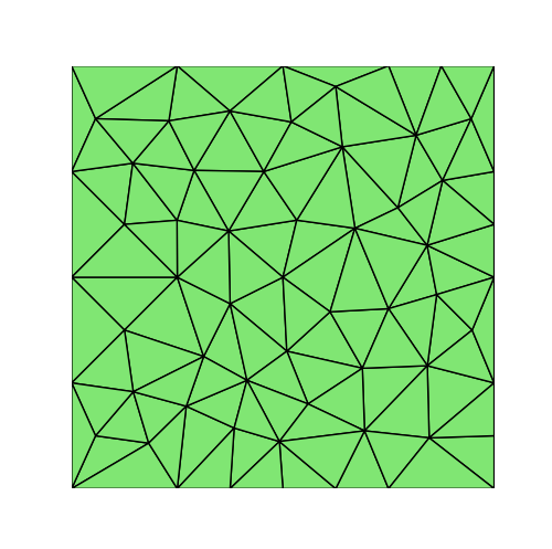
In this section, we first introduce a fixed-point algorithm (Oseen iteration) for the handing of nonlinear problems. Next, by the Example 5.1, we verify the convergence rates of the proposed nonconforming VEM for the cases $k=1,2$ , and compare the nonconforming VEM, the conforming VEM and the FEM for the case $k=1$ . The above conforming VEM only changes the approximation space of the velocity compared with the nonconforming VEM, the velocity is approximate by the low-order Stokes-type virtual element [30]. For the FEM, the stable finite element pair $(P_{1b},P_{1},P_{1})$ is used for discretization. For both the VEM and FEM, we adopt Oseen iteration to deal with nonlinear system. The Oseen iteration scheme of the VEM is as follows:

\displaystyle\begin{cases}A_{h}(\boldsymbol{\boldsymbol{u}}_{h}^{n},\boldsymbol{b}_{h}^{n};\boldsymbol{v}_{h},\boldsymbol{c}_{h})+B_{h}(\boldsymbol{u}_{h}^{n-1},\boldsymbol{b}_{h}^{n-1};\boldsymbol{u}_{h}^{n},\boldsymbol{b}_{h}^{n};\boldsymbol{v}_{h},\boldsymbol{c}_{h})-d_{h}(\boldsymbol{v}_{h},\boldsymbol{c}_{h};p_{h}^{n})=\left<F_{h};\boldsymbol{v}_{h},\boldsymbol{c}_{h}\right>,\\ d_{h}(\boldsymbol{u}_{h}^{n},\boldsymbol{b}_{h}^{n};q_{h})=0,\end{cases}

with the iterative initial value $\boldsymbol{u}_{h}^{0}=\mathbf{0},\boldsymbol{b}_{h}^{0}=\mathbf{0}$ , the iterative tolerance is 1e-7. The Oseen iteration of the FEM can be found in [18]. Then, in Example 5.2, we investigate a benchmark problem. All experiments are implemented with FEALPy package [33].

In order to compute VEM errors, we consider the following computable error quantities:

	$\displaystyle\\|e_{\boldsymbol{u}}\\|_{0}$	$\displaystyle=\sqrt{\sum_{E\in\mathcal{T}_{h}}\\|\boldsymbol{u}-\Pi_{k}^{0,E}\boldsymbol{u}_{h}\\|_{0,E}^{2}},\quad\|e_{\boldsymbol{u}}\|_{1}=\sqrt{\sum_{E\in\mathcal{T}_{h}}\|\boldsymbol{u}-\Pi_{k}^{\nabla,E}\boldsymbol{u}_{h}\|_{1,E}^{2}},\quad\\|e_{p}\\|_{0}=\\|p-p_{h}\\|_{0},$
	$\displaystyle\\|e_{\boldsymbol{b}}\\|_{0}$	$\displaystyle=\sqrt{\sum_{E\in\mathcal{T}_{h}}\\|\boldsymbol{b}-\Pi_{k}^{0,E}\boldsymbol{b}_{h}\\|_{0,E}^{2}},\quad\\|e_{\boldsymbol{b}}\\|_{1}=\sqrt{\sum_{E\in\mathcal{T}_{h}}\big{(}\\|\boldsymbol{b}-\Pi_{k}^{0,E}\boldsymbol{b}_{h}\\|_{0,E}^{2}+\|\boldsymbol{b}-\Pi_{k}^{\nabla,E}\boldsymbol{b}_{h}\|_{1,E}^{2}\big{)}}.$

For the choice of the stabilization terms $\mathrm{S}_{0}^{E},\mathrm{S}_{1}^{E}$ , we follow [34, 2]

	$\displaystyle\mathrm{S}_{0}^{E}(\boldsymbol{u}_{h},\boldsymbol{v}_{h})=\sum_{i=1}^{\mathrm{dim}(\boldsymbol{V}(E))}\mathrm{dof}_{i}^{\boldsymbol{V}(E)}(\boldsymbol{u}_{h})\mathrm{dof}_{i}^{\boldsymbol{V}(E)}(\boldsymbol{v}_{h}),$
	$\displaystyle\mathrm{S}_{1}^{E}(\boldsymbol{b}_{h},\boldsymbol{c}_{h})=\sum_{i=1}^{\mathrm{dim}(\boldsymbol{M}(E))}\mathrm{dof}_{i}^{\boldsymbol{M}(E)}(\boldsymbol{b}_{h})\mathrm{dof}_{i}^{\boldsymbol{M}(E)}(\boldsymbol{c}_{h}),$

where $\mathrm{dof}_{i}^{\boldsymbol{W}}(\boldsymbol{v})$ is the $i$ th degree of freedom of smooth enough function $\boldsymbol{v}$ to the space $\boldsymbol{W}$ , here $\boldsymbol{W}$ is $\boldsymbol{V}(E)$ or $\boldsymbol{M}(E)$ . Of course, the choice is not unique, there are also some other options [29, 11, 13].

Refer to caption — Figure 1: Sample meshes: $\mathcal{T}_{h}^{1}$ (left), $\mathcal{T}_{h}^{2}$ (middle) and $\mathcal{T}_{h}^{3}$ (right).

Example 5.1

We consider solving MHD with $R_{\nu}=R_{m}=S_{c}=1$ on domain $\Omega=[0,1]^{2}$ . The source terms $\boldsymbol{f}$ and $\boldsymbol{g}$ satisfy the exact solutions

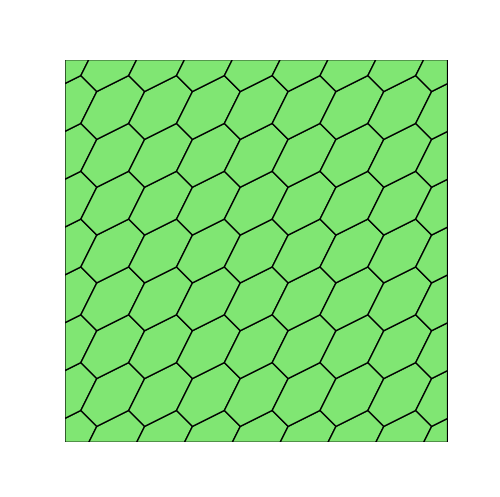
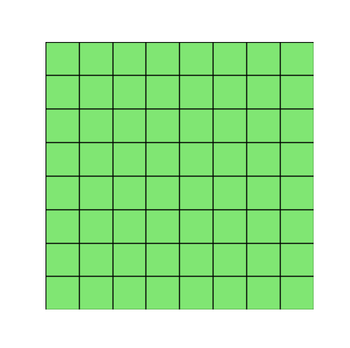
\displaystyle\boldsymbol{u}=\begin{pmatrix}\sin(\pi x_{1})^{2}\sin(\pi x_{2})\cos(\pi x_{2})\\ -\sin(\pi x_{1})\sin(\pi x_{2})^{2}\cos(\pi x_{1})\end{pmatrix},\;\boldsymbol{b}=\begin{pmatrix}\sin(\pi x_{1})\cos(\pi x_{2})\\ -\sin(\pi x_{2})\cos(\pi x_{1})\end{pmatrix},\;p=\cos(\pi x_{1})\cos(\pi x_{2}).

In Table 1, we list the errors and the optimal convergence rates of the velocity on meshes $\mathcal{T}_{h}^{1}$ and $\mathcal{T}_{h}^{2}$ (see Figure 1) for the cases $k=1,2$ , as well as $L^{2}$ -norm of $\mathrm{div}_{h}\boldsymbol{u}_{h}$ . We observe that the discrete velocity is divergence-free up to machine precision. Table 2 displays the errors and the optimal convergence rates of the magnetic and pressure on meshes $\mathcal{T}_{h}^{1}$ and $\mathcal{T}_{h}^{2}$ for the cases $k=1,2$ . Tables 1 and 2 illustrate validity of the theoretical analysis.

Table 1: Convergence rates of velocity on meshes

\mathcal{T}_{h}^{1}

and

\mathcal{T}_{h}^{2}

meshes	$k$	$h$	$\\|e_{\boldsymbol{u}}\\|_{0}$	Rate	$\|e_{\boldsymbol{u}}\|_{1}$	Rate	$\\|\mathrm{div}_{h}\boldsymbol{u}_{h}\\|_{0}$
$\mathcal{T}_{h}^{1}$	1	0.3727	7.9642e-02	-	1.4316e+00	-	1.8392e-15
		0.1863	2.7525e-02	1.53	7.0057e-01	1.03	3.6925e-15
		0.0932	7.8488e-03	1.81	3.3440e-01	1.07	2.7869e-15
		0.0466	2.0667e-03	1.93	1.6374e-01	1.03	1.1629e-14
		0.0233	5.2739e-04	1.97	8.1386e-02	1.01	4.7360e-14
$\mathcal{T}_{h}^{1}$	2	0.3727	2.8702e-02	-	1.4227e+00	-	6.2575e-15
		0.1863	3.7358e-03	2.94	5.5399e-01	1.36	1.1871e-14
		0.0932	4.2119e-04	3.15	1.5298e-01	1.86	2.5457e-14
		0.0466	4.4875e-05	3.23	3.9484e-02	1.95	4.4265e-14
		0.0233	4.9710e-06	3.17	9.9924e-03	1.98	1.2225e-13
$\mathcal{T}_{h}^{2}$	1	0.3536	1.5356e-01	-	1.6980e+00	-	1.0977e-15
		0.1768	4.4590e-02	1.78	7.6794e-01	1.14	3.0290e-15
		0.0884	1.1317e-02	1.98	3.3497e-01	1.2	3.9649e-15
		0.0442	2.8199e-03	2.0	1.5790e-01	1.09	8.4733e-15
		0.0221	7.0356e-04	2.0	7.7581e-02	1.03	3.3386e-14
$\mathcal{T}_{h}^{2}$	2	0.3536	5.6481e-02	-	1.5316e+00	-	8.3672e-15
		0.1768	9.0257e-03	2.65	8.8572e-01	0.79	8.7864e-15
		0.0884	9.1090e-04	3.31	3.0408e-01	1.54	1.5897e-14
		0.0442	7.7982e-05	3.55	8.2445e-02	1.88	4.1011e-14
		0.0221	6.5169e-06	3.58	2.1539e-02	1.94	1.1272e-13

Table 2: Convergence rates of magnetic field and pressure on meshes

\mathcal{T}_{h}^{1}

and

\mathcal{T}_{h}^{2}

meshes	$k$	$h$	$\\|e_{\boldsymbol{b}}\\|_{0}$	Rate	$\\|e_{\boldsymbol{b}}\\|_{1}$	Rate	$\\|e_{p}\\|_{0}$	Rate
$\mathcal{T}_{h}^{1}$	1	0.3727	4.7679e-02	-	9.1759e-01	-	3.5180e-01	-
		0.1863	1.3848e-02	1.78	4.9783e-01	0.88	1.7097e-01	1.04
		0.0932	3.7189e-03	1.9	2.5769e-01	0.95	6.4053e-02	1.42
		0.0466	9.5814e-04	1.96	1.3086e-01	0.98	2.5234e-02	1.34
		0.0233	2.4266e-04	1.98	6.5904e-02	0.99	1.1266e-02	1.16
$\mathcal{T}_{h}^{1}$	2	0.3727	7.6370e-03	-	1.7843e-01	-	1.8498e-01	-
		0.1863	1.0430e-03	2.87	4.8383e-02	1.88	4.9715e-02	1.9
		0.0932	1.3037e-04	3.0	1.2346e-02	1.97	9.4398e-03	2.4
		0.0466	1.6216e-05	3.01	3.1185e-03	1.99	1.5328e-03	2.62
		0.0233	2.0260e-06	3.0	7.8440e-04	1.99	2.5201e-04	2.6
$\mathcal{T}_{h}^{2}$	1	0.3536	7.8227e-02	-	9.9789e-01	-	3.1471e-01	-
		0.1768	1.9856e-02	1.98	5.0244e-01	0.99	1.5002e-01	1.07
		0.0884	4.9809e-03	2.0	2.5167e-01	1.0	5.6183e-02	1.42
		0.0442	1.2462e-03	2.0	1.2589e-01	1.0	2.2761e-02	1.3
		0.0221	3.1162e-04	2.0	6.2955e-02	1.0	1.0399e-02	1.13
$\mathcal{T}_{h}^{2}$	2	0.3536	6.3629e-03	-	1.9293e-01	-	7.4471e-01	-
		0.1768	8.0376e-04	2.98	4.8794e-02	1.98	2.0652e-01	1.85
		0.0884	9.6233e-05	3.06	1.2098e-02	2.01	3.4511e-02	2.58
		0.0442	1.1679e-05	3.04	3.0013e-03	2.01	5.1169e-03	2.75
		0.0221	1.4478e-06	3.01	7.4778e-04	2.0	9.0330e-04	2.5

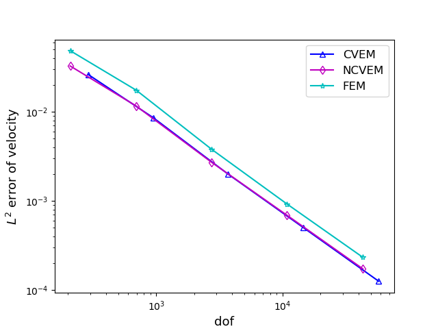
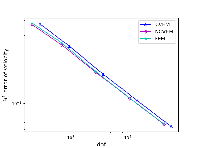
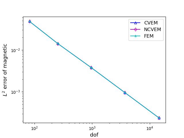
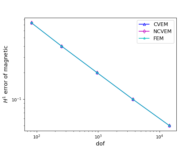
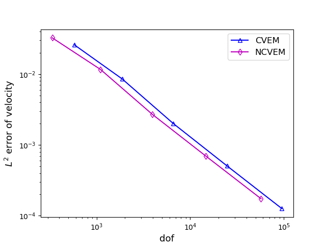
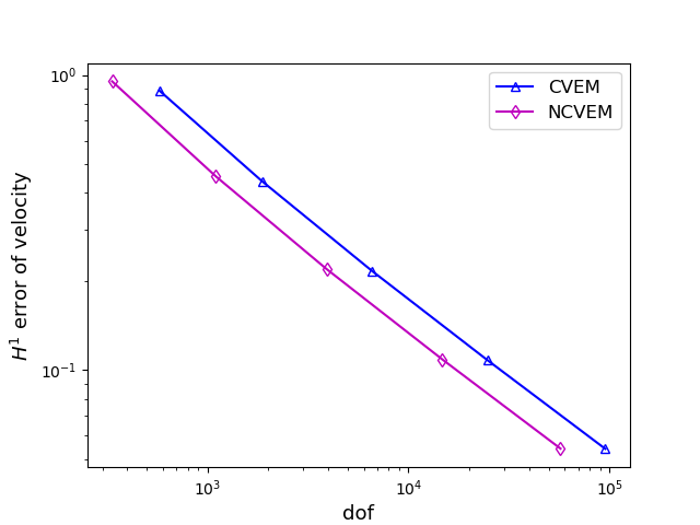
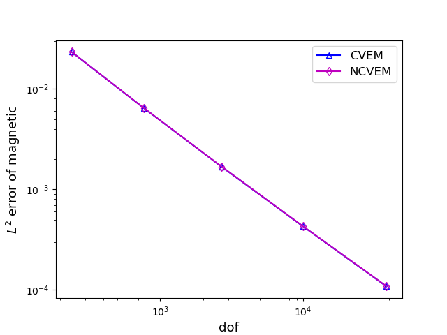
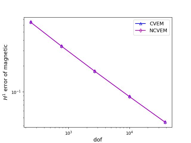
For comparison, we also solve the MHD problem by the conforming VEM and the FEM. In Figure 2, we compare with three methods on meshes $\mathcal{T}_{h}^{3}$ for the case $k=1$ , by displaying the error curves of the velocity and magnetic field with respect to the number of degrees of freedom. Figure 3 shows the compared results of the conforming VEM and the nonconforming VEM on meshes $\mathcal{T}_{h}^{1}$ for the case $k=1$ . From Figures 2 and 3, we observe that our proposed nonconforming VEM can provide better approximations for the velocity than the conforming VEM and the FEM in the numerical test for the case $k=1$ .

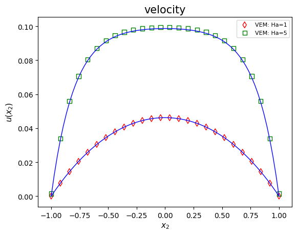
Example 5.2

We consider Hartmann flow in the channel $\Omega=[0,6]\times[-1,1]$ . The transverse magnetic field $\boldsymbol{b}_{d}=(0,1)$ is applied. The solutions of MHD are

\displaystyle\boldsymbol{u}(x_{1},x_{2})=(u(x_{2}),0),\quad\boldsymbol{b}(x_{1},x_{2})=(b(x_{2}),1),\quad p(x_{1},x_{2})=-Gx_{1}-S_{c}b^{2}(x_{2})/2,

where

\displaystyle u(x_{2})=\frac{GR_{\nu}}{\mathrm{Ha}\cdot\tanh(\mathrm{Ha})}\left(1-\frac{\cosh(x_{2}\mathrm{Ha})}{\cosh(\mathrm{Ha})}\right),\quad b(x_{2})=\frac{G}{S_{c}}\left(\frac{\sinh(x_{2}\mathrm{Ha})}{\sinh(\mathrm{Ha})}-x_{2}\right).

$\mathrm{Ha}=\sqrt{R_{\nu}R_{m}S_{c}}$ is the Hartmann number, $\boldsymbol{f}=\boldsymbol{g}=\boldsymbol{0}$ , and boundary conditions are given by

	$\displaystyle\boldsymbol{u}=\boldsymbol{0}\quad\mathrm{on}\;x_{2}=\pm 1,$
	$\displaystyle(p\mathrm{I}-R_{\nu}^{-1}\nabla\boldsymbol{u})\boldsymbol{n}=p\boldsymbol{n}\quad\mbox{on}\;x_{1}=0\;\mbox{and}\;x_{1}=6,$
	$\displaystyle\boldsymbol{n}\times\boldsymbol{b}=\boldsymbol{n}\times\boldsymbol{b}_{d}\quad\mbox{on}\;\partial\Omega.$

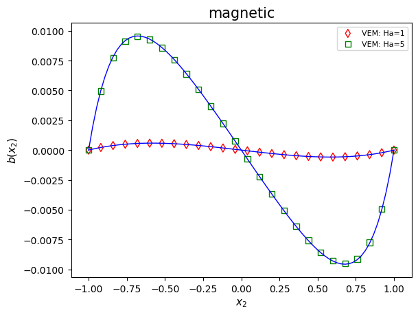
Without loss of generality, we set $G=0.1$ . The numerical experiment is carried out on meshes $\mathcal{T}_{h}^{2}$ with $h=0.358$ . Figure 4 presents the first components of numerical solutions ( $L^{2}$ -projection) and analytical solutions with $\mathrm{Ha}=1$ ( $R_{\nu}=1,R_{m}=0.1,S_{c}=10$ ) and $\mathrm{Ha}=5$ ( $R_{\nu}=5,R_{m}=1,S_{c}=5$ ). The experiment indicates that the numerical solutions almost agree with the analytical solutions.

Acknowledgements

The research was supported by the National Natural Science Foundation of China (Nos: 12071404, 11971410, 12026254), Young Elite Scientist Sponsorship Program by CAST (No: 2020QNRC001), the Science and Technology Innovation Program of Hunan Province (No: 2024RC3158), Key Project of Scientific Research Project of Hunan Provincial Department of Education (No: 22A0136), Postgraduate Scientific Research Innovation Project of Hunan Province (No: CX20230614).

References

[1] D. Adak, D. Mora, S. Natarajan, and A. Silgado. A virtual element discretization for the time dependent Navier–Stokes equations in stream-function formulation. ESAIM: Mathematical Modelling and Numerical Analysis, 55(5):2535–2566, 2021.
[2] B. Ahmad, A. Alsaedi, F. Brezzi, L. D. Marini, and A. Russo. Equivalent projectors for virtual element methods. Computers $\&$ Mathematics with Applications, 66(3):376–391, 2013.
[3] S. N. Alvarez, V. Bokil, V. Gyrya, and G. Manzini. The virtual element method for resistive magnetohydrodynamics. Computer Methods in Applied Mechanics and Engineering, 381:113815, 2021.
[4] P. F. Antonietti, L. Beirão da Veiga, D. Mora, and M. Verani. A stream virtual element formulation of the Stokes problem on polygonal meshes. SIAM Journal on Numerical Analysis, 52(1):386–404, 2014.
[5] L. Beirão da Veiga, F. Brezzi, A. Cangiani, G. Manzini, L. D. Marini, and A. Russo. Basic principles of virtual element methods. Mathematical Models and Methods in Applied Sciences, 23(01):199–214, 2013.
[6] L. Beirão da Veiga, F. Brezzi, L. D. Marini, and A. Russo. The hitchhiker’s guide to the virtual element method. Mathematical Models and Methods in Applied Sciences, 24(08):1541–1573, 2014.
[7] L. Beirão da Veiga, F. Dassi, G. Manzini, and L. Mascotto. The virtual element method for the 3D resistive magnetohydrodynamic model. Mathematical Models and Methods in Applied Sciences, 33(03):643–686, 2023.
[8] L. Beirão da Veiga, C. Lovadina, and G. Vacca. Divergence free virtual elements for the Stokes problem on polygonal meshes. ESAIM: Mathematical Modelling and Numerical Analysis, 51(2):509–535, 2017.
[9] L. Beirão da Veiga, C. Lovadina, and G. Vacca. Virtual elements for the Navier–Stokes problem on polygonal meshes. SIAM Journal on Numerical Analysis, 56(3):1210–1242, 2018.
[10] S. C. Brenner. The mathematical theory of finite element methods. Springer, 2008.
[11] S. C. Brenner and L.-Y. Sung. Virtual element methods on meshes with small edges or faces. Mathematical Models and Methods in Applied Sciences, 28(07):1291–1336, 2018.
[12] A. Cangiani, V. Gyrya, and G. Manzini. The nonconforming virtual element method for the Stokes equations. SIAM Journal on Numerical Analysis, 54(6):3411–3435, 2016.
[13] L. Chen and J. Huang. Some error analysis on virtual element methods. Calcolo, 55:1–23, 2018.
[14] C. Cuvelier, A. Segal, and A. A. Van Steenhoven. Finite element methods and Navier-Stokes equations, volume 22. Springer Science & Business Media, 1986.
[15] P. A. Davidson. Introduction to magnetohydrodynamics, volume 55. Cambridge university press, 2017.
[16] B. A. De Dios, K. Lipnikov, and G. Manzini. The nonconforming virtual element method. ESAIM: Mathematical Modelling and Numerical Analysis, 50(3):879–904, 2016.
[17] X. Dong and Y. He. Two-level newton iterative method for the 2D/3D stationary incompressible magnetohydrodynamics. Journal of Scientific Computing, 63(2):426–451, 2015.
[18] X. Dong, Y. He, and Y. Zhang. Convergence analysis of three finite element iterative methods for the 2D/3D stationary incompressible magnetohydrodynamics. Computer Methods in Applied Mechanics and Engineering, 276:287–311, 2014.
[19] J.-F. Gerbeau, C. Le Bris, and T. Lelièvre. Mathematical methods for the magnetohydrodynamics of liquid metals. Clarendon Press, 2006.
[20] C. Greif, D. Li, D. Schötzau, and X. Wei. A mixed finite element method with exactly divergence-free velocities for incompressible magnetohydrodynamics. Computer Methods in Applied Mechanics and Engineering, 199(45-48):2840–2855, 2010.
[21] M. D. Gunzburger, A. J. Meir, and J. S. Peterson. On the existence, uniqueness, and finite element approximation of solutions of the equations of stationary, incompressible magnetohydrodynamics. Mathematics of Computation, 56(194):523–563, 1991.
[22] R. Hiptmair, L. Li, S. Mao, and W. Zheng. A fully divergence-free finite element method for magnetohydrodynamic equations. Mathematical Models and Methods in Applied Sciences, 28(04):659–695, 2018.
[23] K. Hu, Y. Ma, and J. Xu. Stable finite element methods preserving $\nabla\cdot$ B= 0 exactly for mhd models. Numerische Mathematik, 135(2):371–396, 2017.
[24] K. Hu and J. Xu. Structure-preserving finite element methods for stationary MHD models. Mathematics of Computation, 88(316):553–581, 2019.
[25] H. Huang, Y. Huang, and X. Dong. Three interior penalty DG methods for stationary incompressible magnetohydrodynamics. Journal of Computational and Applied Mathematics, 425:115030, 2023.
[26] O. A. Karakashian and W. N. Jureidini. A nonconforming finite element method for the stationary Navier–Stokes equations. SIAM Journal on Numerical Analysis, 35(1):93–120, 1998.
[27] X. Liu and Z. Chen. The nonconforming virtual element method for the Navier-Stokes equations. Advances in Computational Mathematics, 45:51–74, 2019.
[28] X. Liu, J. Li, and Z. Chen. A nonconforming virtual element method for the Stokes problem on general meshes. Computer Methods in Applied Mechanics and Engineering, 320:694–711, 2017.
[29] L. Mascotto. Ill-conditioning in the virtual element method: Stabilizations and bases. Numerical Methods for Partial Differential Equations, 34(4):1258–1281, 2018.
[30] S. Naranjo-Alvarez, L. Beirão da Veiga, V. A. Bokil, F. Dassi, V. Gyrya, and G. Manzini. The virtual element method for a 2D incompressible MHD system. Mathematics and Computers in Simulation, 211:301–328, 2023.
[31] Q. Tang and Y. Huang. Local and parallel finite element algorithm based on Oseen-type iteration for the stationary incompressible MHD flow. Journal of Scientific Computing, 70:149–174, 2017.
[32] H. Wei, X. Huang, and A. Li. Piecewise divergence-free nonconforming virtual elements for Stokes problem in any dimensions. SIAM Journal on Numerical Analysis, 59(3):1835–1856, 2021.
[33] H. Wei and Y. Huang. Fealpy: Finite Element Analysis Library in Python. https://github.com/weihuayi/ fealpy, Xiangtan University, 2017-2023.
[34] B. Zhang, J. Zhao, and M. Li. The divergence-free nonconforming virtual element method for the Navier–Stokes problem. Numerical Methods for Partial Differential Equations, 39(3):1977–1995, 2023.
[35] J. Zhao, B. Zhang, S. Mao, and S. Chen. The divergence-free nonconforming virtual element for the Stokes problem. SIAM Journal on Numerical Analysis, 57(6):2730–2759, 2019.

$\displaystyle\|A(\boldsymbol{u},\boldsymbol{b};\boldsymbol{v},\boldsymbol{c})\|$	$\displaystyle\leq\max\left\{R_{\nu}^{-1},4R_{m}^{-1}S_{c}\right\}\\|(\boldsymbol{u},\boldsymbol{b})\\|_{1}\,\\|(\boldsymbol{v},\boldsymbol{c})\\|_{1},$	(2.5)
$\displaystyle A(\boldsymbol{u},\boldsymbol{b};\boldsymbol{u},\boldsymbol{b})$	$\displaystyle\geq\min\{R_{\nu}^{-1},\lambda_{1}R_{m}^{-1}S_{c}\}\\|(\boldsymbol{u},\boldsymbol{b})\\|_{1}^{2},$	(2.6)
$\displaystyle\|B(\boldsymbol{u},\boldsymbol{b};\boldsymbol{w},\boldsymbol{\psi};\boldsymbol{v},\boldsymbol{c})\|$	$\displaystyle\leq\sqrt[]{2}\lambda_{0}^{2}\max\{1,\sqrt[]{2}S_{c}\}\\|(\boldsymbol{u},\boldsymbol{b})\\|_{1}\,\\|(\boldsymbol{w},\boldsymbol{\psi})\\|_{1}\,\\|(\boldsymbol{v},\boldsymbol{c})\\|_{1}.$	(2.7)

	$\displaystyle\\|(\mathrm{I}-\Pi_{k-1}^{0,E})\mathrm{curl}\,\boldsymbol{c}_{h}\\|_{0,E}$	$\displaystyle\leq\\|\mathrm{curl}\,(\mathrm{I}-\Pi_{k}^{\nabla,E})\boldsymbol{c}_{h}\\|_{0,E}\leq\sqrt{2}\\|\nabla(\mathrm{I}-\Pi_{k}^{\nabla,E})\boldsymbol{c}_{h}\\|_{0,E},$
	$\displaystyle\\|(\mathrm{I}-\Pi_{k-1}^{0,E})\mathrm{div}\,\boldsymbol{c}_{h}\\|_{0,E}$	$\displaystyle\leq\\|\mathrm{div}\,(\mathrm{I}-\Pi_{k}^{\nabla,E})\boldsymbol{c}_{h}\\|_{0,E}\leq\sqrt{2}\\|\nabla(\mathrm{I}-\Pi_{k}^{\nabla,E})\boldsymbol{c}_{h}\\|_{0,E},$

	$\displaystyle a_{1h}^{E}(\boldsymbol{c}_{h},\boldsymbol{c}_{h})$	$\displaystyle\leq R_{m}^{-1}S_{c}\left(\\|\Pi_{k-1}^{0,E}\mathrm{curl}\,\boldsymbol{c}_{h}\\|_{0,E}^{2}+\\|\Pi_{k-1}^{0,E}\mathrm{div}\,\boldsymbol{c}_{h}\\|_{0,E}^{2}+\alpha_{1}^{\ast}\\|\nabla(\mathrm{I}-\Pi_{k}^{\nabla,E})\boldsymbol{c}_{h}\\|_{0,E}^{2}\right)$
		$\displaystyle\leq R_{m}^{-1}S_{c}(4+\alpha_{1}^{\ast})\\|\boldsymbol{c}_{h}\\|_{1,E}^{2}=R_{m}^{-1}S_{c}\sigma_{1}^{\ast}\\|\boldsymbol{c}_{h}\\|_{1,E}^{2}$
	$\displaystyle a_{1h}^{E}(\boldsymbol{c}_{h},\boldsymbol{c}_{h})$	$\displaystyle\geq R_{m}^{-1}S_{c}\left(\\|\Pi_{k-1}^{0,E}\mathrm{curl}\,\boldsymbol{c}_{h}\\|_{0,E}^{2}+\\|\Pi_{k-1}^{0,E}\mathrm{div}\,\boldsymbol{c}_{h}\\|_{0,E}^{2}+\alpha_{1\ast}\\|\nabla(\mathrm{I}-\Pi_{k}^{\nabla,E})\boldsymbol{c}_{h}\\|_{0,E}^{2}\right)$
		$\displaystyle\geq R_{m}^{-1}S_{c}\Big{(}\\|\Pi_{k-1}^{0,E}\mathrm{curl}\,\boldsymbol{c}_{h}\\|_{0,E}^{2}+\\|\Pi_{k-1}^{0,E}\mathrm{div}\,\boldsymbol{c}_{h}\\|_{0,E}^{2}+\frac{\alpha_{1\ast}}{4}\Big{(}\\|(\mathrm{I}-\Pi_{k-1}^{0,E})\mathrm{curl}\,\boldsymbol{c}_{h}\\|_{0,E}^{2}$
		$\displaystyle\quad+\\|(\mathrm{I}-\Pi_{k-1}^{0,E})\mathrm{div}\,\boldsymbol{c}_{h}\\|_{0,E}^{2}\Big{)}\Big{)}$
		$\displaystyle\geq R_{m}^{-1}S_{c}\min\{1,\frac{\alpha_{1\ast}}{4}\}\big{(}\\|\mathrm{curl}\,\boldsymbol{c}_{h}\\|_{0,E}^{2}+\\|\mathrm{div}\,\boldsymbol{c}_{h}\\|_{0,E}^{2}\big{)}=\sigma_{1\ast}a_{1}^{E}(\boldsymbol{c}_{h},\boldsymbol{c}_{h}).$

	$\displaystyle\|A_{h}(\boldsymbol{u}_{h},\boldsymbol{b}_{h};\boldsymbol{v}_{h},\boldsymbol{c}_{h})\|$	$\displaystyle=\|a_{0h}(\boldsymbol{u}_{h},\boldsymbol{v}_{h})+a_{1h}(\boldsymbol{b}_{h},\boldsymbol{c}_{h})\|$
		$\displaystyle\leq\sum_{E\in\mathcal{T}_{h}}\left(\sigma_{0}^{\ast}R_{\nu}^{-1}\|\boldsymbol{u}_{h}\|_{1,E}\|\boldsymbol{v}_{h}\|_{1,E}+\sigma_{1}^{\ast}R_{m}^{-1}S_{c}\\|\boldsymbol{b}_{h}\\|_{1,E}\\|\boldsymbol{c}_{h}\\|_{1,E}\right)$
		$\displaystyle\leq\sigma^{\ast}\max\{R_{\nu}^{-1},R_{m}^{-1}S_{c}\}\\|(\boldsymbol{u}_{h},\boldsymbol{b}_{h})\\|_{1,h}\,\\|(\boldsymbol{v}_{h},\boldsymbol{c}_{h})\\|_{1,h}.$

	$\displaystyle\sup_{(\boldsymbol{v}_{I},\boldsymbol{c}_{h})\in\boldsymbol{V}\times\boldsymbol{M}}\frac{\|d_{h}(\boldsymbol{v}_{I},\boldsymbol{c}_{h};q_{h})\|}{\\|(\boldsymbol{v}_{I},\boldsymbol{c}_{h})\\|_{1,h}}$	$\displaystyle\geq\sup_{(\boldsymbol{v}_{I},\boldsymbol{c}_{h})\in\boldsymbol{V}\times\boldsymbol{0}}\frac{\|d_{h}(\boldsymbol{v}_{I},\boldsymbol{c}_{h};q_{h})\|}{\\|(\boldsymbol{v}_{I},\boldsymbol{c}_{h})\\|_{1,h}}$
		$\displaystyle=\sup_{\boldsymbol{v}_{I}\in\boldsymbol{V}}\frac{\|(\mathrm{div}\,\boldsymbol{v},q_{h})\|}{\|\boldsymbol{v}_{I}\|_{1,h}}$
		$\displaystyle\geq\frac{1}{\eta}\sup_{\boldsymbol{v}\in\boldsymbol{H}_{0}^{1}(\Omega)}\frac{\|(\mathrm{div}\,\boldsymbol{v},q_{h})\|}{\|\boldsymbol{v}\|_{1}}\geq\frac{\gamma_{0}}{\eta}\\|q_{h}\\|_{0}=\gamma_{1}\\|q_{h}\\|_{0}.$

Conservative nonconforming virtual element method for stationary incompressible magnetohydrodynamics ††thanks: .

Abstract

1 Introduction

2 Preliminaries

Theorem 2.1

3 Virtual element method

3.1 Meshes and projections

3.2 The nonconforming element space and piecewise polynomials space

Lemma 3.1

3.3 The nodal space

Lemma 3.2

Lemma 3.3

3.4 The discrete formulation

Lemma 3.4

Lemma 3.5

Lemma 3.6

Theorem 3.1

4 Error analysis

Lemma 4.1

Lemma 4.2

Theorem 4.1

Theorem 4.2

5 Numerical examples

Example 5.1

Example 5.2

Acknowledgements

References

Conservative nonconforming virtual element method for stationary incompressible magnetohydrodynamics ^†^†thanks: .