Conformal Depression Prediction
Abstract
While existing depression prediction methods based on deep learning show promise, their practical application is hindered by the lack of trustworthiness, as these deep models are often deployed as black box models, leaving us uncertain on the confidence of their predictions. For high-risk clinical applications like depression prediction, uncertainty quantification is essential in decision-making. In this paper, we introduce conformal depression prediction (CDP), a depression prediction method with uncertainty quantification based on conformal prediction (CP), giving valid confidence intervals with theoretical coverage guarantees for the model predictions. CDP is a plug-and-play module that requires neither model retraining nor an assumption about the depression data distribution. As CDP provides only an average coverage guarantee across all inputs rather than per-input performance guarantee, we further propose CDP-ACC, an improved conformal prediction with approximate conditional coverage. CDP-ACC firstly estimates the prediction distribution through neighborhood relaxation, and then introduces a conformal score function by constructing nested sequences, so as to provide a tighter prediction interval adaptive to specific input. We empirically demonstrate the application of CDP in uncertainty-aware facial depression prediction, as well as the effectiveness and superiority of CDP-ACC on the AVEC 2013 and AVEC 2014 datasets. Our code is publicly available at https://github.com/PushineLee/CDP.
Index Terms:
facial depression prediction, uncertainty quantification, conformal prediction, approximate conditional coverage.I Introduction
Depression is a prevalent mental disorder presented as persistent feelings of sadness, debilitation, and loss of interest in activities [1, 2, 3]. It increases the risk of suicide and accounts for a substantial psychological burden [4, 5]. The existing primary diagnostic methods used involve mental health reports, such as the Beck Depression Inventory (BDI-II) [6] (target variable focused on in this paper), the Hamilton Depression Rating Scale (HRSD) [7], and the Patient Health Questionnaire (PHQ-8) [8]. The diagnostic process depends on interviews and demands considerable time and effort from both psychiatrists and patients. Also, it heavily relies on the clinicians’ subjective experience, as well as the patients’ cognitive abilities and psychological states.
Over the past decade, continuous efforts have been made to explore effective biomarkers and methods for automated depression prediction. For depression biomarkers, initial attention was focused on hand-crafted features such as Local Binary Patterns (LBP) [9], Local Gabor Binary Patterns from Three Orthogonal Planes (LGBP-TOP) [10], and Local Binary Pattern from Three Orthogonal Planes (LBP-TOP) [11, 12] extracted from facial videos. Handcrafted features extracted from other behavioral signals have also been employed in this task, including speech, facial action units, facial landmarks, head poses, and gazes [13, 14]. The development of these hand-crafted features heavily relies on specific knowledge related to the depression prediction tasks. Acquiring such knowledge is time-consuming, subject to researchers’ subjective cognition and task specificity, and lacks good generalization. Moreover, these features struggle to identify certain implicit and difficult-to-distinguish patterns of depression [15]. Fortunately, with the advent of deep learning [16], a new pathway has been opened for depression prediction tasks. In this pipeline end-to-end deep neural networks can be trained using depression data including facial video [17, 18, 19, 20], speech [21, 22, 13] and other data sources. These deep models are expected to discover subtle, indistinguishable depression-related features and implicitly discriminate among them for improved prediction.

While the rapid development of deep learning and computer vision has led to exciting progress in depression prediction, the reliability and trustworthiness of deep learning models-considered black boxes [23, 24, 25]-have not been well addressed. These models may exhibit overconfidence in predicting failures, potentially leading to catastrophic risks. For automated depression prediction, the accuracy performance should not be the only criterion determining the usefulness of a predictive model. The lack of statistically rigorous uncertainty quantification is a key factor undermining the reliability of depression prediction. Consider the application context of depression prediction. We are more willing to accept reliable predictions that provide insight into potential risks. Beyond the depression severity prediction, we need additional outcomes to represent their uncertainty. As shown in Fig. 1, our aim is to provide statistically rigorous confidence intervals in depression prediction. These intervals should cover the actual depression scores with any user-defined level of confidence.
In this work, we propose conformal depression prediction (CDP) to quantify the uncertainty of depression severity estimation based on conformal prediction (CP [26, 27]). CDP can provide confidence intervals to satisfy marginal coverage for the actual depression scores. We show that, CDP as a plug-and-play module, can validly quantify uncertainty for most depression prediction models, without retraining the model. Furthermore, inspired by the adaptive prediction sets (APS) [28] in uncertainty-aware classification tasks, which construct a prediction set per-input adaptive to its prediction distribution, we propose conformal depression prediction with approximate conditional coverage (CDP-ACC) to overcome the shortcomings of conformal prediction with marginal coverage, providing adaptive confidence intervals for depression prediction.
The main contributions are summarized as follows:
1. We propose an uncertainty quantification framework CDP for facial depression prediction. CDP provides statistically rigorous confidence intervals that satisfy marginal coverage for most existing facial depression prediction models.
2. We develop CDP-ACC, an improved CDP algorithm that satisfies approximate conditional coverage, yielding tighter confidence intervals while maintaining good coverage.
3. We conduct extensive experiments to demonstrate the effectiveness of our proposed method in uncertainty quantification of facial depression prediction.
II RELATED WORK
II-A Depression Prediction
Over the past decade, depression prediction based on deep learning has attracted significant interest and attention in the field, leading to many meaningful research advancements. Studies using labeled depression data from various modalities, including speech, text, video, and EEG signals, as well as the integration of these modalities, have taken a leading role.
For single-modality depression prediction, He et al. employed a Deep Convolutional Neural Network (DCNN) to extract depression-related features from speech data [21]. These learned features were subsequently integrated with additional hand-crafted features to predict depression scores. Zhao et al. introduced a hybrid network that integrates Self-Attention Networks (SAN) and DCNN to handle both low-level acoustic features and 3D Log-Mel spectrogram data [22]. Following this, feature fusion techniques along with support vector regression are employed for depression prediction. Melo et al. concentrated on efficiently extracting spatiotemporal features from facial videos associated with depression [17, 18]. They introduced a deep Multiscale Spatiotemporal Network (MSN) and a deep Maximization-Differentiation Network (MDN) to predict depression levels. Sharma et al. proposed CNN-LSTM hybrid networks to extract depression features from EEG signals [29]. Seal et al. developed the DeprNet, a DCNN designed for classification of EEG data from depressed and normal subjects [30].
For multimodal depression prediction, Niu et al. introduced a novel Spatio-Temporal Attention (STA) network and a Multimodal Attention Feature Fusion (MAFF) strategy to acquire a multimodal representation of depression cues from facial and speech spectrum [31]. Uddin et al. introduced a novel deep multi-modal framework that effectively integrates facial and verbal cues for automated depression prediction [32]. They extracted features separately from video and speech and employed a Multi-modal Factorized Bilinear pooling (MFB) strategy to efficiently fuse these multi-modal features. Niu et al. proposed a novel multi-layer perceptron (MLP) architecture named DepressionMLP, designed to automatically predict depression levels through facial keypoints and action units (FKRS and AURS) [33].
These studies, either using single-modality data or multimodal data, primarily focus on the prediction accuracy, while overlooking the analysis of predictive uncertainty. Interestingly, works such as those of Melo et al. introduced minimizing expected error to learn distribution of depression levels [34], while Zhou et al. proposed DJ-LDML to learn depression representation using a label distribution and metric learning [20]. These studies implicitly explore uncertainty in depression prediction, yet without providing a clear and intuitive uncertainty quantification. The method closely related to ours is the one proposed by Nouretdinov et al. [35], which leveraged conformal prediction for uncertainty quantification of MRI-based depression classification. Different from the work [35] that dedicated to the classification task, we focus on regression task in the context of deep learning, and we further develop an approximate conditional coverage (ACC) algorithm to overcome the shortcomings of conformal prediction with marginal coverage.
II-B Uncertainty Estimation in Affective Computing
Uncertainty has been widely considered for various tasks in affective computing, such as emotion recognition, facial expression recognition, and apparent personality recognition [36, 37, 38, 39, 40, 41, 42]. In emotion recognition, Harper et al. utilized a Bayesian framework to support emotional valence classification from the perspective of uncertainty [36]. Prabhu et al. proposed BNNs to model the label uncertainty based on subjectivity in emotion recognition [37]. Wu et al. employed deep evidence regression to jointly model aleatoric and epistemic uncertainties, aiming to enhance the performance of emotion attribute estimation [38]. Tellamekala et al. introduced calibrated and ordinal latent distribution to capture modality-wise uncertainty for multimodal fusion in emotion recognition [43]. Lo et al. utilized probabilistic uncertainty learning to extract information from low-resolution data and proposed the emotion wheel to learn label uncertainty, yielding robust facial expression recognition [39]. In facial expression recognition, She et al. adopted a pairwise uncertainty estimation approach, assigning lower confidence scores to more ambiguous samples to address annotation ambiguities [40]. Le et al. proposed a method based on uncertainty-aware label distribution to adaptively construct the training sample distribution [41]. Additionally, Tellamekala et al. utilized a neural latent variable model to model aleatoric and epistemic uncertainty and integrated both to enhance the performance of apparent personality recognition [42].
The uncertainty-inspired algorithms mentioned above may not be suitable for depression prediction, as the available datasets with annotated depression scores are limited. Re-stabilizing a well-performing, uncertainty-inspired depression prediction algorithm is not straightforward. Furthermore, while the above methods may achieve better accuracy performance in their respective tasks by introducing uncertainty-inspired heuristics, they do not establish a rigorously valid uncertainty quantification. In contrast to previous methods, our proposed CDP is a plug-and-play uncertainty quantification method for depression prediction, which does not require model retraining and does not assume the depression data distribution. Thanks to the conformal prediction [26, 44], our CDP can achieve valid confidence intervals with theoretical coverage guarantees for depression predictions.

On the other hand, current conformal prediction methods tend to produce unnecessarily conservative intervals, resulting in the confidence interval to be unnecessarily wide [45]. In depression prediction, overly wide intervals are meaningless. For instance, the prediction with BDI-II (ranging from 0 to 63) has a 100% confidence interval of [0, 63]. Clearly, such a predictive uncertainty lacks practicality. Additionally, marginal coverage guarantees only valid average intervals, which overcovers simple subgroups and undercovers difficult ones [46]. Differently, our proposed conformal prediction method with approximate conditional coverage (CDP-ACC) can produce valid and tighter confidence interval adaptive to the specific depression prediction.
III METHOD
III-A Preliminaries
Formally, let us assume that we have the facial depression-associated video data denoted by as input and the corresponding label denoted by (the BDI-II score [6], for example). We randomly split the data into disjoint training set , calibration set , and test set . We use to train a DNN model for depression prediction. Here, denotes the point prediction for by . In the deep learning context, we can formulate the depression prediction as a deep regression task by minimizing the mean squared error (MSE) loss as the learning objective.
| (1) |
where denotes the number of data in .
In depression prediction based on such regression models, the point prediction is the expectation derived from estimating the conditional probability distribution . However, we do not have access to the oracle of . To quantify the uncertainty of depression prediction , we expect to construct an interval function , which takes depression data and miscoverage rate as input and outputs a confidence interval. The interval contains the depression target with any confidence level , as shown in Fig. 1 (). Clearly, wider interval indicates greater uncertainty for the model’s prediction .
III-B Depression Prediction with UQ
The straightforward method for uncertainty quantification of depression prediction is to train a DNN to estimate the conditional probability distribution of depressed individuals. Given our lack of knowledge regarding the true , one possible solution is to assume that the depression target follow a Gaussian distribution , and uses the negative log-likelihood (NLL) [47] as the loss function:
| (2) |
The learning objective allows us to train a DNN capable of predicting the distribution for any given individual . Furthermore, under the Gaussian assumption, the -th quantile can be calculated by
| (3) |
where denotes the inverse Gaussian error function. In this way, we can obtain the confidence interval that satisfies .
In practice, however, depression datasets (e.g., AVEC 2013 and AVEC 2014 [48, 49]) exhibit high data imbalance, and the assumption of the Gaussian distribution may not be appropriate in this context. We prefer a distribution-free method for uncertainty quantification. Indeed, by introducing the pinball loss (Eq. (4)), we can train a DNN as a conditional quantile estimator [50, 51], allowing us to obtain arbitrary quantile values for :
| (4) |
where , denotes the -th quantile of the prediction, and is the ground truth. Using the trained regressor, we can use and quantile values of the predictive distribution to derive the confidence interval , thereby achieving a distribution-free uncertainty quantification.
However, due to limited depression data and imbalanced data distributions, using Eq. (2) or Eq. (4) to train depression prediction models is challenging. In practice, it has been observed that those methods suffer from overconfidence, where can be significantly lower than . In this context, there is an urgent need for a post-processing method that is distribution-free to quantify the uncertainty of depression prediction. In particular, we seek for constructing the confidence interval to guarantee the marginal coverage so as to maintain an average coverage rate across the target, as expressed by
| (5) |
To that end, we introduce conformal prediction (CP [26, 52]) for uncertainty quantification of facial depression prediction. Specifically, we develop conformal depression prediction (CDP) as shown in Fig. 2. As premise of CP is to have a calibration set that is exchangeable with the test sample (This is guaranteed if the i.i.d. assumption holds), we calculate the conformal score on the calibration set,
| (6) |
which reflects the discrepancy between the depression prediction and the ground truth. Next, we calculate the -th quantile of and denote it as . For any test sample , we have . In this way, we can obtain its prediction intervals , which is valid with
| (7) |
The implementation of CDP are summarized in Algorithm 1. With CDP, we can acquire valid, theoretical coverage guaranteed confidence interval, and the interval width relates to the user-defined confidence levels . Note that this CP-based uncertainty quantification achieves marginal coverage for the target depression scores at any confidence levels, as proven in [26, 52].
III-C CDP with Approximate Conditional Coverage
There is a stronger notion than the marginal coverage, namely conditional coverage, as defined by
| (8) |
For the model prediction on any test sample , it aims to provide a confidence interval with coverage.
In contrast to marginal coverage, conditional coverage is more suitable for uncertainty quantification in individual depression prediction. In practical applications, each individual only cares about whether the prediction is trustworthy (or within which confidence interval the prediction falls).
Unfortunately, achieving conditional coverage is practically challenging in a distribution-free setting [44]. Our work draws inspiration from ordinal adaptive prediction sets [53] for classification tasks. The motivation behind our CDP-ACC is to generate adaptive confidence intervals for pre-trained depression predictor, achieving approximate conditional coverage in a model-agnostic and distribution-free manner.

III-C1 Approximate Conditional Coverage
Given a pre-trained depression predictor with point prediction, , we cannot directly access to the conditional distribution . To accurately estimate in depression prediction, we rely on a key assumption [54]: similar (in feature embedding space) will have similar conditional distributions and similar conditional expectation. This assumption is reasonable in our practical observations. For example, different video clips of the same patient tend to have similar depression predictions.
Let denote the neighborhood of in the feature embedding space. Our aim is to approximate with . In the context of facial depression prediction, denotes the facial video clips, and can represent clips belonging to the same video, or clips with the same depression score. However, for unseen test video clips, we do not have oracle with access to . We need to further explore relaxation scheme to approximate .
We revisit from the perspective of the model predictions (with pre-trained model ): . The model predicts similar depression scores for what it perceives as similar . Thus, we can use as the condition instead of , that is, similar predictions can also have similar conditional distributions. With this approximation, we have , and we can estimate the conditional distribution by grouping neighboring points of the depression predictions. Moreover, by incorporating the approximation, we can introduce inductive bias, which implies that for samples falling in , the more concentrated the points, the higher the credibility.
We uniformly divide the range of into subintervals . Let and denote the lower and upper bounds of in each subinterval . Based on the approximation , we can only use the depression label (corresponding to within ) to approximately estimate the conditional distribution . Following [52, 53], we use histogram binning to estimate the conditional probability distribution for each subinterval (shown in Fig. 4).

III-C2 Confidence Interval
In conformal prediction, setting the conformal score is particularly important. The choice conformal score function essentially determines the effectiveness of the conformal prediction method. In CDP-ACC, setting the conformal score involves constructing nested sequence of approximate oracle intervals.
To maintain the continuity of prediction interval, we construct a nested sequence so that the interval with higher confidence covers the interval with lower confidence, all while endeavoring to minimize the width of each interval. As shown in Fig. 5, for each whose prediction falls into we can construct the confidence interval with the shortest width:
| (9) | ||||
where denotes the confidence level, and denotes the cumulative probability distribution of the conditional probability distribution . If the optimal solution is not unique, we can add a little noise into the to break the ties [55]. It should be noted that, given , is a nested sequence as grows, for example, . For any sample whose prediction falls into , we set the width of its interval as the conformal score :
| (10) |
The conformal score typically reflects the prediction bias. Higher scores indicate poorer prediction quality while wider interval corresponds to worse predictions in our context.

After calculating the conformal scores on the calibration set, we can estimate the confidence interval for any test samples based on the assumption that the calibration set and the test samples are exchangeable to generate valid confidence intervals. A good confidence interval should achieve the specified coverage rate at least. Narrower interval widths are desirable as they provide more precise uncertainty quantification. For , if the user sets the confidence level to 100%, the confidence interval for any samples will be unique (). Otherwise, there will be multiple prediction intervals that cover with at least probability. According to our smoothness approximation, the concentration degree of samples within a subinterval can represent prediction uncertainty. We use interval width as the conformal score and identify the narrowest interval that covers with probability as its confidence prediction interval. Specifically, given all conformal scores calculated on the calibration set and a user-defined miscoverage rate , CDP-ACC constructs confidence interval for any unseen test sample according to the following steps. First, for each subinterval , we calculate the -th quantile of the conformal scores .
| (11) |
Then, for each subinterval we can obtain its confidence interval with shortest width according to
| (12) |
Finally, based on the interval into which the prediction of the test sample falls, we can retrieve the corresponding confidence interval. The proposed CDP-ACC is summarized in Algorithm 2.
IV EXPERIMENTS
IV-A Dataset
In order to verify the effectiveness of our uncertainty quantification methods in depression prediction, we conduct experiments on two commonly used facial depression datasets, AVEC 2013 [48] and AVEC 2014 [49]. AVEC 2013 is a subset of the AViD-Corpus, consisting of 150 facial videos. The videos range in length from 20 to 50 minutes, with a frame rate of 30 FPS and a resolution of 640 480 pixels. The content of the videos includes facial recordings of subjects during human-computer interaction tasks, such as reading assigned content and improvising on given sentences. We divide the dataset into 70 videos for training, 30 videos for validation (calibration), and 50 videos for testing. The facial depression levels are annotated using BDI-II scores [6], with each video assigned a single value representing the depression level. The BDI-II questionnaire consists of 21 questions, each with multiple-choice answers scored from 0 to 3. The total BDI-II score ranges from 0 to 63: 0-13 indicates minimal depression, 14-19 indicates mild depression, 20-28 indicates moderate depression, and 29-63 indicates severe depression, as shown in Table IV.
AVEC 2014, a subset of AVEC 2013, consists of two tasks: Northwind and Freeform. It comprises 150 Northwind videos and 150 Freeform videos. The original videos of AVEC 2014 are similar to those used in the AVEC 2013 but include five pairs of previously unseen videos, replacing a few videos considered unsuitable. We use 200 videos for training, 50 videos for validation (calibration), and 50 videos for testing.
The videos in the AVEC 2014 dataset are relatively short, with an overlap of 8 frames between adjacent video clips, whereas there is no overlap in the AVEC 2013 dataset. During data processing, landmarks in all video frames are detected using OpenFace [56], and facial region alignment is performed using the eyes, nose, and mouth.
IV-B Experimental Setup
IV-B1 Prediction Model
This work focuses on methods for quantifying uncertainty in depression prediction rather than on the predictive performance of the models themselves. We use the classic C3D [57, 19] and the SlowFast [58] networks as baseline models for facial depression prediction. In particular, for vanilla regression, we employ MSE loss as the learning objective during training and modify the last FC layer from 4096 to 64 to enhance training stability and prevent overfitting. In the context of Quantile Regression (QR [50]), we use 99 quantiles evenly spaced between 0.01 and 0.99 for the pinball loss. The output of the last FC layer transforms from a single output in vanilla regression to 99 outputs in QR.
IV-B2 UQ for Depression Prediction
To quantify the uncertainty of depression prediction models, we perform NLL [47] and QR [50] that achieves UQ by retraining the model.
We also implement several post-processing methods related to CP [26, 44] to construct valid confidence intervals for depression prediction.
Specifically, CQR [45] is a post-processing method that applies conformal prediction to calibrate the interval of pre-trained QR. Its conformal score is set as . CDP represents the method for uncertainty quantification in vanilla regression, as shown in Fig. 2. Its conformal score is set as , which achieves marginal coverage. CDP-ACC is a method that achieves approximate conditional coverage and provides valid and adaptive confidence intervals.
We set the miscoverage rate to 0.1. Given that the depression score ranges from 0 to 63, we use truncation operator to ensure the predictive interval . For CDP-ACC, we set the subintervals number to 14, lower bound to 0 and upper bound to 63. To validate the generalizability of our method, we also evaluate our UQ method on seven publicly available datasets for general regression task (for more information, please refer to the Appendix).
IV-B3 Metrics
In depression prediction, mean absolute error (MAE) and root mean squared error (RMSE) are commonly used as the evaluation metrics, aiming to quantify the accuracy performance. To further measure the inherent uncertainty in predictions, we adopt the prediction interval coverage probability (PICP) and mean prediction interval width (MPIW) [51]. PICP and MPIW are two seemingly contradictory metrics.
For example, if the PICP worsens, the MPIW may actually improve.
We aim to minimize MPIW while ensuring PICP coverage rate. If we cannot ensure that PICP is not less than () 100%, merely shortening the interval width is meaningless. Similarly, constructing an interval with a larger width to ensure coverage is also meaningless.
| (13) |
| (14) |
where and .
| Method | Backbone | Dataset | MAE | RMSE |
|---|---|---|---|---|
| MSE | C3D | AVEC 2013 | 7.14 | 8.97 |
| NLL [47] | C3D | AVEC 2013 | 7.02 | 8.92 |
| QR [50] | C3D | AVEC 2013 | 6.82 | 8.64 |
| MSE | C3D | AVEC 2014 | 6.54 | 8.32 |
| NLL [47] | C3D | AVEC 2014 | 7.10 | 9.24 |
| QR [50] | C3D | AVEC 2014 | 6.65 | 8.24 |
| MSE | SlowFast | AVEC 2013 | 7.49 | 9.37 |
| NLL [47] | SlowFast | AVEC 2013 | 7.30 | 9.21 |
| QR [50] | SlowFast | AVEC 2013 | 7.22 | 9.04 |
| MSE | SlowFast | AVEC 2014 | 7.00 | 8.70 |
| NLL [47] | SlowFast | AVEC 2014 | 6.29 | 8.11 |
| QR [50] | SlowFast | AVEC 2014 | 6.89 | 8.65 |
| Method | Backbone | Dataset | PICP | MPIW |
| NLL [47] | C3D | AVEC 2013 | 74.33% | 13.17 |
| QR [50] | C3D | AVEC 2013 | 17.61% | 4.73 |
| CQR [45] | C3D | AVEC 2013 | 87.94% | 23.32 |
| CDP | C3D | AVEC 2013 | 91.78% | 22.82 |
| CDP-ACC | C3D | AVEC 2013 | 92.00% | 21.48 |
| NLL [47] | C3D | AVEC 2014 | 76.52% | 14.15 |
| QR [50] | C3D | AVEC 2014 | 21.84% | 5.35 |
| CQR [45] | C3D | AVEC 2014 | 87.14% | 23.53 |
| CDP | C3D | AVEC 2014 | 91.53% | 27.47 |
| CDP-ACC | C3D | AVEC 2014 | 93.72% | 20.17 |
| NLL [47] | SlowFast | AVEC 2013 | 66.94% | 17.69 |
| QR [50] | SlowFast | AVEC 2013 | 22.30% | 5.38 |
| CQR [45] | SlowFast | AVEC 2013 | 92.29% | 27.78 |
| CDP | SlowFast | AVEC 2013 | 95.25% | 28.29 |
| CDP-ACC | SlowFast | AVEC 2013 | 91.25% | 24.13 |
| NLL [47] | SlowFast | AVEC 2014 | 69.57% | 19.59 |
| QR [50] | SlowFast | AVEC 2014 | 70.49% | 16.83 |
| CQR [45] | SlowFast | AVEC 2014 | 93.06% | 27.76 |
| CDP | SlowFast | AVEC 2014 | 93.86% | 26.28 |
| CDP-ACC | SlowFast | AVEC 2014 | 92.18% | 23.29 |
Furthermore, we utilize size-stratified coverage (SSC [59, 46]) to assess the extent to which different methods achieve conditional coverage for subsets of varying depression severity. We divide all possible test data into bins based on the severity of depression (shown in Table IV), denoted as .
| (15) |
where represents the set of sample indices falling into bin , denotes the size of and denotes the indicator function.
IV-C Results
In this section, we provide a comprehensive evaluation of uncertainty quantification methods for depression prediction. Firstly, we show the prediction errors for vanilla regression, NLL and QR, allowing for a comparison of their accuracy performance in depression prediction. Then, we compare the uncertainty quantification performance of different UQ methods in depression prediction. We also perform uncertainty analysis of CDP-ACC for some instances to gain insight into CDP-ACC. Additionally, in the Appendix, we experimentally evaluate the proposed method on several general regression datasets.
| Method | Backbone | SSC |
| NLL [47] | C3D | 0.2426 |
| QR [50] | C3D | 0.1715 |
| CQR [45] | C3D | 0.8280 |
| CDP [26] | C3D | 0.7035 |
| CDP-ACC | C3D | 0.8980 |
| NLL [47] | SlowFast | 0.5293 |
| QR [50] | SlowFast | 0.4623 |
| CQR [45] | SlowFast | 0.8343 |
| CDP [26] | SlowFast | 0.8140 |
| CDP-ACC | SlowFast | 0.8407 |
IV-C1 Results of the UQ
Table I shows the prediction errors of the C3D and SlowFast models under different datasets and training losses. We can find that comparing vanilla regression using MSE or NLL as the learning objective, the prediction error for quantile regression is slightly smaller in AVEC 2013. This indicates the QR with the 50% quantile has a smaller prediction error than the vanilla regression and NLL. However, in the experiments with the SlowFast model on AVEC 2014, the NLL yields smaller errors compared to the other two methods. This also indicates that if only the prediction accuracy is considered, the NLL method as well as the QR may present better performance.
Table II shows the results of several uncertainty quantification methods with different depression prediction models. Due to NLL and QR heavily relying on the training process, it’s intuitive to observe that the coverage of QR is the worst, followed by NLL. In the current context of depression prediction, unstable training process and imbalanced datasets make it difficult to obtain effective quantile values or fitting Gaussian distributions. For pre-trained QR, CQR is a valid method to calibrate coverage by adjusting the interval width. In this way, CQR can provide adaptive confidence intervals, but its adaptiveness primarily stems from QR, while the conformal prediction mainly provides theoretical guarantees for marginal coverage. In situations where QR exhibits overconfidence, CQR unavoidably relies on average marginal coverage. As for our CDP-ACC, it is an approximate condition coverage method for regression. It can reduce the interval width as much as possible by providing adaptive confidence intervals while maintaining coverage.
| BDI-II Score | Severity Level |
|---|---|
| 0-13 | minimal |
| 14-19 | mild |
| 20-28 | moderate |
| 29-63 | severe |

In Fig. 6, we present several facial video samples with varying levels of depression and their prediction uncertainties, where the predictor uses the C3D regression model. From the figure, we can see that although the predictor exhibits different prediction biases on samples with different levels of depression, CDP and CDP-ACC provide valid confidence intervals for the model’s predictions. A wider interval indicates potentially larger uncertainty in the model’s predictions. It can also be seen that compared to CDP, CDP-ACC provides tighter confidence intervals while maintaining coverage. On the other hand, we can observe that even though the predictor may have small prediction biases on some samples (e.g., the second example from the left in Fig. 6), its prediction uncertainty can still be large. This reminds us that in clinical practice, we cannot focus solely on prediction accuracy. From this perspective, our proposed uncertainty quantification scheme offers new insights and perspectives for assessing potential risks in depression prediction.
IV-C2 Evaluation of the Conditional Coverage
Table III shows the conditional coverage of different UQ methods (with ) on test instances with various levels of depression severity, which are categorized into four groups (, shown in Table IV). A SSC closer to indicates better conditional coverage of the UQ method. We can clearly observe that NLL and QR perform the worst in terms of SSC due to unstable training and overconfidence. As an effective method for quantifying depression uncertainty, CDP can only guarantee marginal coverage, hence its results are not as good as CQR. However, the conditional coverage of CQR is limited by the pre-trained QR model. In contrast, CDP-ACC can directly approximate conditional coverage based on the point prediction-based vanilla regression models, which does not require retraining a QR model and achieves better conditional coverage.

IV-C3 Parameter Analysis
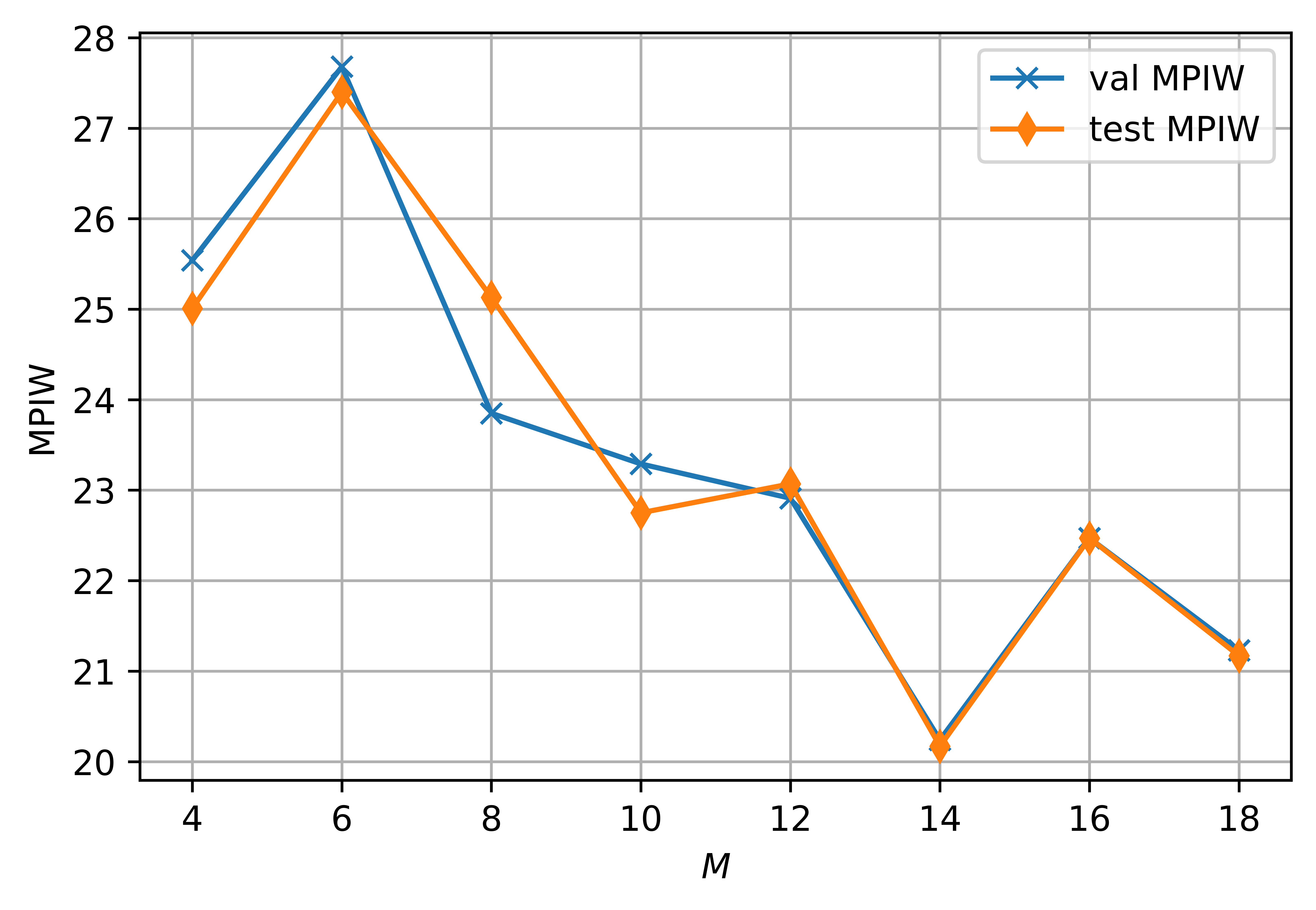
The effectiveness of CDP-ACC largely depends on the accuracy of conditional distribution estimation. In our histogram estimation, the parameter affects this accuracy. A smaller implies a coarser histogram estimation, while a larger results in a finer estimation but reduces the number of sample points within each subinterval , which can also hinder the effectiveness of the approximation. In our experiments, half of the calibration set is used as the validation set for tuning the parameter . As shown in Figs. 7 and 8, the optimal value of the parameter () can be obtained by tuning on the validation set.
V CONCLUSION
By introducing conformal prediction, we propose a plug-and-play uncertainty quantification method CDP to produce confidence intervals for facial depression prediction. The intervals predicted by CDP can achieve marginal coverage guarantee at any given miscoverage rate. Furthermore, we develop CDP-ACC for facial depression prediction. By approximate conditional coverage, it alleviates the issue of marginal coverage practices focusing solely on the average coverage while overlooking individuals with great uncertainty, and provides valid and adaptive confidence intervals for better uncertainty quantification in facial depression prediction. Although our proposed method is used for facial depression prediction, it is also applicable to various other data modalities. We expect that this work will attract more researchers to pay attention to the issue of uncertainty quantification for automated depression prediction in modern context.
To further validate the effectiveness of our CDP-ACC for general regression tasks, we conducted supplementary experiments on seven publicly available datasets, as also used in [45, 52]. These seven datasets are: Physicochemical Properties of Protein Tertiary Structure (bio) [60], BlogFeedback (blog) [61], Facebook Comment Volume Dataset [62], variants one (fb1) and two (fb2), from the UCI Machine Learning Repository [63], and Medical Expenditure Panel Survey (meps19 - meps21) [64]. Regarding the preprocessing of the datasets and the experimental setup, we followed the settings in [45, 52], with detailed information available on GitHub.
Datasets
The Physicochemical Properties of Protein Tertiary Structure (bio) dataset [60] falls under the subject heading of biology. It consists of data extracted from CASP 5-9 and contains 45,730 decoys ranging in size from 0 to 21 angstroms. This dataset is commonly used for multivariate regression analysis.
The BlogFeedback (blog) dataset [61] belongs to the field of social science. It comprises 60,021 instances, each consisting of features extracted from blog posts and a target variable representing the number of comments the post received within 24 hours. This task is a multivariate regression task commonly used to predict the number of comments a post will receive.
The Facebook Comment Volume Dataset (fb1, fb2) [62] is similar to the blog dataset in that it aims to predict the number of comments on a post. It comprises 40,949 instances, each with 53 features. The dataset includes 5 variants; however, we only utilized the first two variants (fb1 and fb2) in our experiment.
The Medical Expenditure Panel Survey (meps 19 - 21) [64] is a series of large-scale surveys conducted on households, individuals, healthcare providers, and employers across the United States. MEPS serves as the most comprehensive data source on healthcare expenses, utilization, and the extent of medical insurance coverage. In our experiments, we exclusively utilized data from panels 19 to 21.
Implementation Details
Our experimental setup follows [45, 52], where we train a conditional quantile estimator (implemented as a three-layer neural network) to handle the regression task described above. We employ the pinball loss (Eq. 4) as our loss function and ensure that the output quantiles are sorted to prevent crossing.
We train the neural network using the Adam optimizer with a learning rate of 0.02. The output quantiles serve as part of the post-processing calibration for conformal prediction. Unlike SCP [26, 44, 27] and CDP-ACC, which do not rely on quantiles, we typically treat the 50% quantile as the output for vanilla regression. We evaluate using Prediction Interval Coverage Probability (PICP) and Mean Prediction Interval Width (MPIW) as metrics, with a miscoverage rate set to 0.1. For specific definitions of these evaluation metrics, please refer to our main paper.
Results
We present the uncertainty quantification results of several methods, including SCP [26, 44, 27], QR [50], CQR [45], CHR [52], and CDP-ACC, on the aforementioned general datasets. QR and CQR are introduced in the main paper. CHR is a histogram estimation method that calibrates the QR method by constructing nested intervals and integrating them with conformal prediction.
From Table V, it is clear that SCP generally achieves marginal coverage but tends to construct unnecessarily conservative intervals. In contrast, in general regression tasks, QR maintains normal coverage rates and effectively reduces the mean interval width (However, in depression prediction task, QR exhibits a trend of overconfidence, with quantile values overly concentrated around predictions, leading to lower coverage rates.)
CQR and CHR serve as calibration methods for QR, aiming to minimize interval width while maintaining adequate coverage rates. However, CQR is constrained by the simplicity of QR in constructing conformal scores. In contrast, CHR integrates histogram estimation with conformal prediction, enabling more refined optimization of prediction intervals.
For QR, CQR, and CHR, retraining the QR model is crucial. However, vanilla regression models with point prediction can only allow for obtaining prediction intervals through post-processing methods like SCP. Nevertheless, SCP has significant drawbacks such as fixed interval width and overly conservative intervals (unnecessarily wide). CDP-ACC, as an adaptive post-processing method, can be applied to both QR and vanilla regression models. It achieves a finer approximation of conditional distributions through binning, thereby further reducing interval width. From Table V, we observe that CDP-ACC achieves competitive uncertainty quantification results, demonstrating its effectiveness on general regression tasks..
| Methods | Data | PICP | MPIW |
| SCP [26, 44, 27] | bio | 90.10% | 14.87 |
| QR [50] | bio | 90.05% | 14.53 |
| CQR [45] | bio | 90.15% | 14.56 |
| CHR [52] | bio | 90.35% | 13.13 |
| CDP-ACC | bio | 89.55% | 12.26 |
| SCP [26, 44, 27] | blog | 91.20% | 16.10 |
| QR [50] | blog | 92.35% | 14.65 |
| CQR [45] | blog | 91.20% | 14.65 |
| CHR [52] | blog | 89.85% | 10.24 |
| CDP-ACC | blog | 90.02% | 9.56 |
| SCP [26, 44, 27] | fb1 | 88.25% | 16.15 |
| QR [50] | fb1 | 92.00% | 15.68 |
| CQR [45] | fb1 | 90.00% | 15.67 |
| CHR [52] | fb1 | 89.60% | 12.23 |
| CDP-ACC | fb1 | 89.15% | 12.11 |
| SCP [26, 44, 27] | fb2 | 90.05% | 18.51 |
| QR [50] | fb2 | 92.55% | 15.44 |
| CQR [45] | fb2 | 89.95% | 15.43 |
| CHR [52] | fb2 | 90.25% | 12.14 |
| CDP-ACC | fb2 | 89.70% | 10.27 |
| SCP [26, 44, 27] | meps19 | 90.05% | 32.55 |
| QR [50] | meps19 | 89.80% | 31.23 |
| CQR [45] | meps19 | 90.95% | 31.37 |
| CHR [52] | meps19 | 90.04% | 22.73 |
| CDP-ACC | meps19 | 89.90% | 17.00 |
| SCP [26, 44, 27] | meps20 | 88.85% | 23.74 |
| QR [50] | meps20 | 88.45% | 26.47 |
| CQR [45] | meps20 | 89.10% | 26.53 |
| CHR [52] | meps20 | 89.35% | 16.56 |
| CDP-ACC | meps20 | 90.05% | 16.00 |
| SCP [26, 44, 27] | meps21 | 90.55% | 26.58 |
| QR [50] | meps21 | 88.80% | 29.91 |
| CQR [45] | meps21 | 90.05% | 29.99 |
| CHR [52] | meps21 | 90.05% | 19.44 |
| CDP-ACC | meps21 | 91.15% | 15.00 |
References
- [1] W. H. Organization et al., “Depression and other common mental disorders: global health estimates,” World Health Organization, Tech. Rep., 2017.
- [2] A. Aprilia and D. Aminatun, “Investigating memory loss: How depression affects students’memory endurance,” Journal of English Language Teaching and Learning, vol. 3, no. 1, pp. 1–11, 2022.
- [3] S. Marwaha, E. Palmer, T. Suppes, E. Cons, A. H. Young, and R. Upthegrove, “Novel and emerging treatments for major depression,” The Lancet, vol. 401, no. 10371, pp. 141–153, 2023.
- [4] S. Bachmann, “Epidemiology of suicide and the psychiatric perspective,” International journal of environmental research and public health, vol. 15, no. 7, p. 1425, 2018.
- [5] B. Singh, T. Olds, R. Curtis, D. Dumuid, R. Virgara, A. Watson, K. Szeto, E. O’Connor, T. Ferguson, E. Eglitis et al., “Effectiveness of physical activity interventions for improving depression, anxiety and distress: an overview of systematic reviews,” British journal of sports medicine, vol. 57, no. 18, pp. 1203–1209, 2023.
- [6] A. T. Beck, R. A. Steer, and G. Brown, “Beck depression inventory–ii,” Psychological assessment, 1996.
- [7] M. Hamilton, “The hamilton rating scale for depression,” in Assessment of depression. Springer, 1986, pp. 143–152.
- [8] K. Kroenke, T. W. Strine, R. L. Spitzer, J. B. Williams, J. T. Berry, and A. H. Mokdad, “The phq-8 as a measure of current depression in the general population,” Journal of affective disorders, vol. 114, no. 1-3, pp. 163–173, 2009.
- [9] C. Shan, S. Gong, and P. W. McOwan, “Facial expression recognition based on local binary patterns: A comprehensive study,” Image and vision Computing, vol. 27, no. 6, pp. 803–816, 2009.
- [10] T. R. Almaev and M. F. Valstar, “Local gabor binary patterns from three orthogonal planes for automatic facial expression recognition,” in 2013 Humaine association conference on affective computing and intelligent interaction. IEEE, 2013, pp. 356–361.
- [11] A. Dhall and R. Goecke, “A temporally piece-wise fisher vector approach for depression analysis,” in 2015 International conference on affective computing and intelligent interaction (ACII). IEEE, 2015, pp. 255–259.
- [12] L. Wen, X. Li, G. Guo, and Y. Zhu, “Automated depression diagnosis based on facial dynamic analysis and sparse coding,” IEEE Transactions on Information Forensics and Security, vol. 10, no. 7, pp. 1432–1441, 2015.
- [13] J. R. Williamson, T. F. Quatieri, B. S. Helfer, G. Ciccarelli, and D. D. Mehta, “Vocal and facial biomarkers of depression based on motor incoordination and timing,” in Proceedings of the 4th international workshop on audio/visual emotion challenge, 2014, pp. 65–72.
- [14] Z. Du, W. Li, D. Huang, and Y. Wang, “Encoding visual behaviors with attentive temporal convolution for depression prediction,” in 2019 14th IEEE international conference on automatic face & gesture recognition (FG 2019). IEEE, 2019, pp. 1–7.
- [15] L. He, M. Niu, P. Tiwari, P. Marttinen, R. Su, J. Jiang, C. Guo, H. Wang, S. Ding, Z. Wang et al., “Deep learning for depression recognition with audiovisual cues: A review,” Information Fusion, vol. 80, pp. 56–86, 2022.
- [16] A. Krizhevsky, I. Sutskever, and G. E. Hinton, “Imagenet classification with deep convolutional neural networks,” Advances in neural information processing systems, vol. 25, 2012.
- [17] W. C. de Melo, E. Granger, and A. Hadid, “A deep multiscale spatiotemporal network for assessing depression from facial dynamics,” IEEE transactions on affective computing, vol. 13, no. 3, pp. 1581–1592, 2020.
- [18] W. C. de Melo, E. Granger, and M. B. Lopez, “Mdn: A deep maximization-differentiation network for spatio-temporal depression detection,” IEEE transactions on affective computing, 2021.
- [19] Y. Zhu, Y. Shang, Z. Shao, and G. Guo, “Automated depression diagnosis based on deep networks to encode facial appearance and dynamics,” IEEE Transactions on Affective Computing, vol. 9, no. 4, pp. 578–584, 2017.
- [20] X. Zhou, Z. Wei, M. Xu, S. Qu, and G. Guo, “Facial depression recognition by deep joint label distribution and metric learning,” IEEE Transactions on Affective Computing, vol. 13, no. 3, pp. 1605–1618, 2022.
- [21] L. He and C. Cao, “Automated depression analysis using convolutional neural networks from speech,” Journal of biomedical informatics, vol. 83, pp. 103–111, 2018.
- [22] Z. Zhao, Q. Li, N. Cummins, B. Liu, H. Wang, J. Tao, and B. Schuller, “Hybrid network feature extraction for depression assessment from speech,” in Proceedings INTERSPEECH 2020. ISCA-INST SPEECH COMMUNICATION ASSOC, 2020, pp. 4956–4960.
- [23] D. Castelvecchi, “Can we open the black box of ai?” Nature News, vol. 538, no. 7623, p. 20, 2016.
- [24] V. Buhrmester, D. Münch, and M. Arens, “Analysis of explainers of black box deep neural networks for computer vision: A survey,” Machine Learning and Knowledge Extraction, vol. 3, no. 4, pp. 966–989, 2021.
- [25] M. Xu, X. Zhang, and X. Zhou, “Confidence-calibrated face and kinship verification,” IEEE Transactions on Information Forensics and Security, 2023.
- [26] V. Vovk, A. Gammerman, and C. Saunders, “Machine-learning applications of algorithmic randomness,” in Proceedings of the Sixteenth International Conference on Machine Learning, 1999, pp. 444–453.
- [27] G. Shafer and V. Vovk, “A tutorial on conformal prediction.” Journal of Machine Learning Research, vol. 9, no. 3, 2008.
- [28] Y. Romano, M. Sesia, and E. Candes, “Classification with valid and adaptive coverage,” Advances in Neural Information Processing Systems, vol. 33, pp. 3581–3591, 2020.
- [29] G. Sharma, A. Parashar, and A. M. Joshi, “Dephnn: a novel hybrid neural network for electroencephalogram (eeg)-based screening of depression,” Biomedical signal processing and control, vol. 66, p. 102393, 2021.
- [30] A. Seal, R. Bajpai, J. Agnihotri, A. Yazidi, E. Herrera-Viedma, and O. Krejcar, “Deprnet: A deep convolution neural network framework for detecting depression using eeg,” IEEE Transactions on Instrumentation and Measurement, vol. 70, pp. 1–13, 2021.
- [31] M. Niu, J. Tao, B. Liu, J. Huang, and Z. Lian, “Multimodal spatiotemporal representation for automatic depression level detection,” IEEE transactions on affective computing, 2020.
- [32] M. A. Uddin, J. B. Joolee, and K.-A. Sohn, “Deep multi-modal network based automated depression severity estimation,” IEEE transactions on affective computing, 2022.
- [33] M. Niu, Y. Li, J. Tao, X. Zhou, and B. W. Schuller, “Depressionmlp: A multi-layer perceptron architecture for automatic depression level prediction via facial keypoints and action units,” IEEE Transactions on Circuits and Systems for Video Technology, 2024.
- [34] W. C. De Melo, E. Granger, and A. Hadid, “Depression detection based on deep distribution learning,” in 2019 IEEE international conference on image processing (ICIP). IEEE, 2019, pp. 4544–4548.
- [35] I. Nouretdinov, S. G. Costafreda, A. Gammerman, A. Chervonenkis, V. Vovk, V. Vapnik, and C. H. Fu, “Machine learning classification with confidence: application of transductive conformal predictors to mri-based diagnostic and prognostic markers in depression,” Neuroimage, vol. 56, no. 2, pp. 809–813, 2011.
- [36] R. Harper and J. Southern, “A bayesian deep learning framework for end-to-end prediction of emotion from heartbeat,” IEEE transactions on affective computing, vol. 13, no. 2, pp. 985–991, 2020.
- [37] N. R. Prabhu, N. Lehmann-Willenbrock, and T. Gerkmann, “End-to-end label uncertainty modeling in speech emotion recognition using bayesian neural networks and label distribution learning,” IEEE Transactions on Affective Computing, 2023.
- [38] W. Wu, C. Zhang, and P. Woodland, “Estimating the uncertainty in emotion attributes using deep evidential regression,” in Proceedings of the 61st Annual Meeting of the Association for Computational Linguistics (Volume 1: Long Papers), 2023, pp. 15 681–15 695.
- [39] L. Lo, B.-K. Ruan, H.-H. Shuai, and W.-H. Cheng, “Modeling uncertainty for low-resolution facial expression recognition,” IEEE transactions on affective computing, 2023.
- [40] J. She, Y. Hu, H. Shi, J. Wang, Q. Shen, and T. Mei, “Dive into ambiguity: Latent distribution mining and pairwise uncertainty estimation for facial expression recognition,” in Proceedings of the IEEE/CVF conference on computer vision and pattern recognition, 2021, pp. 6248–6257.
- [41] N. Le, K. Nguyen, Q. Tran, E. Tjiputra, B. Le, and A. Nguyen, “Uncertainty-aware label distribution learning for facial expression recognition,” in Proceedings of the IEEE/CVF Winter Conference on Applications of Computer Vision, 2023, pp. 6088–6097.
- [42] M. K. Tellamekala, T. Giesbrecht, and M. Valstar, “Dimensional affect uncertainty modelling for apparent personality recognition,” IEEE Transactions on Affective Computing, vol. 13, no. 4, pp. 2144–2155, 2022.
- [43] M. K. Tellamekala, S. Amiriparian, B. W. Schuller, E. André, T. Giesbrecht, and M. Valstar, “Cold fusion: Calibrated and ordinal latent distribution fusion for uncertainty-aware multimodal emotion recognition,” IEEE Transactions on Pattern Analysis and Machine Intelligence, 2023.
- [44] V. Vovk, “Conditional validity of inductive conformal predictors,” in Asian conference on machine learning. PMLR, 2012, pp. 475–490.
- [45] Y. Romano, E. Patterson, and E. Candes, “Conformalized quantile regression,” Advances in neural information processing systems, vol. 32, 2019.
- [46] A. N. Angelopoulos and S. Bates, “A gentle introduction to conformal prediction and distribution-free uncertainty quantification,” arXiv preprint arXiv:2107.07511, 2021.
- [47] P. Cui, W. Hu, and J. Zhu, “Calibrated reliable regression using maximum mean discrepancy,” Advances in Neural Information Processing Systems, vol. 33, pp. 17 164–17 175, 2020.
- [48] M. Valstar, B. Schuller, K. Smith, F. Eyben, B. Jiang, S. Bilakhia, S. Schnieder, R. Cowie, and M. Pantic, “Avec 2013: the continuous audio/visual emotion and depression recognition challenge,” in Proceedings of the 3rd ACM international workshop on Audio/visual emotion challenge, 2013, pp. 3–10.
- [49] M. Valstar, B. Schuller, K. Smith, T. Almaev, F. Eyben, J. Krajewski, R. Cowie, and M. Pantic, “Avec 2014: 3d dimensional affect and depression recognition challenge,” in Proceedings of the 4th international workshop on audio/visual emotion challenge, 2014, pp. 3–10.
- [50] J. W. Taylor, “A quantile regression neural network approach to estimating the conditional density of multiperiod returns,” Journal of forecasting, vol. 19, no. 4, pp. 299–311, 2000.
- [51] N. Tagasovska and D. Lopez-Paz, “Single-model uncertainties for deep learning,” Advances in neural information processing systems, vol. 32, 2019.
- [52] M. Sesia and Y. Romano, “Conformal prediction using conditional histograms,” Advances in Neural Information Processing Systems, vol. 34, pp. 6304–6315, 2021.
- [53] C. Lu, A. N. Angelopoulos, and S. Pomerantz, “Improving trustworthiness of ai disease severity rating in medical imaging with ordinal conformal prediction sets,” in International Conference on Medical Image Computing and Computer-Assisted Intervention. Springer, 2022, pp. 545–554.
- [54] Y. Chung, W. Neiswanger, I. Char, and J. Schneider, “Beyond pinball loss: Quantile methods for calibrated uncertainty quantification,” Advances in Neural Information Processing Systems, vol. 34, pp. 10 971–10 984, 2021.
- [55] R. F. Barber, E. J. Candes, A. Ramdas, and R. J. Tibshirani, “Predictive inference with the jackknife+,” 2021.
- [56] T. Baltrušaitis, P. Robinson, and L.-P. Morency, “Openface: an open source facial behavior analysis toolkit,” in 2016 IEEE winter conference on applications of computer vision (WACV). IEEE, 2016, pp. 1–10.
- [57] D. Tran, L. Bourdev, R. Fergus, L. Torresani, and M. Paluri, “Learning spatiotemporal features with 3d convolutional networks,” in Proceedings of the IEEE international conference on computer vision, 2015, pp. 4489–4497.
- [58] C. Feichtenhofer, H. Fan, J. Malik, and K. He, “Slowfast networks for video recognition,” in Proceedings of the IEEE/CVF international conference on computer vision, 2019, pp. 6202–6211.
- [59] A. N. Angelopoulos, S. Bates, M. Jordan, and J. Malik, “Uncertainty sets for image classifiers using conformal prediction,” in International Conference on Learning Representations.
- [60] P. Rana, “Physicochemical Properties of Protein Tertiary Structure,” UCI Machine Learning Repository, 2013, DOI: https://doi.org/10.24432/C5QW3H.
- [61] K. Buza, “BlogFeedback,” UCI Machine Learning Repository, 2014, DOI: https://doi.org/10.24432/C58S3F.
- [62] K. Singh, “Facebook Comment Volume Dataset,” UCI Machine Learning Repository, 2016, DOI: https://doi.org/10.24432/C5Q886.
- [63] A. Asuncion and D. Newman, “Uci machine learning repository,” 2007.
- [64] J. W. Cohen, S. B. Cohen, and J. S. Banthin, “The medical expenditure panel survey: a national information resource to support healthcare cost research and inform policy and practice,” Medical care, vol. 47, no. 7_Supplement_1, pp. S44–S50, 2009.
![[Uncaptioned image]](https://cdn.awesomepapers.org/papers/a542a549-be3a-4929-9904-b4c5aa60a1a2/yourphoto.jpeg) |
Yonghong Li received a Bachelor of Engineering degree from Chang’an University, Shannxi, China, in 2020. He is currently pursuing his PhD degree at Beijing University of Posts and Telecommunications in Beijing, China, with a focus on affective computing and deep learning. |
![[Uncaptioned image]](https://cdn.awesomepapers.org/papers/a542a549-be3a-4929-9904-b4c5aa60a1a2/Zhou.jpeg) |
Xiuzhuang Zhou (Member, IEEE) received the PhD degree from the School of Computer Science, Beijing Institute of Technology, China, in 2011. He is currently a full professor at the Beijing University of Posts and Telecommunications, Beijing, China. His research interests include computer vision, pattern recognition, multimedia computing, and machine learning. He has authored more than 80 scientific papers in peer reviewed journals and conferences including several top venues such as the IEEE Transactions on Pattern Analysis and Machine Intelligence, CVPR. He serves as an associate editor for the Neurocomputing. |