Conformal covariance of connection probabilities
in the 2D critical FK-Ising model

Fortuin and Kasteleyn introduced the random-cluster model in the 1970s (see [FK72]) as a general family of discrete percolation models that combines together Bernoulli percolation, graphical representations of spin models (Ising & Potts models), and polymer models (as a limiting case). Generally, in such models, edges are declared open or closed according to a given probability measure, the simplest being the independent product measure of Bernoulli percolation. Of particular interest are percolation properties, that is, whether various points in space are connected by paths of open edges.

The random-cluster model has been actively investigated in the past decades, for instance, because of its important feature of criticality: for certain parameter values the model exhibits a continuous phase transition. Criticality can be practically identified as follows. On a lattice with a small mesh, say $\delta\mathbb{Z}^{2}$, consider the probability that an open path connects two opposite sides of a topological rectangle (i.e., a bounded domain with four marked points on its boundary). This probability tends to zero as $\delta\to 0$ when the model is “subcritical,” while it tends to one as $\delta\to 0$ when the model is “supercritical.” At the critical point, the connection probability has a nontrivial limit, which belongs to $(0,1)$ and depends on the “shape” (i.e., the conformal modulus) of the topological rectangle. The exact identification of the limit of the connection probability, though, is highly nontrivial.

The phase transition in the random-cluster model has been argued to result in conformal invariance and universality for the scaling limit of the model (see, e.g., [Car96]). For generic values of the cluster weight parameter $q\in[1,4]$, it was recently shown [DCKK⁺20] that correlations in the critical random-cluster model become rotationally invariant in the scaling limit. This provides strong evidence of conformal invariance, while still not being enough to prove it. Conformal invariance had been previously rigorously established for the FK-Ising model (cluster weight $q=2$) and for Bernoulli site percolation on the triangular lattice (related to Bernoulli bond percolation, corresponding to cluster weight $q=1$) [Smi01, CN06, CN07, Smi10, CS12, CDCH⁺14, KS16, KS19, Izy22].

In addition to proving conformal invariance, identifying in the scaling limit objects that have a conformal field theory (CFT) interpretation is crucial in order to get access to the full power of the CFT formalism applicable to critical lattice models (see, e.g., [Hen13]). In this direction, in the case of critical site percolation on the triangular lattice, one of us recently established [Cam24a, Cam24b] the conformal covariance of connection probabilities in the scaling limit, showing that they can be interpreted as CFT correlations functions and proving a conjecture formalized by Aizenman in the 1990s. We then moved one step forward and started to explore the CFT structure of critical percolation [CF24a, CF24b], identifying the scaling limits of various connection probabilities with CFT correlation functions and proving a rigorous version of an operator product expansion (OPE).

The first main motivation of this article is to provide a natural extension of the aforementioned works [Cam24a, Cam24b] to the FK-Ising model, which is of great interest to both mathematicians and physicists. In those works, the local independence of percolation is used in the proofs, so it is natural to ask whether one can adapt the arguments developed for percolation to deal with the critical random-cluster model with cluster weight $q\neq 1$. In this paper, we focus on the case $q=2$, the only one for which the conformal invariance of the scaling limit of interfaces has been proved so far. As we will see, extending the results of [Cam24a, Cam24b] to the FK model with $q=2$ requires additional work and involves new ingredients, namely a classical result by Wu [MW73] on Ising two-point functions, a spatial mixing property and, in the case of connection probabilities involving boundary points, Smirnov’s FK-Ising fermionic observable (see [Smi10])¹¹1Wu’s result on the Ising two-point function and Smirnov’s FK-Ising observable are only used to figure out the exact orders of the normalization factors in Theorems 1.1 and 1.4..

The second main motivation is to provide an alternative approach to study the conformal covariance and the CFT structure of spin and energy correlations in the Ising and Potts models, which are classical models of ferromagnetism and are among the most studied models of statistical mechanics. In the case of the Ising model, the conformal covariance and the CFT structure of spin and energy correlations have been established rigorously to a large extent [HS13, CI13, CHI15, CHI21, CIM23] using discrete complex analysis tools, where the s-holomorphicity of certain observables plays an essential role. However, s-holomorphicity is difficult to prove beyond the cases of the Ising and FK-Ising models. Since the correlations of some of the most basic Ising and Potts fields, such as the spin and energy fields, can be expressed in terms of point-to-point connection probabilities in the random-cluster model via the Edwards-Sokal coupling²²2In particular, the FK-Ising random-cluster model is related to the Ising spin model. [ES88], it is interesting to develop a geometric approach to study conformal covariance and the CFT structure of spin and energy correlations based on connection probabilities and interfaces in the random-cluster model.³³3It would also be interesting to construct spin or energy correlations directly for $\mathrm{CLE}$ in the continuum. Such an approach is already interesting for the case of the Ising model, but could prove potentially even more useful to study the scaling limits of Potts model with values of $q\neq 2$.

We will show that, for the 2D critical FK-Ising model, (normalized) point-to-point connection probabilities of various kinds of link patterns have conformally covariant scaling limits (see Theorems 1.1 and 1.4 below). As a corollary, we provide a new proof of conformal covariance of Ising spin correlations (see Corollary 2.4 below). The main inputs of the proofs are the FKG inequality, RSW estimates, the one-arm exponent for $\mathrm{CLE}$ computed in [SSW09], and the convergence of interfaces towards $\mathrm{CLE}_{16/3}$ in the Camia-Newman topology⁴⁴4See [CN06]. [KS16, KS19]. We also use a spatial mixing property, which is essentially a consequence of the FKG inequality and RSW estimates, as shown in [DCHN11]. We note that, although [DCHN11] deals with FK percolation with $q=2$, there seems to be no fundamental obstacle to extending the arguments in that paper to other values of $q\in[1,4]$.

In the present paper, results proved using discrete complex analysis techniques are needed directly only when dealing with correlation functions involving boundary vertices, namely in Section 4⁵⁵5In Section 4, they are used to replace a classical result by Wu on Ising correlations between pairs of points in the bulk. and in the appendix. They are also used indirectly because the proofs of convergence of discrete interfaces towards $\mathrm{CLE}_{16/3}$ involve the s-holomorphicity of certain observables (see [KS16, KS19]). However, the recent groundbreaking work [DCKK⁺20] suggests that a proof of convergence and conformal invariance of interfaces for $q\in[1,4]$ without using s-holomorphicity may be possible in the future.

We emphasize that, for our results involving only vertices in the bulk, the convergence of interfaces to $\mathrm{CLE}_{16/3}$ is the only place where s-holomorphicity is used. If one could prove convergence to $\mathrm{CLE}_{\kappa}$ for other FK models with $q\in[1,4]$, then a combination of our arguments in this paper and standard percolation techniques would allow us to extend our results to those FK models, at least in a weaker form (normalizing connection probabilities with the probability of the one-arm event).

For definiteness, we consider subgraphs of the square lattice $\mathbb{Z}^{2}$, which is the graph with vertex set $V(\mathbb{Z}^{2}):=\{z=(m,n)\colon m,n\in\mathbb{Z}\}$ and edge set $E(\mathbb{Z}^{2})$ given by edges $\langle z,w\rangle$ between vertices $z,w\in V(\mathbb{Z}^{2})$ whose Euclidean distance equals one (called neighbors). This is our primal lattice. Its standard dual lattice is denoted by $(\mathbb{Z}^{2})^{\bullet}$. The medial lattice $(\mathbb{Z}^{2})^{\diamond}$ is the graph whose vertices are the centers of the edges of the square lattice and whose edges connect vertices at distance $1/\sqrt{2}$. For a subgraph $G\subset\mathbb{Z}^{2}$, we define its boundary to be the following set of vertices:

$\displaystyle\partial G=\{z\in V(G)\,\colon\,\exists\;w\not\in V(G)\text{ such that }\langle z,w\rangle\in E(\mathbb{Z}^{2})\},$

and similarly for subgraphs of $(\mathbb{Z}^{2})^{\bullet}$ and $(\mathbb{Z}^{2})^{\diamond}$. When we add the subscript or superscript $a$, we mean that the lattices $\mathbb{Z}^{2},(\mathbb{Z}^{2})^{\bullet},(\mathbb{Z}^{2})^{\diamond}$ have been scaled by $a>0$. We consider the models in the scaling limit $a\to 0$. For $z\in\mathbb{C}$ and $r>0$, we write

$$B_{r}(z)=\{w\in\mathbb{C}:|z-w|<r\}.$$

Let $G=(V(G),E(G))$ be a finite subgraph of $\mathbb{Z}^{2}$. A random-cluster configuration $\omega=(\omega_{e})_{e\in E(G)}$ is an element of $\{0,1\}^{E(G)}$. An edge $e\in E(G)$ is said to be open (resp. closed) if $\omega_{e}=1$ (resp. $\omega_{e}=0$). We view the configuration $\omega$ as a subgraph of $G$ with vertex set $V(G)$ and edge set $\{e\in E(G)\colon\omega_{e}=1\}$. We denote by $o(\omega)$ (resp. $c(\omega)$) the number of open (resp. closed) edges in $\omega$.

We are interested in the connectivity properties of the graph $\omega$ with various boundary conditions. The maximal connected⁶⁶6Two vertices $z$ and $w$ are said to be connected by $\omega$ if there exists a sequence $\{z_{j}\colon 0\leq j\leq l\}$ of vertices such that $z_{0}=z$, $z_{l}=w$, and each edge $\langle z_{j},z_{j+1}\rangle$ is open in $\omega$ for $0\leq j<l$. components of $\omega$ are called clusters. The boundary conditions encode how the vertices are connected outside of $G$. More precisely, by a boundary condition $\pi$ we refer to a partition $\pi_{1}\sqcup\cdots\sqcup\pi_{m}$ of $\partial G$. Two vertices $z,w\in\partial G$ are said to be wired in $\pi$ if $z,w\in\pi_{j}$ for some $j$. In contrast, free boundary segments comprise vertices that are not wired with any other vertex (so the corresponding part $\pi_{j}$ is a singleton). We denote by $\omega^{\pi}$ the (quotient) graph obtained from the configuration $\omega$ by identifying the wired vertices in $\pi$.

Finally, the random-cluster model on $G$ with edge-weight $p\in[0,1]$, cluster-weight $q>0$, and boundary condition $\pi$, is the probability measure $\smash{\mu^{\pi}_{p,q,G}}$ on the set $\{0,1\}^{E(G)}$ of configurations $\omega$ defined by

$\displaystyle\mu^{\pi}_{p,q,G}[\omega]:=\;$

$\displaystyle\frac{p^{o(\omega)}(1-p)^{c(\omega)}q^{k(\omega^{\pi})}}{\underset{\omega\in\{0,1\}^{E(G)}}{\sum}p^{o(\omega)}(1-p)^{c(\omega)}q^{k(\omega^{\pi})}},$

where $k(\omega^{\pi})$ is the number of connected components of the graph $\omega^{\pi}$. For $q=2$, this model is also known as the FK-Ising model, while for $q=1$, it is simply the Bernoulli bond percolation (i.e., it is a product measure, with the edges taking independent values). The random-cluster model combines together several important models in the same family. For integer values of $q$, it is very closely related to the $q$-state Potts model, and by taking a suitable limit, the case of $q=0$ corresponds to the uniform spanning tree (see, e.g., [DC20]). For $q\in[1,4]$, it was proven [DCST17] that, for a suitable choice of edge-weight $p$, namely

$\displaystyle p=p_{c}(q):=\frac{\sqrt{q}}{1+\sqrt{q}},$

the random-cluster model exhibits a continuous phase transition in the sense that, for $p>p_{c}(q)$, there almost surely exists an infinite cluster, while for $p<p_{c}(q)$, there is no infinite cluster almost surely. Moreover, the limit $p\searrow p_{c}(q)$ is approached in a continuous way. (This is also expected to hold when $q\in(0,1)$, while it is known that the phase transition is discontinuous when $q>4$ [DCGH⁺21].) Therefore, the scaling limit is expected to be conformally invariant for all $q\in[0,4]$. In the present article, we consider point-to-point connection probabilities in the critical FK-Ising model.

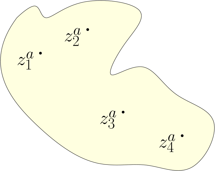
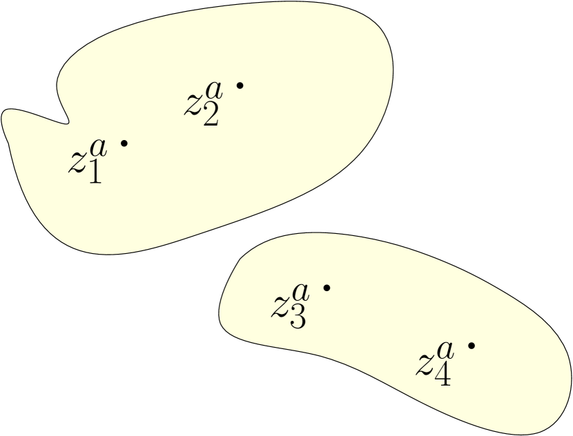
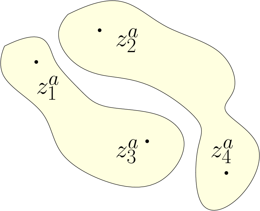
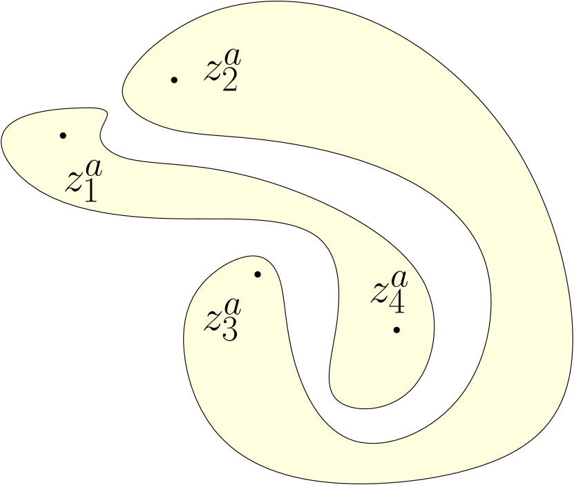
Fix $n\geq 2$, let $\mathbf{Q}=(Q_{1},\ldots,Q_{r})$ be a partition of $\{1,2,\ldots,n\}$. For $a>0$, we denote by $a\mathbb{Z}^{2}$ the scaled square lattice. For a simply connected subgraph $\Omega^{a}\subseteq a\mathbb{Z}^{2}$, we denote by $\mathbb{P}^{a}=\mathbb{P}^{a}_{\Omega}$ the critical FK-Ising measure on $\Omega^{a}$ with free boundary conditions⁷⁷7The boundary condition chosen here is not essential. We can change to, for instance, wired or alternating wired/free boundary conditions.. Let $z_{1}^{a},\ldots,z_{n}^{a}\in\Omega^{a}$ be $n$ distinct vertices. Denote by $G(\mathbf{Q};z_{1}^{a},\ldots,z_{n}^{a})$ the event that $z_{1}^{a},\ldots,z_{n}^{a}$ are connected to each other according to the partition $\mathbf{Q}$, meaning that $z_{i}^{a}$ and $z_{j}^{a}$ are in the same open cluster if and only if $i$ and $j$ are in the same element of $\boldsymbol{Q}$. See Figure 1.1 for a schematic example.

The normalization factor $a^{\frac{1}{8}}$ in (1.1) is related to the interior one-arm exponent for the FK-Ising model and can be derived using Wu’s result on the full-plane Ising two-point spin correlation (see [MW73] and Theorem 2.3 below for more details). As we will see in the proof, without Wu’s result (Theorem 2.3), we can still prove the results in Theorem 1.1 by combining Lemmas 3.3, 3.4 and 3.6 below, but with the normalization factor $a^{\frac{1}{8}}$ replaced by $\mathbb{P}_{\mathbb{Z}^{2}}^{a}[0\longleftrightarrow\partial B_{1}(0)]$.

We emphasize that the domain $\Omega$ in Theorem 1.1 is not necessarily bounded. For $n\geq 2$, we write $\mathbf{Q}_{n}=(\{1,2,\ldots,n\})$ for the special partition with a single element, corresponding to the case in which $z_{1}^{a},\ldots z_{n}^{a}$ belong to the same cluster. Then Theorem 1.1 immediately implies that there exists a constant $C_{1}\in(0,\infty)$ such that

$$P(\mathbb{C};\mathbf{Q}_{2};z_{1},z_{2})=C_{1}|z_{1}-z_{2}|^{-\frac{1}{4}},$$

which can also be derived from the rotational invariance of the full-plane Ising correlations given by [CHI15, Remark 2.26] (or [Pin12]) and the Edwards-Sokal coupling (see [ES88]). Moreover, since Möbius transformations have three degrees of freedom, we can also conclude from Theorem 1.1 that there exists a constant $C_{2}\in(0,\infty)$ such that

$$P(\mathbb{C};\mathbf{Q}_{3};z_{1},z_{2},z_{3})=C_{2}|z_{1}-z_{2}|^{-\frac{1}{8}}|z_{1}-z_{3}|^{-\frac{1}{8}}|z_{2}-z_{3}|^{-\frac{1}{8}}.$$

(1.3)

Consequently, we have the following factorization formula

$$P(\mathbb{C};\mathbf{Q}_{3};z_{1},z_{2},z_{3})=\frac{C_{2}}{C_{1}^{\frac{3}{2}}}\sqrt{P(\mathbb{C};\mathbf{Q}_{2};z_{1},z_{2})\times P(\mathbb{C};\mathbf{Q}_{2};z_{1},z_{3})\times P(\mathbb{C};\mathbf{Q}_{2};z_{2},z_{3})}.$$

Analogous results are derived in [Cam24a, Section 1.1] for percolation, in which case, one knows the value of the constant $C_{2}/C_{1}^{3/2}$ (see [ACSW24]). According to a private communication with one of the authors of [ACSW24], it seems that one may be able to compute the ratio $C_{2}/C_{1}^{3/2}$ also for the FK-Ising model, using the techniques developed in [ACSW24], which rely on Liouville quantum gravity and the imaginary DOZZ formula.

As another application of Theorem 1.1, we can partially recover results from [CHI15]:

The proof of Theorem 1.1 follows the spirit in [Cam24a], that is, relating connection probabilities of interior vertices to the probabilities of events involving interfaces on the lattice and CLE loops in the continuum, conditional on certain crossing events that have probability $0$ in the continuum. However, compared with the percolation case in [Cam24a], in the present case, one encounters additional difficulties due to the lack of independence of the states (open or closed) of different edges. We deal with this problem using the so-called spatial mixing property proved in [DCHN11], which intuitively reads as follows: given two events $\mathcal{A}_{1}$ and $\mathcal{A}_{2}$ that depend only on the states of edges inside edge sets $E_{1}$ and $E_{2}$, respectively, then $\mathcal{A}_{1}$ and $\mathcal{A}_{2}$ are almost independent when $E_{1}$ is far from $E_{2}$ (see Lemma 3.2 for more details).

We denote by $\overline{\mathbb{P}}^{a}=\overline{\mathbb{P}}^{a}_{\Omega}$ the critical FK-Ising measure on $\Omega^{a}$ with wired boundary conditions. The same strategy can be used to show the following result (an analogous result for percolation is proved in [Cam24b]):

We denote by $\mathbb{E}_{\Omega}^{(a,\mathbf{p})}$ the expectation of the critical Ising measure on $\Omega^{a}$ with $\oplus$ boundary condition. Thanks to the Edwards-Sokal coupling (see [ES88]), we have

$$\mathbb{E}_{\Omega}^{(a,\mathbf{p})}\left[\sigma_{z^{a}}\right]=\overline{\mathbb{P}}_{\Omega}^{a}\left[z^{a}\longleftrightarrow\partial\Omega^{a}\right].$$

(1.6)

Consequently, a combination of Theorem 1.3 and (1.6) gives the scaling limit of the Ising magnetization $\mathbb{E}_{\Omega}^{(a,\mathbf{p})}\left[\sigma_{z^{a}}\right]$ normalized by $a^{-\frac{1}{8}}$, which was derived in [CHI15, Corollary 1.3] using discrete complex analysis techniques, with an explicit constant $C_{3}=2^{\frac{5}{12}}e^{-\frac{3}{2}\zeta^{\prime}(-1)}$, where $\zeta^{\prime}$ denotes the derivative of Riemann’s zeta function.

This section concerns the case in which some (or all) of $z_{1}^{a},\ldots,z_{n}^{a}$ are on the boundary of $\Omega^{a}$. In such a situation, we can derive results similar to those in the previous section, but with different normalization factors for the points on the boundary.

For simplicity, we only consider the critical FK-Ising model on the scaled upper half-plane $a\left(\mathbb{H}\cap\mathbb{Z}^{2}\right)$ with free boundary condition on $\mathbb{R}$. We use $\mathbb{P}_{\mathbb{H}}^{a}$ to denote the corresponding measure.

The normalization factor in (1.7) is related to the boundary one-arm exponent for the FK-Ising model (see [Wu18, Theorems 1 and 2]). As part of the proof of (1.9), we will derive

$$\lim_{a\to 0}a^{-\frac{1}{2}}\mathbb{P}^{a}_{\mathbb{H}}\left[0\longleftrightarrow\partial B_{1}(0)\right]=C_{7}$$

(1.9)

using Smirnov’s FK-Ising fermionic observable (see [Smi10]). We note that, without (1.9), one can still obtain a result like (1.7), but with $a^{\frac{1}{2}}$ replaced by $\mathbb{P}_{\mathbb{H}}^{a}\left[0\longleftrightarrow\partial B_{1}(0)\right]$. This follows from the observation that

$$\lim_{a\to 0}\frac{\mathbb{P}_{\mathbb{H}}^{a}\left[0\longleftrightarrow\partial B_{\epsilon}(0)\right]}{\mathbb{P}_{\mathbb{H}}^{a}\left[0\longleftrightarrow\partial B_{1}(0)\right]}=\epsilon^{-\frac{1}{2}},\quad\forall\epsilon>0,$$

(1.10)

which can be derived using the boundary one-arm exponent obtained in [Wu18, Theorems 1 and 2] and the argument in [GPS13, Proof of Proposition 4.9].

In Section 2, we collect some known results that will be used in the proofs of the main results of the paper. In Section 3, we study the connection probabilities of points in the bulk and prove Theorem 1.1. In Section 4, we study connection probabilities of points that can be either in the bulk or on the boundary, and prove Theorem 1.4. The paper ends with an appendix dedicated to the Ising model in a domain with a boundary, in which we provide explicit formulas for some Ising boundary spin correlations.

Theorems 1.1 and 1.4 consider connection probabilities between points at fixed Euclidean distance from each other, which are related to correlation functions of the Ising spin (magnetization) field. The Ising energy correlations on the lattice can also be expressed in terms of point-to-point connection probabilities in the FK-Ising model via the Edwards-Sokal coupling. It would be interesting if one could give a more geometric approach to establish the conformal covariance of Ising energy correlations, as explained in Section 1.1. A fundamental difference is that, in this case, one would need to consider vertices that are a finite number of lattice spaces apart.

In recent works [CF24a, CF24b] on critical Bernoulli site percolation on the triangular lattice, we studied the asymptotic behavior of certain limiting connection probabilities as two points get close to each, identifying the presence of a logarithmic correction to the leading-order power-law behavior. It would be interesting to extend that analysis to the FK model. However, the arguments and ideas in [CF24a, CF24b] are not sufficient to deal with the critical random-cluster models with $q\neq 1$ (even if we assume the convergence of interfaces towards $\mathrm{CLE}_{\kappa}$) because, when $q\neq 1$, one loses independence and, in particular, one needs to consider the influence of the boundary on the states of edges in the bulk.

In future work, we plan to study the Ising energy field and explore a new proof of conformal covariance of Ising energy correlations at criticality based on the convergence of interfaces in the critical FK-Ising model towards $\mathrm{CLE}_{16/3}$, with the hope that it can be generalized to deal with the Potts model with other values of $q$ (assuming the convergence of interfaces towards $\mathrm{CLE}_{\kappa}$ for the corresponding critical random-cluster model).

We will consider the critical FK-Ising model on $\Omega^{a}$ with two types of boundary conditions:

1. 1.

   free boundary conditions,

2. 2.

   Dobrushin boundary conditions, that is, free on $(x_{2}^{a}x_{1}^{a})$ and wired on $(x_{1}^{a}x_{2}^{a})$.

We note that the first type can be considered a degenerate case of the second, with $x_{1}^{a}=x_{2}^{a}$.

Let $\omega\in\{0,1\}^{E(\Omega^{a})}$ be a configuration of the FK-Ising model on $\Omega^{a}$. For both types of boundary conditions mentioned above, we can draw edge-self-avoiding interfaces on $\Omega^{a,\diamond}$ using the edges of the medial lattice as follows:

• •

  each edge belongs to a unique interface,

• •

  edges are connected in such a way that no interface crosses an open primal edge or open dual edge.

In the case of free boundary conditions, the edges of the medial lattice form a collection $\Gamma^{a}$ of loops that do not cross each other or themselves. In the (non-degenerate) case of Dobrushin boundary conditions, in addition to loops, there is an edge-self-avoiding interface $\gamma^{a}$ connecting the outer corners $w_{1}^{a,\diamond}$ and $w_{2}^{a,\diamond}$ on the medial Dobrushin domain $(\Omega^{a,\diamond};x_{1}^{a,\diamond},x_{2}^{a,\diamond})$. Both $\Gamma^{a}$ and $\gamma^{a}$ have a conformally invariant scaling limit, and we will make use of this fact.

In this section, we specify the topologies used to formulate the convergence of loops and interfaces and the convergence of collections of loops.

First, as in [Cam24a], we define a distance function $\Delta$ on $\mathbb{C}\times\mathbb{C}$ given by

$$\Delta(u,v):=\inf_{\phi}\int_{0}^{a}\frac{|\phi^{\prime}(t)|}{1+|\phi(t)|^{2}}\mathrm{d}t,$$

where the infimum is over all differentiable curves $\phi:[0,1]\to\mathbb{C}$ with $\phi(0)=u$ and $\phi(1)=v$. Note that, if we write $\widehat{\mathbb{C}}:=\mathbb{C}\cup\{\infty\}$ and extend $\Delta$ to be a function on $\widehat{\mathbb{C}}\times\widehat{\mathbb{C}}$, then $\left(\widehat{\mathbb{C}},\Delta\right)$ is compact.

Second, for two planar continuous oriented curves $\gamma_{1},\gamma_{2}:[0,1]\to\mathbb{C}$, we define

$$\mathrm{dist}\left(\gamma_{1},\gamma_{2}\right):=\inf_{\psi,\tilde{\psi}}\sup_{t\in[0,1]}\Delta\left(\gamma_{1}(\psi(t)),\gamma_{2}(\tilde{\psi}(t))\right),$$

(2.1)

where the infimum is taken over all increasing homeomorphisms $\psi,\tilde{\psi}:[0,1]\to[0,1]$.

Third, for two sets of loops, $\Gamma_{1}$ and $\Gamma_{2}$, we define

$$\mathrm{Dist}\left(\Gamma_{1},\Gamma_{2}\right):=\inf\left\{\epsilon>0:\forall\gamma_{1}\in\Gamma_{1},\enspace\exists\gamma_{2}\in\Gamma_{2}\text{ s.t. }\mathrm{dist}(\gamma_{1},\gamma_{2})\leq\epsilon\text{ and vice versa}\right\}.$$

(2.2)

We emphasize that the hypothesis on the convergence of discrete domains is not optimal here, but the present version will be sufficient for our purposes.

Consider the critical Ising measure on $a\mathbb{Z}^{2}$ and let $\mathbb{E}_{\mathbb{Z}^{2}}^{a}$ denote the corresponding expectation.

To deal with connection probabilities involving boundary vertices, Theorem 2.3, which is a main ingredient in the proof of Theorem 1.1, is not sufficient. A manifestation of this fact is that the boundary arm exponents are typically different than the interior ones. This affects the normalization of crossing probabilities involving boundary vertices. For this case, unable to use Theorem 2.3, we will find the exact order of the proper normalization using Smirnov’s FK-Ising fermionic observable (see [Smi10]), as explained below.

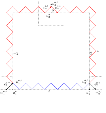
Let $\Box_{2}^{a}=[-2,2]^{2}\cap a\mathbb{Z}^{2}$, consider the the Dobrushin domain $(\Box_{2}^{a};u_{1}^{a},u_{2}^{a})$ and recall the definitions of the medial vertices $u_{1}^{a,\diamond}$ and $u_{2}^{a,\diamond}$ adjacent to $u_{1}^{a}$ and $u_{2}^{a}$ and of the outer corners $w_{1}^{a,\diamond}$ and $w_{2}^{a,\diamond}$ adjacent to $u_{1}^{a,\diamond}$ and $u_{2}^{a,\diamond}$, respectively (see Figure 2.1).

Note that (2.5) gives the sharpness of the boundary one-arm exponent for the FK-Ising model.

The proof of Proposition 2.5 relies on the following observations: (1) the choice of Dobrushin boundary conditions implies that the edges of the medial lattice form a collection $\Gamma^{a}$ of non-crossing loops and an edge-self-avoiding interface $\gamma^{a}$ parameterized from $w_{1}^{a,\diamond}$ to $w_{2}^{a,\diamond}$; (2) denoting by $u_{3}^{a,\diamond}\in\partial\Box_{2}^{a,\diamond}$ the medial vertex to the north of $u_{3}^{a}$ closest to $u_{3}^{a}$ and letting $e_{3,-}^{a,\diamond},e_{3,+}^{a,\diamond}$ be the oriented¹⁰¹⁰10Recall that medial edges are oriented in such a way that the four edges around a vertex of $\mathbb{Z}^{2}$ (respectively, $(\mathbb{Z}^{2})^{\bullet}$) form a circuit that winds around the vertex clockwise (resp., counterclockwise). medial edges around $u_{3}^{a}$ with $u_{3}^{a,\diamond}$ as their end vertex and beginning vertex, respectively (see Figure 2.1), then

$$\{u_{3}^{a}\longleftrightarrow(u_{1}^{a}u_{2}^{a})\}=\{\gamma^{a}\text{ passes through }e_{3,-}^{a,\diamond}\}=\{\gamma^{a}\text{ passes through }e_{3,+}^{a,\diamond}\};$$

(2.6)

(3) the probabilities of the latter two events in (2.6) can be related to the value of Smirnov’s observable on the medial vertex $u_{3}^{a,\diamond}$.

We interpret each oriented medial edge $e^{\diamond}$ as a complex number and define

$$\nu\left(e^{\diamond}\right):=\left(\frac{e^{\diamond}}{|e^{\diamond}|}\right)^{-\frac{1}{2}}.$$

Note that $\nu(e^{\diamond})$ is defined up to a sign, which we will specify when necessary. We denote by $\mathbb{E}_{*}^{a}$ the expectation corresponding to $\mathbb{P}_{*}^{a}$. Now let us recall the definition of FK-Ising fermionic observable given in [Smi10]. Recall that in the Dobrushin domain $(\Box_{2}^{a};u_{1}^{a},u_{2}^{a})$, the outer corner $w_{2}^{a,\diamond}\in(a\mathbb{Z}^{2})^{\diamond}\setminus\Box_{2}^{a,\diamond}$ is a medial vertex adjacent to $u_{2}^{a,\diamond}$, and the outer corner edge $e_{2}^{a,\diamond}$ is the medial edge connecting $u_{2}^{a,\diamond}$ and $w_{2}^{a,\diamond}$.

• •

  First, define the edge observable on edges and outer corner edges $e$ of $\Box_{2}^{a,\diamond}$ as

  $\displaystyle F^{a}(e):=\nu(e_{2}^{a,\diamond})\;\mathbb{E}^{a}_{*}\Big{[}\mathbb{1}\{e\in\gamma^{a}\}\exp\Big{(}-\frac{\mathfrak{i}}{2}W_{\gamma^{a}}\big{(}e_{2}^{\delta,a},e\big{)}\Big{)}\Big{]},$

  where $e_{2}^{a,\diamond}$ is the oriented outer corner edge connecting to $w_{2}^{a,\diamond}$ and oriented to have $w_{2}^{a,\diamond}$ as its end vertex, $W_{\gamma^{a}}\big{(}e_{2}^{a,\diamond},e\big{)}{\in\mathbb{R}}$ is the winding number from $w_{2}^{a,\diamond}$ to $e$ along the reversal of $\gamma^{a}$. Note that $F^{a}$ is only defined up to a sign.

• •

  Second, we define the vertex observable on interior vertices $z^{\diamond}$ of $\Box_{2}^{a,\diamond}$ as

  $\displaystyle F^{a}(z^{\diamond}):=\frac{1}{2}\sum_{e^{\diamond}\sim z^{\diamond}}F^{a}(e^{\diamond}),$

  where the sum is over the four medial edges $e^{\diamond}\sim z^{\diamond}$ having $z^{\diamond}$ as an endpoint.

• •

  Third, we define the vertex observable on vertices in $\partial\Box_{2}^{a,\diamond}\setminus\{u_{1}^{a,\diamond},u_{2}^{a,\diamond}\}$ as follows. For any $z^{a,\diamond}\in\partial\Box_{2}^{a,\diamond}\setminus\{u_{1}^{a,\diamond},u_{2}^{a,\diamond}\}$, let $e_{-}^{a,\diamond},e_{+}^{a,\diamond}\in\partial\Box_{2}^{a,\diamond}\setminus\{u_{1}^{a,\diamond},u_{2}^{a,\diamond}\}$ be the oriented medial edges having $z^{a,\diamond}$ as their end vertex and beginning vertex, respectively. Set

  $\displaystyle F^{a}(z^{\diamond})=\begin{cases}\sqrt{2}\exp(-\mathfrak{i}\frac{\pi}{4})F^{a}(e_{+}^{a,\diamond})+\sqrt{2}\exp(\mathfrak{i}\frac{\pi}{4})F^{a}(e_{-}^{a,\diamond}),&\text{if $z^{a,\diamond}$ $\in(u_{1}^{a,\diamond}u_{2}^{a,\diamond})$},\\[5.0pt] \sqrt{2}\exp(-\mathfrak{i}\frac{\pi}{4})F^{a}(e_{-}^{a,\diamond})+\sqrt{2}\exp(\mathfrak{i}\frac{\pi}{4})F^{a}(e_{+}^{a,\diamond}),&\text{if $z^{a,\diamond}$ $\in(u_{2}^{a,\diamond}u_{1}^{a,\diamond})$}.\end{cases}$

It is a celebrated result in [Smi10] that, as $a\to 0$, the function $2^{-1/4}a^{-\frac{1}{2}}F^{a}(\cdot)$ converges locally uniformly towards an explicit holomorphic function on $[-2,2]^{2}$. Since the boundary of our discrete domain $\Box_{2}^{a}$ is flat near $u_{3}^{a}$, we also have the convergence of $2^{-1/4}a^{-\frac{1}{2}}F^{a}(u_{3}^{a,\diamond})$.

References

- [ACSW24] Morris Ang, Gefei Cai, Xin Sun, and Baojun Wu. Integrability of Conformal Loop Ensemble: Imaginary DOZZ Formula and Beyond. Preprint in arXiv:2107.01788, 2024.
- [ADCTW19] Michael Aizenman, Hugo Duminil-Copin, Vincent Tassion, and Simone Warzel. Emergent planarity in two-dimensional Ising models with finite-range interactions. Invent. Math., 216(3):661–743, 2019.
- [BK89] R. M. Burton and M. Keane. Density and uniqueness in percolation. Comm. Math. Phys., 121(3):501–505, 1989.
- [BPZ84a] A. A. Belavin, A. M. Polyakov, and A. B. Zamolodchikov. Infinite conformal symmetry in two-dimensional quantum field theory. Nuclear Phys. B, 241(2):333–380, 1984.
- [BPZ84b] A. A. Belavin, A. M. Polyakov, and A. B. Zamolodchikov. Infinite conformal symmetry of critical fluctuations in two dimensions. J. Statist. Phys., 34(5-6):763–774, 1984.
- [Cam24a] Federico Camia. Conformal covariance of connection probabilities and fields in 2D critical percolation. Comm. Pure Appl. Math., 77(3):2138–2176, 2024.
- [Cam24b] Federico Camia. On the density of 2D critical percolation gaskets and anchored clusters. Lett. Math. Phys., 114:45, 2024.
- [Car96] John L. Cardy. Scaling and renormalization in statistical physics, volume 5 of Cambridge Lecture Notes in Physics. Cambridge University Press, 1996.
- [CDCH+14] Dmitry Chelkak, Hugo Duminil-Copin, Clément Hongler, Antti Kemppainen, and Stanislav Smirnov. Convergence of Ising interfaces to Schramm’s SLE curves. C. R. Math. Acad. Sci. Paris, 352(2):157–161, 2014.
- [CF24a] Federico Camia and Yu Feng. Conformally covariant probabilities, operator product expansions, and logarithmic correlations in two-dimensional critical percolation. Preprint in arXiv:2407.04246, 2024.
- [CF24b] Federico Camia and Yu Feng. Logarithmic correlation functions in 2D critical percolation. J. High Energy Phys., 2024(8):Paper No. 103, 2024.
- [CHI15] Dmitry Chelkak, Clément Hongler, and Konstantin Izyurov. Conformal invariance of spin correlations in the planar Ising model. Ann. of Math. (2), 181(3):1087–1138, 2015.
- [CHI21] Dmitry Chelkak, Clément Hongler, and Konstantin Izyurov. Correlations of primary fields in the critical planar Ising model. Preprint in arXiv:2103.10263, 2021.
- [CI13] Dmitry Chelkak and Konstantin Izyurov. Holomorphic spinor observables in the critical Ising model. Comm. Math. Phys., 322(2):303–332, 2013.
- [CIM23] Dmitry Chelkak, Konstantin Izyurov, and Rémy Mahfouf. Universality of spin correlations in the Ising model on isoradial graphs. Ann. Probab., 51(3):840–898, 2023.
- [CN06] Federico Camia and Charles M. Newman. Two-dimensional critical percolation: the full scaling limit. Comm. Math. Phys., 268(1):1–38, 2006.
- [CN07] Federico Camia and Charles M. Newman. Critical percolation exploration path and : a proof of convergence. Probab. Theory Related Fields, 139(3-4):473–519, 2007.
- [CN09] Federico Camia and Charles M. Newman. Ising (conformal) fields and cluster area measures. Proc. Natl. Acad. Sci. USA, 106(14):5547–5463, 2009.
- [CS12] Dmitry Chelkak and Stanislav Smirnov. Universality in the 2D Ising model and conformal invariance of fermionic observables. Invent. Math., 189(3):515–580, 2012.
- [DC20] Hugo Duminil-Copin. Lectures on the Ising and Potts models on the hypercubic lattice. In Random graphs, phase transitions, and the Gaussian free field, volume 304 of Springer Proc. Math. Stat., pages 35–161. Springer, Cham, [2020] ©2020.
- [DCGH+21] Hugo Duminil-Copin, Maxime Gagnebin, Matan Harel, Ioan Manolescu, and Vincent Tassion. Discontinuity of the phase transition for the planar random-cluster and Potts models with . Ann. Sci. Éc. Norm. Supér. (4), 54(6):1363–1413, 2021.
- [DCHN11] Hugo Duminil-Copin, Clément Hongler, and Pierre Nolin. Connection probabilities and RSW-type bounds for the two-dimensional FK Ising model. Comm. Pure Appl. Math., 64(9):1165–1198, 2011.
- [DCKK+20] Hugo Duminil-Copin, Karol Kajetan Kozlowski, Dmitry Krachun, Ioan Manolescu, and Mendes Oulamara. Rotational invariance in critical planar lattice models. Preprint in arXiv:2012.11672, 2020.
- [DCST17] Hugo Duminil-Copin, Vladas Sidoravicius, and Vincent Tassion. Continuity of the phase transition for planar random-cluster and Potts models with . Comm. Math. Phys., 349(1):47–107, 2017.
- [Dub07] Julien Dubédat. Commutation relations for Schramm-Loewner evolutions. Comm. Pure Appl. Math., 60(12):1792–1847, 2007.
- [ES88] Robert G. Edwards and Alan D. Sokal. Generalization of the Fortuin-Kasteleyn-Swendsen-Wang representation and Monte Carlo algorithm. Phys. Rev. D (3), 38(6):2009–2012, 1988.
- [FK72] C.M. Fortuin and P.W. Kasteleyn. On the random-cluster model: I. introduction and relation to other models. Physica, 57(4):536–564, 1972.
- [FPW24] Yu Feng, Eveliina Peltola, and Hao Wu. Connection probabilities of multiple FK-Ising interfaces. Probab. Theory Related Fields, 189(1-2):281–367, 2024.
- [GBK78] J. Groeneveld, R.J. Boel, and P.W. Kasteleyn. Correlation-function identities for general planar Ising systems. Physica A: Statistical Mechanics and its Applications, 93(1):138–154, 1978.
- [GPS13] Christophe Garban, Gábor Pete, and Oded Schramm. Pivotal, cluster, and interface measures for critical planar percolation. J. Amer. Math. Soc., 26(4):939–1024, 2013.
- [Hen13] Malte Henkel. Conformal invariance and critical phenomena. Springer Science & Business Media, 2013.
- [HS13] Clément Hongler and Stanislav Smirnov. The energy density in the planar Ising model. Acta Math., 211(2):191–225, 2013.
- [Izy15] Konstantin Izyurov. Smirnov’s observable for free boundary conditions, interfaces and crossing probabilities. Comm. Math. Phys., 337(1):225–252, 2015.
- [Izy22] Konstantin Izyurov. On multiple SLE for the FK-Ising model. Ann. Probab., 50(2):771–790, 2022.
- [KP16] Kalle Kytölä and Eveliina Peltola. Pure partition functions of multiple SLEs. Comm. Math. Phys., 346(1):237–292, 2016.
- [KS16] Antti Kemppainen and Stanislav Smirnov. Conformal invariance in random cluster models. II. Full scaling limit as a branching SLE. Preprint in arXiv:1609.08527, 2016.
- [KS19] Antti Kemppainen and Stanislav Smirnov. Conformal invariance of boundary touching loops of FK Ising model. Comm. Math. Phys., 369(1):49–98, 2019.
- [Law05] Gregory F. Lawler. Conformally invariant processes in the plane, volume 114 of Mathematical Surveys and Monographs. American Mathematical Society, Providence, RI, 2005.
- [MW73] Barry M. McCoy and Tai Tsun Wu. The Two-Dimensional Ising Model. Harvard University Press, Cambridge, MA and London, England, 1973.
- [Pin12] Haru Pinson. Rotational invariance of the 2d spin-spin correlation function. Comm. Math. Phys., 314(3):807–816, 2012.
- [RS05] Steffen Rohde and Oded Schramm. Basic properties of SLE. Ann. of Math. (2), 161(2):883–924, 2005.
- [Smi01] Stanislav Smirnov. Critical percolation in the plane: conformal invariance, Cardy’s formula, scaling limits. C. R. Acad. Sci. Paris Sér. I Math., 333(3):239–244, 2001.
- [Smi10] Stanislav Smirnov. Conformal invariance in random cluster models. I. Holomorphic fermions in the Ising model. Ann. of Math. (2), 172(2):1435–1467, 2010.
- [SSW09] Oded Schramm, Scott Sheffield, and David B. Wilson. Conformal radii for conformal loop ensembles. Comm. Math. Phys., 288(1):43–53, 2009.
- [Wu66] Tai Tsun Wu. Theory of toeplitz determinants and the spin correlations of the two-dimensional Ising model. I. Phys. Rev., 149:380–401, Sep 1966.
- [Wu18] Hao Wu. Polychromatic arm exponents for the critical planar FK-Ising model. J. Stat. Phys., 170(6):1177–1196, 2018.