Conformal Contextual Robust Optimization

Given a dataset $\mathcal{D}=\{(x^{(1)},y^{(1)}),\ldots(x^{(N)},y^{(N)})\}$ of i.i.d. observations from a distribution $\mathcal{P}(X,Y)$, conformal prediction [4, 55] produces prediction regions with distribution-free theoretical guarantees. A prediction region maps from observations of $X$ to sets of possible values for $Y$ and is said to be marginally valid at the $1-\alpha$ level if $\mathcal{P}_{X,Y}(Y\notin\mathcal{C}(X))\leq\alpha$.

Split conformal is one popular version of conformal prediction. In this approach, marginally calibrated regions $\mathcal{C}$ are designed using a “score function” $s(x,y)$. Intuitively, the score function should have the quality that $s(x,y)$ is smaller when it is more reasonable to guess that $Y=y$ given the observation $X=x$. For example, if one has access to a function $\hat{f}(x)$ which attempts to predict $Y$ from $X$, one might take $s(x,y)=\|\hat{f}(x)-y\|$. The score function is evaluated on each point of a dataset $\mathcal{D_{C}}$ called the “calibration dataset,” yielding $\mathcal{S}=\{s(x^{(j)},y^{(j)})\}_{j=1}^{N_{\mathcal{C}}}$, where $N_{\mathcal{C}}:=|\mathcal{D_{C}}|$. Note that the calibration dataset cannot be used to pick the score function; if data is used to design the score function, it must independent of $\mathcal{D_{C}}$. We then define $\widehat{q}(\alpha)$ as the $\lceil(N_{\mathcal{C}}+1)(1-\alpha)\rceil/N_{\mathcal{C}}$ quantile of $\mathcal{S}$. For any future $x$, the set $\mathcal{C}(x)=\{y\mid s(x,y)\leq\widehat{q}(\alpha)\}$ satisfies $1-\alpha\leq\mathcal{P}(Y\in\mathcal{C}(X))$. This inequality is known as the coverage guarantee, and it arises from the exchangeability of the score of a test point $s(x^{\prime},y^{\prime})$ with $\mathcal{S}$. The coverage guarantee possesses finite-sample properties.

As noted in Vovk’s tutorial [55], while the coverage guarantee holds for any score function, different score functions may lead to more or less informative prediction regions. For example, the score $s(x,y)=1$ leads to the highly uninformative prediction region of all possible values of $Y$. Predictive efficiency is one way to quantify informativeness, defined as the inverse of the expected Lebesgue measure of the prediction region, i.e. $\left(\mathbb{E}[|\mathcal{C}(X)|]\right)^{-1}$ [61, 53]. Methods employing conformal prediction often seek to identify prediction regions that are efficient and calibrated.

The problem of summarizing the distribution of a random vector with points $\Xi:=\{\xi^{(i)}\}_{i=1}^{N}$ arises in many contexts, such as in optimal stratification [16, 17], density estimation [28], and signal quantization [43]. Such points are known as representative points (RPs). Denoting the space of all sets $\widehat{\Xi}$ such that $|\widehat{\Xi}|\leq n$ as $\zeta$, the RPs of a random variable $X$ are

For a comprehensive review of representative points, see [24]. Despite extensive study, no general algorithm exists for the efficient construction of representative points for arbitrary distributions. Typical implementations use clustering algorithms, such as Lloyd’s algorithm, on $\{x^{(i)}\}_{i=1}^{M}\sim\mathcal{P}(X)$.

Predict-then-optimize problems are formulated as

where $w$ are decision variables, $C$ an unknown cost parameter, $x$ observed contextual variables, and $\mathcal{W}$ a compact feasible region. The predict-then-optimize framework is so called as the nominal approach first predicts $\widehat{c}:=f(x)$ and subsequently solves $\min_{w}\widehat{c}^{T}w$. Alternatively, a predictive contextual distribution $\mathcal{P}(C\mid x)$ is assumed, with respect to which the optimization formulation is solved. A full review is presented in [22].

This formulation, however, is inappropriate in risk-sensitive downstream tasks. For this reason, recent works have begun investigating a risk-sensitive variant or “robust” alternative to this traditional formulation, namely by replacing $\mathbb{E}[C^{T}w\mid x]$ with $\max_{\widehat{c}\in\mathcal{U}(x)}\widehat{c}^{T}w$ [46, 14, 58], where $\mathcal{U}(x)$ is constructed to guarantee coverage of $c$, precisely stated in Lemma 3.1.

The proof is deferred to Appendix A. Thus, $1-\alpha$ validity of $\mathcal{U}$ ensures the RO procedure produces a valid bound with probability $1-\alpha$, with more efficient prediction regions resulting in tighter upper bounds.

We assume a conditional generative model $q(C\mid X)$ is learned for this prediction task. For most score functions, the min-max optimization problem of Equation 3 is computationally intractable. Crucially, however, we can consider an extension to the score proposed in [60], which lends itself to a decomposition under which such optimization becomes tractable. For a fixed $K$ and $\{\widehat{c_{k}}\}_{k=1}^{K}\sim q(C\mid x)$, let

We refer to this score as “Generalized Probabilistic Conformal Prediction,” (GPCP) whose validity follows from that of the original PCP framework [60]. We discuss the selection of $K$ in Section 3.4.

We fix $\alpha\in[0,1]$ and take $\mathcal{U}(x)$ to be the $1-\alpha$ prediction region $\mathcal{C}(x)$. Let $\phi(w):=\max_{\widehat{c}\in\mathcal{C}(x)}f(w,\widehat{c})$. It follows that $\phi(w)$ is convex by Danskin’s Theorem by assumption of the convexity of $f$ in $w$. Exact solution of the min-max problem, thus, follows using standard gradient-based optimization techniques on $\phi(w)$. By Danskin’s Theorem, $\nabla_{w}\phi(w)=\nabla_{w}f(w,c^{*})$, where $c^{*}:=\max_{\widehat{c}\in\mathcal{C}(x)}f(w,\widehat{c})$. We follow the standard projected gradient descent optimization scheme, projecting into $\mathcal{W}$ at each iterate, denoted by $\Pi_{\mathcal{W}}$.

Efficient solution of this RO problem, therefore, reduces to being able to efficiently solve the maximization problem over $\mathcal{C}(x)$. While challenging over general nonconvex regions, the GPCP score formulation lends itself to a highly structured prediction region, namely of the form $\mathcal{C}(x)=\bigcup_{k=1}^{K}\mathcal{B}_{\widehat{q}}(\widehat{c}_{k})$ with $\mathcal{B}_{\widehat{q}}$ being a ball of radius $\widehat{q}$, the conformal quantile, under the $d$ metric. This decomposition of $\mathcal{C}(x)$ means the maximum can be efficiently computed by aggregating the maxima over the individual balls:

where the maximum over a ball can be efficiently computed with traditional convex optimization techniques. This procedure is summarized in Algorithm 1. The convergence of this procedure proceeds as follows, whose proof is deferred to Appendix B.

Crucially, the convergence highlighted in Lemma 3.2 reveals that the number of “outer” iterations (i.e. $T$) has no dependence on $K$. This is apparent from the proof, in which the iterate count $T$ hinges upon the Lipschitz constant of $\phi(w)=\max_{k}\max_{\widehat{c}\in\mathcal{B}_{\widehat{q}}(\widehat{c}_{k})}f(w,\widehat{c}):=\max_{k}\phi_{k}(w)$, which critically is $L$-Lipschitz regardless of what $K$ is selected, as each $\phi_{k}(w)$ is $L$-Lipschitz.

We can, thus, solely focus attention on the impact the choice of $K$ has on the “inner” optimization computational cost, namely $\max_{k}\phi_{k}(w)$. This linearly increasing cost with $K$, however, must be juxtaposed with the improved statistical efficiency of such prediction regions. In particular, [60] empirically demonstrated region size generally decreased nonlinearly up to a saturation point as a function of $K$.

Critically, this inflection point can be determined prior to performing the optimization, since doing so only requires access to $q(C\mid X)$ and test samples to estimate the prediction region size. As pointed out in [60] and proven in [13], estimation of the volume of a union of hyperspheres is complicated by the need to account for overlapped regions. $K$ is, thus, chosen based on Monte Carlo estimates of the prediction region volume using Voronoi cells of the hypersphere centers given by [21]:

where $C\sim U(\mathcal{B}_{\widehat{q}}(\widehat{c}_{k}))$ denotes a random variable defined uniformly over the region associated with $\widehat{c}_{k}$, $|\mathcal{B}_{\widehat{q}}|$ the volume of a hypersphere of radius $\widehat{q}$, and $V(\widehat{c}_{k})$ the Voronoi cell of $\widehat{c}_{k}$, defined as $\{z\in\mathbb{R}^{d}\mid d(\widehat{c}_{k},z)\leq d(\widehat{c}_{k^{\prime}},z),k^{\prime}\neq k\}$. Muller’s method enables efficient sampling of $U(\mathcal{B}_{\widehat{q}}(\widehat{c}_{k}))$ [45, 27].

We then choose $K^{*}$ to be the inflection point, namely the $\operatorname*{arg\,min}_{K}|\widehat{\ell}_{K}-\widehat{\ell}_{K+1}|\leq\epsilon$ for some user-specified $\epsilon$ volume tolerance. Critically, these volume estimates must be performed on a distinct subset of the data from $\mathcal{D}_{\mathcal{C}}$ as exchangeability with future test points is otherwise lost in conditioning on $\mathcal{D_{C}}$ for selecting $K^{*}$ [61]. We, thus, partition $\mathcal{D}_{\mathcal{C}}:=\mathcal{D}_{\mathcal{C}_{1}}\cup\mathcal{D}_{\mathcal{C}_{2}}$, using $\mathcal{D}_{\mathcal{C}_{1}}$ for calibration and $\mathcal{D}_{\mathcal{C}_{2}}$ for volume estimation, detailed in Algorithm 2.

We now frame the problem of summarizing the prediction region $\mathcal{C}(x)$. We critically note that this issue of interpretability is non-existent in traditional approaches to robust predict-then-optimize, where uncertainty regions are interpretable by construction, being balls around nominal estimates $\mathcal{B}_{\epsilon}(\widehat{c})$. In other words, there is a fundamental tension in qualitative interpretability and the expressiveness of uncertainty regions, requiring a bespoke method for recovering intuition when leveraging conformal prediction regions. Formally, for a user-specified number of summary points $N$ and query $x$, we seek

We use the shorthand $d(C,\Xi):=\min_{\xi^{(i)}\in\Xi}d(C,\xi^{(i)})$. In other words, we wish to construct representative points for a uniform sampling of the prediction region. A naive approach would simply involve explicitly gridding the output space $\mathcal{C}$, filtering such points with the rejection criterion of $\mathcal{C}(x)$, and clustering the remaining points per the $d$ metric. This, however, is intractable in high-dimensional cases. Thus, a sampling method is employed to circumvent gridding, paralleling the technique leveraged for volume estimation.

$M$ samples are initially drawn $\{c_{k,m}\}_{m=1}^{M}\sim U(\mathcal{B}_{\widehat{q}}(\widehat{c}_{k}))$ for each $k$. Importantly, such uniform sampling of the balls leads to non-uniform sampling over $\mathcal{C}(x)$ if naively aggregated across $k$, as overlapped regions will be more densely sampled. For this reason, we subsample by discarding those samples $c_{k,m}$ for which $c_{k,m}\in V(\widehat{c}_{k^{\prime}})$ for $k\neq k^{\prime}$. This results in samples $C:=\{c_{i}\}$ drawn from the desired $U(\mathcal{C}(x))$.

RPs must be aggregated separately for each connected subregion of $\Omega_{\ell}\subset\mathcal{C}(x)$ to ensure each $\xi^{(i)}\in\mathcal{C}(x)$. That is, we must identify $C_{\ell}:=C\cap\Omega_{\ell}$. To do so, we determine if two points $(c_{i},c_{j})$ belong to the same $\Omega_{\ell}$ by considering the corresponding connected components problem defined on the graph induced by the edge criterion $e_{i,j}=\mathbbm{1}[d(c_{i},c_{j})<\widehat{q}]$. For each $C_{\ell}$, we find a subset $N_{\ell}:=N(|C_{\ell}|/|C|)$ of the total $N$ representative points, for which we use K-Means++ with the $d$ metric. The full procedure is in Algorithm 3.

After obtaining $\Xi$, further insight can be gleaned by exploring the local projection around each $\xi^{(i)}$. An example of this is visualizing the road-level variability in traffic predictions from uncertainty in upstream weather predictions, shown in Figure 5. To do this, we visualize the extent of the Voronoi cell $V^{(i)}\subset\mathcal{C}(x)$ associated with $\xi^{(i)}$ along the $\mathcal{C}$ space dimensions. That is, for each Voronoi cell, we visualize the Frechet variance along the projections $\{\pi_{j}\}_{j=1}^{J}$, where $J=\text{dim}(\mathcal{C})$. Such projections preserve the structure of the objects being modeled, making them visually interpretable. For instance, $\pi_{j}$ in the traffic example corresponds to the projection of $V^{(i)}$ to a single road $j$. Similarly, $\pi_{j}$ would project to a single atom for a molecular reconstruction task. Formally,

We first study the fractional knapsack problem under various complex contextual mappings, namely

where $p\in\mathbb{R}^{n}$ and $B>0$. The distributions $\mathcal{P}(C)$ and $\mathcal{P}(X\mid C)$ are taken to be those from various simulation-based inference (SBI) benchmark tasks provided by [30], chosen as they have $\mathcal{P}(C\mid X)$ with complex structure. We specifically study Two Moons, Lotka-Volterra, Gaussian Linear Uniform, Bernoulli GLM, Susceptible-Infected-Recovered (SIR), and Gaussian Mixture, fully described in Appendix C. We note that, while these particular distributions have little semantic meaning in the traditional context of fractional knapsack, this experiment highlights the capacity for CPO to succeed even for complex distributions, which we leverage in a more semantically meaningful case in Section 4.2.

Optimal routing is a long-standing point of interest in the operations research community, with widespread applications such as in resource distribution and urban traffic flow management [44, 51, 47, 38]. We study the traffic flow problem from [3].

Recent work has demonstrated the utility of generative models in quantifying uncertainty for weather predictions over traditional physics-based approaches [1, 6, 29, 57]. We specifically leverage a latent diffusion model for such forecasting from [39]. Formally, a forecaster $\mathcal{P}(\widetilde{Y}\mid x)$ maps precipitation readings from radar networks $x\in\mathbb{R}^{T\times W\times H}$, specifically over $T$ time steps with resolutions $W\times H$, to $\widetilde{Y}\in\mathbb{R}^{W\times H}$, the precipitation for some fixed $\Delta T$ point beyond $x$.

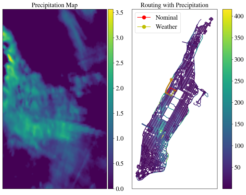
We consider the robust traffic flow problem (RTFP) for a source-target pair $(s,t)$ over the network graph of Manhattan, where $|\mathcal{V}|=4584$ and $|\mathcal{E}|=9867$. The precipitation $\widetilde{Y}$ was combined with the nominal speed limits to obtain the final travel costs $c$ along edges, fully described in Appendix G. Formally, we seek

where $w_{e}$ represents the proportion of traffic routed along edge $e$, $C\in\mathbb{R}^{|\mathcal{E}|}$ is the edge weight vector, $A\in\mathbb{R}^{|\mathcal{V}|\times|\mathcal{E}|}$ is the node-arc incidence matrix, and $b\in\mathbb{R}^{|\mathcal{V}|}$ has entries $b_{s}=1,b_{t}=-1,$ and $b_{k}=0$ for $k\notin\{s,t\}$.

We again demonstrate the quantitative improvement in decision-making resulting from using the more informative CPO prediction regions. Experiments were conducted with $s$ and $t$ chosen uniformly at random from $\mathcal{V}$. We take the score as defined in Equation 12 on the edge weight space rather than the initial precipitation map space. Results are shown in Table 2. Again, although all approaches achieve coverage guarantees, bounds resulting from alternate regions are significantly looser compared to those from CPO. This is especially prominent in this task compared to those of Section 4.1 due to the high dimension of the prediction space($\mathbb{R}^{|\mathcal{E}|}$) and complex nature of $\mathcal{P}(C|X)$.

Notably, the formulation in Equation 14 is a relaxation of the standard LP formulation of the robust shortest paths problem (RSPP), in which $\mathcal{W}=\{0,1\}^{\mathcal{E}}$. Given that $A$ is a totally unimodular matrix, the solutions of the box-constrained RTFP and RSPP are equivalent, i.e. for both Box and PTC-B; they, however, are not equivalent under more general constraint sets [12], i.e. Ellipsoid, PTC-E, and CPO, resulting in the observed suboptimality of box constraints. This is highlighted in Figure 4, where the Box constraint results in a fully concentrated allocation of traffic along a single path.

Despite apparent quantitative improvements resulting from the CPO optimal solution, it is difficult to directly understand why such allocations were deemed optimal without a qualitative impression of $\mathcal{U}(x)$, as framed in Section 3.5. We, therefore, now construct $N=5$ representative points and their corresponding projections, two of which are visualized in Figure 5. The RPs highlight the multimodal nature of the edge weights distribution, where $\xi^{(1)}$ exhibits a case of precipitation more heavily concentrating along the northeast corridor across Manhattan and $\xi^{(2)}$ one where it concentrates on the west. In addition, the projection around $\xi^{(2)}$ reveals especially high uncertainty on the path through Central Park with less on surrounding roads. CPO, thus, hedges its allocation in Figure 4 more evenly across paths, unlike the concentrated allocation under the Box region.

References

- [1] Shreya Agrawal et al. “Machine learning for precipitation nowcasting from radar images” In arXiv preprint arXiv:1912.12132, 2019
- [2] Luca Ambrogioni et al. “Forward amortized inference for likelihood-free variational marginalization” In The 22nd International Conference on Artificial Intelligence and Statistics, 2019, pp. 777–786 PMLR
- [3] Enrico Angelelli, Valentina Morandi, Martin Savelsbergh and Maria Grazia Speranza “System optimal routing of traffic flows with user constraints using linear programming” In European journal of operational research 293.3 Elsevier, 2021, pp. 863–879
- [4] Anastasios N Angelopoulos and Stephen Bates “A gentle introduction to conformal prediction and distribution-free uncertainty quantification” In arXiv preprint arXiv:2107.07511, 2021
- [5] Anastasios N Angelopoulos et al. “Image-to-image regression with distribution-free uncertainty quantification and applications in imaging” In International Conference on Machine Learning, 2022, pp. 717–730 PMLR
- [6] Georgy Ayzel, Tobias Scheffer and Maik Heistermann “RainNet v1. 0: a convolutional neural network for radar-based precipitation nowcasting” In Geoscientific Model Development 13.6 Copernicus GmbH, 2020, pp. 2631–2644
- [7] Omer Belhasin et al. “Principal Uncertainty Quantification with Spatial Correlation for Image Restoration Problems” In arXiv preprint arXiv:2305.10124, 2023
- [8] Aharon Ben-Tal, Laurent El Ghaoui and Arkadi Nemirovski “Robust optimization” Princeton university press, 2009
- [9] Dimitris Bertsimas, Vishal Gupta and Nathan Kallus “Data-driven robust optimization” In Mathematical Programming 167 Springer, 2018, pp. 235–292
- [10] Hans-Georg Beyer and Bernhard Sendhoff “Robust optimization–a comprehensive survey” In Computer methods in applied mechanics and engineering 196.33-34 Elsevier, 2007, pp. 3190–3218
- [11] Geoff Boeing “OSMnx: New methods for acquiring, constructing, analyzing, and visualizing complex street networks” In Computers, Environment and Urban Systems 65 Elsevier, 2017, pp. 126–139
- [12] Diah Chaerani, Cornelis Roos and A Aman “The robust shortest path problem by means of robust linear optimization” In Operations Research Proceedings 2004: Selected Papers of the Annual International Conference of the German Operations Research Society (GOR). Jointly Organized with the Netherlands Society for Operations Research (NGB) Tilburg, September 1–3, 2004, 2005, pp. 335–342 Springer
- [13] Timothy M Chan “A (slightly) faster algorithm for Klee’s measure problem” In Proceedings of the twenty-fourth annual symposium on Computational geometry, 2008, pp. 94–100
- [14] Abhilash Reddy Chenreddy, Nymisha Bandi and Erick Delage “Data-driven conditional robust optimization” In Advances in Neural Information Processing Systems 35, 2022, pp. 9525–9537
- [15] Meysam Cheramin, Richard Li-Yang Chen, Jianqiang Cheng and Ali Pinar “Data-driven robust optimization using scenario-induced uncertainty sets” In arXiv preprint arXiv:2107.04977, 2021
- [16] Tore Dalenius “The problem of optimum stratification” In Scandinavian Actuarial Journal 1950.3-4 Taylor & Francis, 1950, pp. 203–213
- [17] Tore Dalenius and Margaret Gurney “The problem of optimum stratification. II” In Scandinavian Actuarial Journal 1951.1-2 Taylor & Francis, 1951, pp. 133–148
- [18] Finale Doshi-Velez and Been Kim “Towards a rigorous science of interpretable machine learning” In arXiv preprint arXiv:1702.08608, 2017
- [19] Conor Durkan, Artur Bekasov, Iain Murray and George Papamakarios “Neural spline flows” In Advances in Neural Information Processing Systems 32, 2019
- [20] Conor Durkan, Artur Bekasov, Iain Murray and George Papamakarios “nflows: normalizing flows in PyTorch” Zenodo, 2020 DOI: 10.5281/zenodo.4296287
- [21] H. Edelsbrunner “The union of balls and its dual shape” In Discrete & Computational Geometry 13.3, 1995, pp. 415–440 DOI: 10.1007/BF02574053
- [22] Adam N Elmachtoub and Paul Grigas “Smart “predict, then optimize”” In Management Science 68.1 INFORMS, 2022, pp. 9–26
- [23] Adam N Elmachtoub, Jason Cheuk Nam Liang and Ryan McNellis “Decision trees for decision-making under the predict-then-optimize framework” In International Conference on Machine Learning, 2020, pp. 2858–2867 PMLR
- [24] Kai-Tai Fang and Jianxin Pan “A Review of Representative Points of Statistical Distributions and Their Applications” In Mathematics 11.13 MDPI, 2023, pp. 2930
- [25] Clara Fannjiang et al. “Conformal prediction under feedback covariate shift for biomolecular design” In Proceedings of the National Academy of Sciences 119.43 National Acad Sciences, 2022, pp. e2204569119
- [26] Shai Feldman, Stephen Bates and Yaniv Romano “Calibrated multiple-output quantile regression with representation learning” In Journal of Machine Learning Research 24.24, 2023, pp. 1–48
- [27] George Fishman “Monte Carlo: concepts, algorithms, and applications” Springer Science & Business Media, 2013
- [28] Bernard D Flury and Thaddeus Tarpey “Representing a large collection of curves: A case for principal points” In The American Statistician 47.4 Taylor & Francis, 1993, pp. 304–306
- [29] Gabriele Franch et al. “Precipitation nowcasting with orographic enhanced stacked generalization: Improving deep learning predictions on extreme events” In Atmosphere 11.3 MDPI, 2020, pp. 267
- [30] Joeri Hermans et al. “Averting a crisis in simulation-based inference” In arXiv preprint arXiv:2110.06581, 2021
- [31] Eliahu Horwitz and Yedid Hoshen “Conffusion: Confidence intervals for diffusion models” In arXiv preprint arXiv:2211.09795, 2022
- [32] Edward J Hu et al. “GFlowNet-EM for learning compositional latent variable models” In International Conference on Machine Learning, 2023, pp. 13528–13549 PMLR
- [33] Yuge Hu, Joseph Musielewicz, Zachary W Ulissi and Andrew J Medford “Robust and scalable uncertainty estimation with conformal prediction for machine-learned interatomic potentials” In Machine Learning: Science and Technology 3.4 IOP Publishing, 2022, pp. 045028
- [34] Rafael Izbicki, Gilson Shimizu and Rafael B Stern “Cd-split and hpd-split: Efficient conformal regions in high dimensions” In The Journal of Machine Learning Research 23.1 JMLRORG, 2022, pp. 3772–3803
- [35] Chancellor Johnstone and Bruce Cox “Conformal uncertainty sets for robust optimization” In Conformal and Probabilistic Prediction and Applications, 2021, pp. 72–90 PMLR
- [36] Margot E Kaminski “The right to explanation, explained” In Berkeley Technology Law Journal 34.1 JSTOR, 2019, pp. 189–218
- [37] Diederik P Kingma and Jimmy Ba “Adam: A method for stochastic optimization” In arXiv preprint arXiv:1412.6980, 2014
- [38] Václav Kořenář “Vehicle routing problem with stochastic demands” In ALLOCATION FRAGMENTS OF THE DISTRIBUTED DATABASE, 2003, pp. 24
- [39] Jussi Leinonen et al. “Latent diffusion models for generative precipitation nowcasting with accurate uncertainty quantification” In arXiv preprint arXiv:2304.12891, 2023
- [40] Jan-Matthis Lueckmann et al. “Benchmarking simulation-based inference” In International Conference on Artificial Intelligence and Statistics, 2021, pp. 343–351 PMLR
- [41] Nikolay Malkin et al. “GFlowNets and variational inference” In arXiv preprint arXiv:2210.00580, 2022
- [42] Huiying Mao, Ryan Martin and Brian J Reich “Valid model-free spatial prediction” In Journal of the American Statistical Association Taylor & Francis, 2022, pp. 1–11
- [43] Joel Max “Quantizing for minimum distortion” In IRE Transactions on Information Theory 6.1 IEEE, 1960, pp. 7–12
- [44] Andrea Mor and Maria Grazia Speranza “Vehicle routing problems over time: a survey” In Annals of Operations Research 314.1 Springer, 2022, pp. 255–275
- [45] Mervin E Muller “A note on a method for generating points uniformly on n-dimensional spheres” In Communications of the ACM 2.4 ACM New York, NY, USA, 1959, pp. 19–20
- [46] Shunichi Ohmori “A predictive prescription using minimum volume k-nearest neighbor enclosing ellipsoid and robust optimization” In Mathematics 9.2 MDPI, 2021, pp. 119
- [47] Michał Okulewicz and Jacek Mańdziuk “A metaheuristic approach to solve dynamic vehicle routing problem in continuous search space” In Swarm and Evolutionary Computation 48 Elsevier, 2019, pp. 44–61
- [48] Adam Paszke et al. “Pytorch: An imperative style, high-performance deep learning library” In Advances in Neural Information Processing Systems 32, 2019
- [49] Yash Patel et al. “Variational Inference with Coverage Guarantees” In arXiv preprint arXiv:2305.14275, 2023
- [50] Egon Peršak and Miguel F Anjos “Contextual robust optimisation with uncertainty quantification” In International Conference on Integration of Constraint Programming, Artificial Intelligence, and Operations Research, 2023, pp. 124–132 Springer
- [51] Meead Saberi and İ Ömer Verbas “Continuous approximation model for the vehicle routing problem for emissions minimization at the strategic level” In Journal of Transportation Engineering 138.11 American Society of Civil Engineers, 2012, pp. 1368–1376
- [52] Utsav Sadana et al. “A Survey of Contextual Optimization Methods for Decision Making under Uncertainty” In arXiv preprint arXiv:2306.10374, 2023
- [53] Matteo Sesia and Emmanuel J Candès “A comparison of some conformal quantile regression methods” In Stat 9.1 Wiley Online Library, 2020, pp. e261
- [54] Matteo Sesia and Yaniv Romano “Conformal prediction using conditional histograms” In Advances in Neural Information Processing Systems 34, 2021, pp. 6304–6315
- [55] Glenn Shafer and Vladimir Vovk “A Tutorial on Conformal Prediction.” In Journal of Machine Learning Research 9.3, 2008
- [56] Chao Shang and Fengqi You “A data-driven robust optimization approach to scenario-based stochastic model predictive control” In Journal of Process Control 75 Elsevier, 2019, pp. 24–39
- [57] Xingjian Shi et al. “Deep learning for precipitation nowcasting: A benchmark and a new model” In Advances in neural information processing systems 30, 2017
- [58] Chunlin Sun, Linyu Liu and Xiaocheng Li “Predict-then-Calibrate: A New Perspective of Robust Contextual LP” In arXiv preprint arXiv:2305.15686, 2023
- [59] Renukanandan Tumu, Lars Lindemann, Truong Nghiem and Rahul Mangharam “Physics constrained motion prediction with uncertainty quantification” In arXiv preprint arXiv:2302.01060, 2023
- [60] Zhendong Wang et al. “Probabilistic conformal prediction using conditional random samples” In arXiv preprint arXiv:2206.06584, 2022
- [61] Yachong Yang and Arun Kumar Kuchibhotla “Finite-sample efficient conformal prediction” In arXiv preprint arXiv:2104.13871, 2021
Checklist
-
1.
For all models and algorithms presented, check if you include:
(a)
A clear description of the mathematical setting, assumptions, algorithm, and/or model. [Yes]
(b)
An analysis of the properties and complexity (time, space, sample size) of any algorithm. [Yes]
(c)
(Optional) Anonymized source code, with specification of all dependencies, including external libraries. [No, will be released upon acceptance]
2.
For any theoretical claim, check if you include:
Statements of the full set of assumptions of all theoretical results. [Yes]
Complete proofs of all theoretical results. [Yes]
Clear explanations of any assumptions. [Yes]
3.
For all figures and tables that present empirical results, check if you include:
The code, data, and instructions needed to reproduce the main experimental results (either in the supplemental material or as a URL). [Yes]
All the training details (e.g., data splits, hyperparameters, how they were chosen). [Yes]
A clear definition of the specific measure or statistics and error bars (e.g., with respect to the random seed after running experiments multiple times). [Yes]
(d)
A description of the computing infrastructure used. (e.g., type of GPUs, internal cluster, or cloud provider). [Yes]
4.
If you are using existing assets (e.g., code, data, models) or curating/releasing new assets, check if you include:
Citations of the creator If your work uses existing assets. [Not Applicable]
The license information of the assets, if applicable. [Not Applicable]
New assets either in the supplemental material or as a URL, if applicable. [Not Applicable]
Information about consent from data providers/curators. [Not Applicable]
(e)
Discussion of sensible content if applicable, e.g., personally identifiable information or offensive content. [Not Applicable]
5.
If you used crowdsourcing or conducted research with human subjects, check if you include:
The full text of instructions given to participants and screenshots. [Not Applicable]
Descriptions of potential participant risks, with links to Institutional Review Board (IRB) approvals if applicable. [Not Applicable]
The estimated hourly wage paid to participants and the total amount spent on participant compensation. [Not Applicable]
Appendix A Prediction Region Validity Lemma
Lemma A.1.
Consider any that is -Lipschitz in under the metric for any fixed . Assume further that . Then,