Confining potential under the gauge field condensation in the SU(2) Yang-Mills theory
Abstract
potential is studied in the SU(2) gauge theory. Based on the nonlinear gauge of the Curci-Ferrari type, the possibility of a gluon condensation in low-energy region has been considered at the one-loop level. Instead of the magnetic monopole condensation, this condensation makes classical gluons massive, and can yield a linear potential. We show this potential consists of the Coulomb plus linear part and an additional part. Comparing with the Cornell potential, we study this confining potential in detail, and find that the potential has two implicit scales and . The meanings of these scales are clarified. We also show that the Cornell potential that fits well to this confining potential is obtained by taking these scales into account.
B0,B3,B6
1 Introduction
In the study of quarkonia, QCD potential is often used. Although there are some phenomenological potentials (see, e.g., bali ), the Cornell potential cor ; cor2 is simple but workable. This potential has the Coulomb plus linear form as
| (1.1) |
where and , that is called the string tension, are constants. The Coulomb part is expected from the perturbative one-gluon exchange, and the linear part represents the confinement.
Is it possible to derive from QCD? Using the dual Ginzburg-Landau model (see, e.g., rip ), the following Yukawa plus linear potential was obtained suz ; mts ; sst ; sst2 :
| (1.2) |
where is the static quark charge and is the momentum cut-off. In this model, the mass is related to the vacuum expectation value (VEV) of the monopole field. In Ref. hs , based on the SU(2) gauge theory in the non-linear gauge of the Curci-Ferrari type, we also derived the potential . In this case, the mass comes from the gauge field condensation .
In this paper, in the framework of Refs. hs ; hs1 , we restudy the confining potential. In the next section, we briefly review Refs. hs ; hs1 , and present the potential between the static charges and . In Sect. 3, the equation to determine an ultraviolet cut-off is derived. In Sect. 4, using this cut-off, we show that the potential becomes the confining potential , where is the additional potential. The potential has several parameters. Comparing with , and choosing the appropriate values of and , the parameters in are determined in Sect. 5. In this process, we find a scale . In the intermediate region, the scale has been proposed so . The meanings of the scales and for are clarified in Sect. 6. We also propose a scale that is related to . Based on this analysis, we obtain that fits well to . Section 7 is devoted to a summary and comments. In Appendix A, the propagator for the off-diagonal gluons is presented. The equations in Sect. 5, that determine the values of the parameters in , are solved in Appendix B.
2 Condensate and potential
2.1 Ghost condensation
We consider the SU(2) gauge theory in Euclidean space. The Lagrangian in the nonlinear gauge of the Curci-Ferrari type cf is
| (2.1) |
where is the Nakanishi-Lautrup field, () is the ghost (antighost), , and are gauge parameters, and is a constant to keep the BRS symmetry. Introducing the auxiliary field , which represents , is rewritten as hs2
| (2.2) |
In Ref. hs3 , by integrating out and with momentum , we studied the one-loop effective potential for , and showed that acquires the VEV under an energy scale . The scale and the VEV are
| (2.3) |
At the one-loop order, it is shown that is the ultraviolet fixed point, where is the first coefficient of the renormalization group function for SU(2). So, when , the relation
| (2.4) |
holds hs3 , where is the QCD scale parameter.
2.2 Condensate
When , the ghost Lagrangian becomes
| (2.5) |
Because of the term in Eq.(2.5), the two-point function
shows the tachyonic behavior. In fact, the ghost loop depicted in Fig. 1(b) yields the tachyonic mass for in the low momentum limit . In the same way, has the tachyonic mass in this limit.
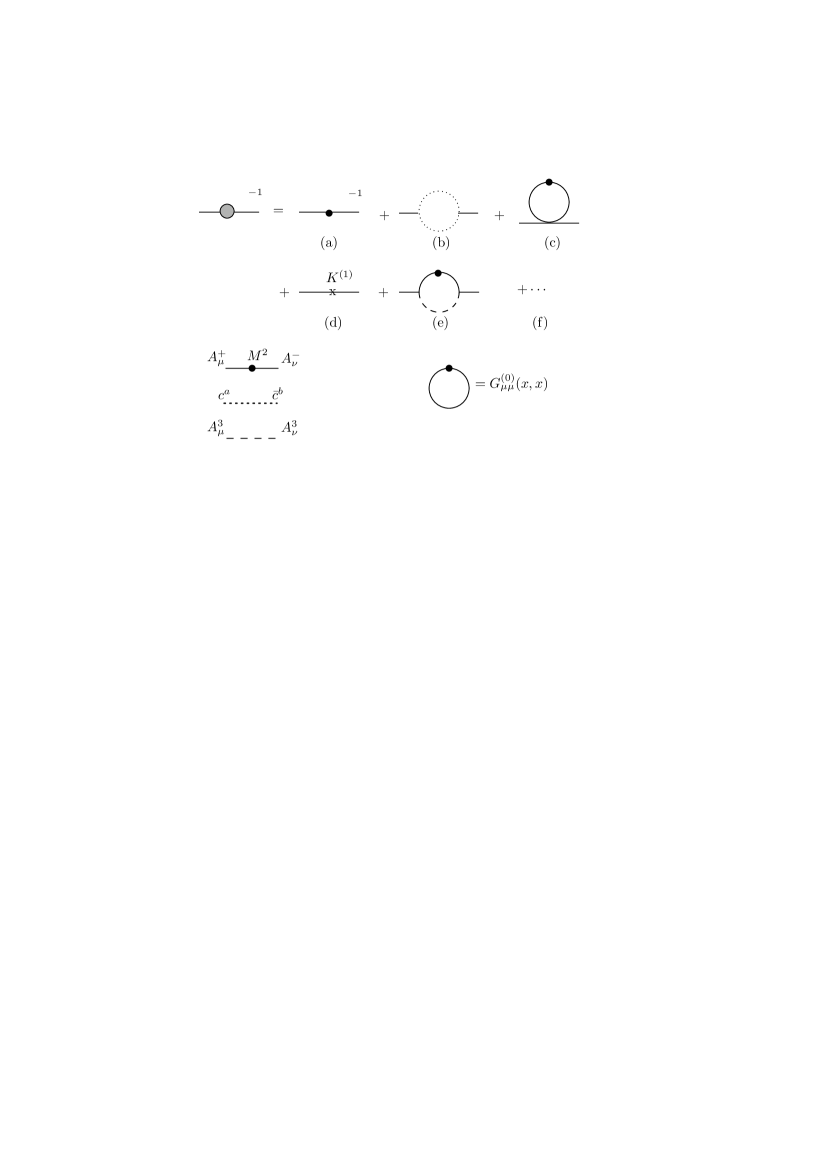
To remove the tachyonic mass terms
| (2.6) |
we introduce the source term
Although the source may depend on the momentum scale, for simplicity, we treat it as constant, and write . To consider the inverse propagator for depicted in Fig. 1 in the limit , we write the free part of the propagator as . Then the diagram in Fig. 1(c) gives the VEV . If subtracts divergent terms of in this limit, the condition
| (2.7) |
removes the tachyonic mass for . Because of the interaction in , this VEV also removes the tachyonic mass for .
2.3 Inclusion of a classical solution
To introduce a classical solution, the gauge field is divided into the classical part and the quantum part , i.e., . As the tachyonic masses come from the ghost loops with the VEV , it is expected that acquires no tachyonic mass. To see it, we divide the gauge transformation as
where . Then, using the gauge-fixing function , the ghost Lagrangian
is obtained. If is replaced by , Eq.(2.2) becomes this Lagrangian. So, the tachyonic mass terms for are
and acquires no tachyonic mass. 111In Ref. hs1 , using the background covariant gauge-fixing, we showed, although the ghost Lagrangian contains , it does not acquire the tachyonic mass.
Next, we consider the effect of the VEV . As in the previous subsection, these tachyonic mass terms for are removed by the VEV in Eq.(2.7). In addition, the interaction in generates the mass term
| (2.8) |
Thus, after integrating out and , an effective low energy Lagrangian becomes
| (2.9) |
where . Namely, although the quantum part is massless, the classical part has the mass . The off-diagonal components have the mass determined by the equation
| (2.10) |
2.4 potential
Now we consider the confining potential. As the classical field , we choose the dual electric potential , that describes the electric monopole solution hs . The color electric current is incorporated by the replacement
where the space-like vector zwa is chosen as with , and . We note this is the Zwanziger’s dual field strength in Ref. zwa . Thus the classical part of in Eq.(2.9) becomes
| (2.11) |
The equation of motion for is
and is solved as
| (2.12) |
If we use Eq.(2.12), Eq.(2.11) becomes
| (2.13) |
3 Cut-off and the mass
In this section, we study Eq.(2.10). The free propagator is calculated in Appendix A as
| (3.1) |
Assuming that exists below a cut-off , we obtain
| (3.2) |
where the -independent term is subtracted.
The VEV depends on the momentum scale . From Eqs.(2.3) and (2.4), we find disappears above the scale . When , behaves as
Namely the maximal value of is , and the left hand side of Eq.(2.10) satisfies
On the other hand, the VEV only depends on the constants and . Since the tachyonic mass should be removed in the overall momentum region completely, using the maximal value of , we interpret Eq.(2.10) as 222If we consider the scale dependent , Eq.(3.2) should be replaced by the integral As is unknown, we cannot calculate it. But it is also -independent.
4 Confining potential
Usually, the potential in Eq.(2.15) is calculated as follows. Let us divide the momentum in into and that satisfies . Then the integral of has the infrared divergence, and the integral of has the ultraviolet divergence. The former divergence is removed by the choice sst ; hs , and the latter divergence is avoided by the cut-off as suz ; mts ; sst ; sst2
| (4.1) |
Eq.(4.1) becomes the linear term in Eq.(1.2). The term has the integral of over the region of , and the Yukawa potential in Eq.(1.2) is obtained.
To introduce a cut-off in a different way, we write the potential as
| (4.2) |
As we stated in Sect. 3, the mass can exist above . From Fig. 1(c), after disappears, it is expected that contributes to the correction for . Since are considered to be massless above , we assume that the cut-off for is , and define Eq.(4.2) as
| (4.3) |
Eq.(4.3) is rewritten as
| (4.4) |
The first term becomes
| (4.5) |
and the second term leads to
| (4.6) |
where () comes from (). Eq.(4.5) gives the usual Coulomb potential
| (4.7) |
Now we consider . To satisfy , the domain of integration is not in Eq.(4.1), but with , i.e.,
Since the integrand is singular at , we choose the anticlockwise path in Fig. 2, and take the limit . Then we obtain
| (4.8) |
If the cut-off is replaced by , becomes the linear term in Eq.(1.2).

Finally, neglecting additive constants, we find becomes
| (4.9) |
Thus the confining potential we propose is
| (4.10) |
In addition to the Coulomb plus linear part, there is the term .
5 Determination of parameters
Although we presented the potential , the values of the parameters and are unknown. To determine them, let us expand a potential as
We assume there is a true confining potential . Then we require the Cornell potential fits well to at a point . This is achieved by choosing and the constant appropriately. 333To determine the three parameters, it is natural to choose appropriate three points . However, in the next step, we must determine so as to the difference between and becomes minimum. Since in contains in the integrand, it is difficult to determine . We impose the conditions
| (5.1) |
and determine and .
Next, we require that the potential fits well to this at , and use the conditions
| (5.2) |
We note, to determine the parameters and , the two conditions with are necessary. However, to determine , the condition with is required.
From Eqs.(1.1) and (4.10), we have
Since Eq.(5.2) with gives , this condition becomes
| (5.3) |
In the same way, the condition leads to
| (5.4) |
and becomes
| (5.5) |
Of course, the true potential is unknown. So, instead of the first step proposed in Eq.(5.1), we choose appropriate values of and . Thus we determine as follows. Choosing the values of the scale parameter and the off-diagonal gluon mass , Eq.(3.4) determines the cut-off . Then, substituting the values of , and into Eqs.(5.3)-(5.5), the quantities , and are determined numerically. As an example, we choose the values
| (5.6) |
We note that the off-diagonal gluon mass GeV in the region of fm was obtained by using SU(2) lattice QCD in the maximal Abelian gauge as . The values and GeV2 come from lattice simulations bali .
Now using the values of and in Eq.(5.6), Eq.(3.4) gives GeV. Next, we substitute this and in Eq.(5.6) into Eqs.(5.3)-(5.5), and solve these equations. The details are explained in Appendix B. The results are
and these values lead to
| (5.7) |
Thus we obtain
| (5.8) |
where
| (5.9) |
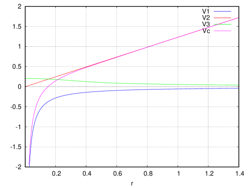
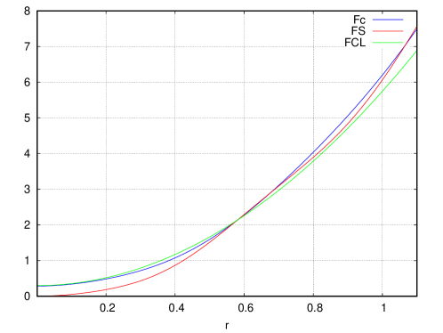
In Fig.3, the potentials and are plotted. Since is a substitute for the Yukawa potential, for is reasonable. Using the values of in Eq.(5.6), becomes
| (5.10) |
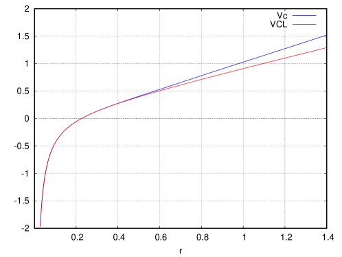
Eqs.(5.8) and (5.10) are plotted in Fig. 4. Since is fitted to at , they fit very well for . However, when becomes large, as and , holds for . In the same way, leads to for .
6 The scales and
In Sect. 5, the scale appears. On the other hand, considering the force , the intermediate scale , which satisfies
| (6.1) |
was proposed so . In successful potential models, this relation holds fairly well. For example, the with cor2 gives . If we substitute in Eq.(5.8) into Eq.(6.1), we obtain
| (6.2) |
where
| (6.3) |
comes from . Eq.(6.2) gives the solution . We note, with in Sect. 5 gives the larger value .
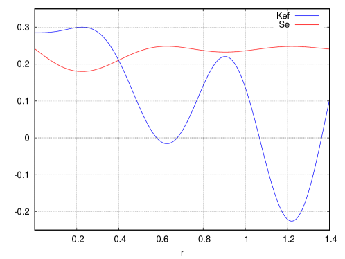
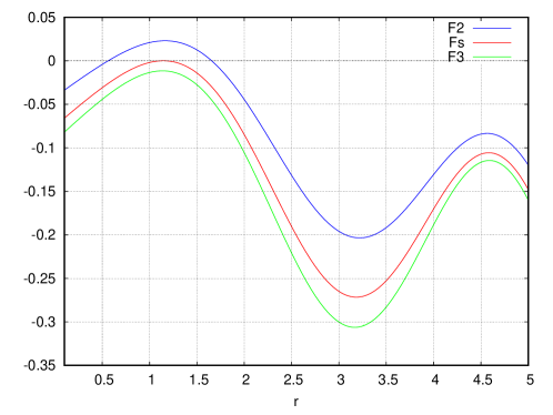
To see the meanings of these scales, the effective Coulomb coupling in Eq.(5.3) and the effective string tension in Eq.(5.4) are plotted in Fig. 5. We find is the maximal value and is the minimal value. Namely is the position where is maximum and is minimum. We also notice that at , and for .
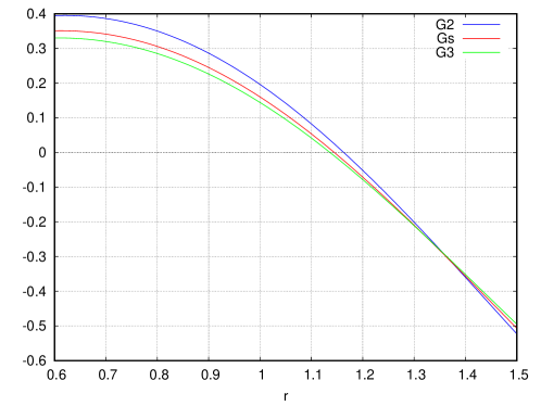
In Fig. 6, and are plotted. We find that satisfies for , and for . Namely, the force-related quantity is almost saturated with the string part above . Especially, as at , we find
Before closing this section, based on the above analysis, we present the potential that fits to better in the region of . When is small, the Coulomb part dominates. So keeping the condition Eq.(5.3) intact, we set . When becomes large, the string part dominates. To determine the value of , it is reasonable to set the condition
| (6.4) |
We find with satisfies Eq.(6.4). We note this satisfies Eq.(6.1) as well.
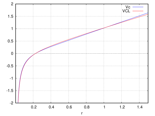
In Fig. 7, the potential and
| (6.5) |
are plotted . As we explained in Sect. 5, the behavior comes about for large . However Eq.(6.5) fits fairly well for .
7 Summary and comments
In this paper, we considered the SU(2) gauge theory, and studied the potential Eq.(2.15). This potential is derived under the gauge field condensation. In Refs. suz ; mts ; sst ; sst2 , the dual Ginzburg-Landau model, which describes the monopole condensation, leads to the potential.
In our approach hs ; hs1 , the ghost condensation appears, and it induces the VEV , that is the lowest term of . If we divide the diagonal gluon as , the classical part acquires the mass , whereas the quantum part is massless. The off-diagonal gluons acquire the mass through Eq.(3.3). The low energy effective Lagrangian is Eq.(2.9). As the classical solution , we choose the electric monopole solution of the dual gauge field hs1 . Then the propagator of leads to the potential Eq.(2.15).
In calculating Eqs.(3.3) and (4.3), ultraviolet cut-off is necessary. Above the scale , although vanishes, the masses and can exist. We assumed that these masses disappear above the cut-off . Then the condition in Eq.(3.4) and the confining potential in Eq.(4.10) are obtained. This potential has the linear potential and, instead of the Yukawa potential, the Coulomb potential and the additional term .
Although we derived , there are unknown parameters. To determine them, we chose the values presented in Eq.(5.6). Then, from Eq.(3.4), the cut-off GeV was obtained. Next, assuming that the Cornell potential with describes a true potential well at some point , we required near . To realize this requirement, the conditions in Eq.(5.2) are imposed. By solving these conditions, , the values of and in Eq.(5.7), and in Eq.(5.8) were obtained.
There are two implicit scales and (or ) in . To understand them, the effective Coulomb coupling in Eq.(5.3) and the effective string tension in Eq.(5.4) were studied. Since contributes to them, they depend on . At , becomes maximum and becomes minimum. For , holds.
If we consider the quantity , we find
Namely the main force between and is the effective Coulomb force for , and the effective string force for .
Although was determined to fit to with at , it becomes larger than for . The Cornell potential is often used to fit lattice simulation data. Can we find that fits to better? To answer this question, we used the above scales. At , Eq.(5.3) was applied to determine . To determine , we used Eq.(6.4) at . Then we obtained with . This potential satisfies Eq.(6.1) at as well, and fits fairly well in the region of .
We make three comments.
(1). In quark confinement, Abelian dominance ei is expected. The lattice simulation in the maximal Abelian gauge shows that the linear part of the potential comes from the Abelian part ss . In the present case, Abelian dominance is realized by the massive classical U(1) field . This field brings about the potential .
Appendix A Propagator for
Referring to Eqs.(2.2) and (2.9), we consider the Lagrangian with the massive gauge fields :
The fields , and mix. The inverse propagators of these fields are
| (A.1) |
and the corresponding propagators are
| (A.2) |
where , and
Under the BRS transformation , as and ,
holds, if the BRS symmetry is not broken spontaneously. When , to make
vanish, we choose . Then Eq.(A.2) becomes
| (A.3) |
Eq.(A.3) shows that mixes with . At the one-loop order, the ghost loop contributes to , and as well. However tachyonic behavior only appears in . In Sect. 3, as the mixing like does not contribute, the propagator
in Eq.(A.3) is used.
Appendix B Solution of Eqs.(5.3)-(5.5)
From Eq.(4.9), we find the derivatives
Then, introducing the variables and , Eqs.(5.3)-(5.5) become
| (B.1) | |||
| (B.2) | |||
| (B.3) |
where is defined in Eq.(6.3), and
By eliminating , Eqs.(B.1) and (B.2) leads to
| (B.4) |
References
- (1) G. Bali, Phys. Rept. 343, 1 (2001).
- (2) E. Eichten et al., Phys. Rev. Lett. 34, 369 (1975).
- (3) E. Eichten et al., Phys. Rev. D 21, 203 (1980).
- (4) G. Ripka, arXiv:hep-ph/0310102.
- (5) T. Suzuki, Prog. Theor. Phys. 80, 929 (1988).
- (6) S. Maedan and T. Suzuki, Prog. Theor. Phys. 81, 229 (1989).
- (7) S. Sasaki, H. Suganuma and H. Toki, Prog. Theor. Phys. 94, 373 (1995).
- (8) H. Suganuma, S. Sasaki and H. Toki, Nucl. Phys. B 435, 207 (1995).
- (9) H. Sawayanagi, Prog. Theor. Exp. Phys. 2019, 033B03 (2019).
- (10) H. Sawayanagi, Prog. Theor. Exp. Phys. 2017, 113B02 (2017).
- (11) R. Sommer, Nucl. Phys. B 411, 839 (1994).
- (12) G. Curci and R. Ferrari, Phys. Lett. B63, 91 (1976).
- (13) H. Sawayanagi, Phys. Rev. D 67, 045002 (2003).
- (14) H. Sawayanagi, Prog. Theor. Phys. 117, 305 (2007).
- (15) D. Zwanziger, Phys. Rev. D 3, 880 (1971).
- (16) K. Amemiya and H. Suganuma, Phys. Rev. D 60, 114509 (1999).
- (17) Z. F. Ezawa and A. Iwazaki, Phys. Rev. D 25, 2681 (1982).
- (18) N. Sakumichi and H. Suganuma, Phys. Rev. D 90, 111501(R) (2014).