Concordance invariant $\Upsilon$ for balanced spatial graphs using grid homology

The $\tau$ invariant and the $\Upsilon$ invariant are defined by Ozsváth, Szabó [4],[6] using knot Floer homology. The $\tau$ invariant and the $\Upsilon$ invariant give homomorphisms from the (smooth) knot concordance group $\mathcal{C}$ to $\mathbb{Z}$ and lower bounds for the slice genus and the unknotting number. The $\tau$ invariant is known to prove the Milnor conjecture $g_{4}(T_{p,q})=\frac{1}{2}(p-1)(q-1)$ [7]. The $\Upsilon$ invariant is a family of concordance invariants $\Upsilon_{t}$ defined for every $t\in[0,2]$ and the slope of the $\Upsilon$ invariant at $t=0$ equals the value of the $\tau$ invariant, so the $\Upsilon$ invariant is stronger than the $\tau$ invariant. The $\Upsilon$ invariant shows that the subgroup of $\mathcal{C}$ generated by topologically slice knots has $\mathbb{Z}^{\infty}$ direct summand [6].

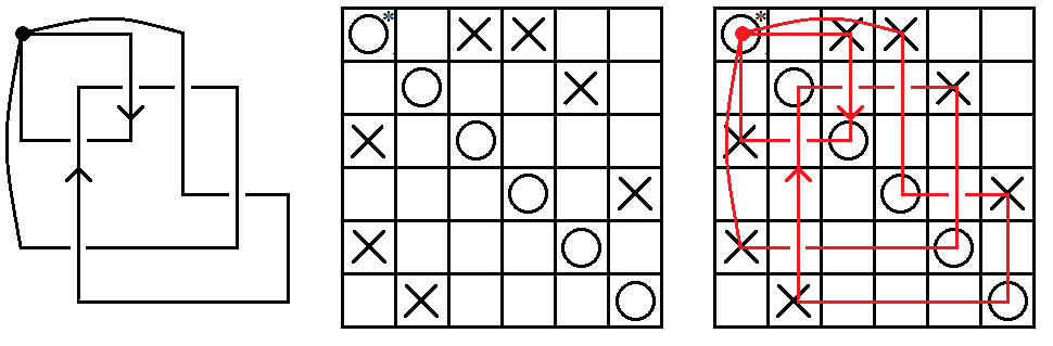
Grid homology is a combinatorial version of knot (link) Floer homology developed by Manolescu, Ozsváth, Szabó, and Thurston [3]. The original definition of knot Floer homology needs gauge theory and pseudo-holomorphic curves. In contrast, grid homology only needs combinatorial procedures such as gazing at a planar figure called a grid diagram (figure 1) and counting some rectangles on the grid diagram.

One of the main research directions of grid homology is to give purely combinatorial proofs for the known properties of knot Floer homology. For example, Sarkar [7] gave a combinatorial reconstruction of the $\tau$ invariant, which we denote $\tau^{grid}$, using grid homology. Sarkar also gave a purely combinatorial proof that the $\tau^{grid}$ is a concordance invariant. As an application of it, a combinatorial proof of the Milnor conjecture was obtained. Földvári [1] defined the $\Upsilon^{grid}$ invariant using grid homology for $t\in[0,2]\cap\mathbb{Q}$ and evaluated the change of values on crossing changes.

A spatial graph is a smooth embedding $f\colon G\to S^{3}$, where $G$ is a one-dimensional CW-complex. We assume that spatial graphs are always oriented. A transverse spatial graph is a spatial graph such that for each vertex $v$, there is a small disk $D\subset S^{3}$ whose center is $v$ separating incoming edges and outgoing edges. In this paper, we need one more condition: a transverse spatial graph is balanced if at each vertex, the number of incoming edges equals the number of outgoing edges.

Harvey, O’Donnol [2] extended grid homology to transverse spatial graphs. Then it is natural to explore generalizing of results of knot Floer Homology to transverse spatial graphs. Vance [8] defined the $\tau^{spatial}$ invariant for balanced spatial graphs as an extension of Sarkar’s $\tau^{grid}$ invariant. As an application of the $\tau^{spatial}$, Vance gave the bounds for the change of the $\tau^{spatial}$ invariant of two links connected by a link cobordism.

In this paper, we first define $\Upsilon^{spatial}$ for balanced spatial graphs for every $t\in[0,2]$ as an extension of Földvári’s knot invariant $\Upsilon^{grid}$. Then we give a combinatorial proof that $\Upsilon^{spatial}$ (and also $\Upsilon^{grid}$) is a concordance invariant of knots. Our $\Upsilon^{spatial}$ contains more information than Földvári’s $\Upsilon^{grid}$ because $\Upsilon^{grid}$ is defined for $[0,2]\cap\mathbb{Q}$ but our $\Upsilon^{spatial}$ is defined for all $[0,2]$.

hhTo construct the $\Upsilon^{spatial}$ invariant, we use the t-modified chain complex $tCF^{-H}(g)$ from the grid chain complex in the same way as the way of Ozsváth, Stipsicz, and Szabó [6] and prove that the homology of the t-modified chain complex $tHF^{-H}(g)$ is (almost) independent of the choice of the graph grid diagram. To define the $\Upsilon$ invariant using knot Floer homology, Ozsváth, Stipsicz, and Szabó used a formal construction of the t-modified chain complex from filtered chain complex $C\mapsto C^{t}$, and to see the invariance, they showed that filtered chain homotopy equivalent complexes $C\simeq D$ are lifted to chain homotopy equivalent complexes $C^{t}\simeq D^{t}$. Applying these ideas and considering the connection between the grid chain complexes and the t-modified chain complexes enable us to define $\Upsilon^{spatial}$ for all $[0,2]$ and to ensure the invariance of the $\Upsilon^{spatial}$.

This section provides an overview of grid homology for transverse spatial graphs. See [2] for details. For grid homology for knots and links, see [3],[5].

A planar graph grid diagram $g$ (figure 1) is a $n\times n$ grid of squares some of which is decorated with an $X$- or $O$- (sometimes $O{}^{*}$-) marking such that it satisfies the following conditions.

1. (i)

   There is just one $O$ or $O{}^{*}$ on each row and column.

2. (ii)

   There is at least one $X$ on each row and column.

3. (iii)

   $O$’s (or $O{}^{*}$’s) and $X$’s do not share the same square.

We denote the set of $O$-markings by $\mathbb{O}$ and the set of $X$-markings by $\mathbb{X}$. We often use the labeling of markings as $\{O_{i}\}_{i=1}^{n}$ and $\{X_{j}\}_{j=1}^{m}$.

For any transverse spatial graph $f$, we can take graph grid diagrams representing $f$. The relation between a spatial graph and representing grid diagram is the following: Drawing horizontal segments from the $O-$ (or $O{}^{*}-$) marking to the $X$-markings in each row and vertical segments from the $X$-markings to the $O-$ (or $O{}^{*}-$) marking in each column and assuming that the vertical segments always cross above the horizontal segments, then we can recover the spatial graph from the corresponding graph grid diagram. We think that $O^{*}$-markings correspond to vertices, $O$- and $X$-markings to the interior of edges of the transverse spatial graph.

A toroidal graph grid diagram is a graph grid diagram that we think it as a diagram on the torus obtained by identifying edges in a natural way. We assume that every toroidal diagram is oriented in a natural way.

Harvey and O’Donnol showed that any two graph grid diagrams representing the same spatial graph are connected by a finite sequence of the graph grid moves. The graph grid moves are the following three moves on the torus (See also [2, Section 3.4])$\colon$

• •

  Cyclic permutation (figure 2) permuting the rows or columns cyclically.

• •

  Commutation^′ (figure 3) permuting two adjacent columns satisfying the following condition; there are vertical line segments $\textrm{LS}_{1},\textrm{LS}_{2}$ on the torus such that (1) $\mathrm{LS}_{1}\cup\mathrm{LS}_{2}$ contain all the $X$’s and $O$’s in the two adjacent columns, (2) the projection of $\mathrm{LS}_{1}\cup\mathrm{LS}_{2}$ to a single vertical circle $\beta_{i}$ is $\beta_{i}$ , and (3) the projection of their endpoints, $\partial(\mathrm{LS}_{1})\cup\partial(\mathrm{LS}_{2})$, to a single $\beta_{i}$ is precisely two points. Permuting two rows is defined in the same way.

• •

  (De-)stabilization^′ (figure 4) let $g$ be an $n\times n$ graph grid diagram and choose an $X$-marking. Then $g^{\prime}$ is called a stabilization^′ of $g$ if it is an $(n+1)\times(n+1)$ graph grid diagram obtained by adding one new row and column next to the $X$-marking of $g$, moving the $X$-marking to next column, and putting new one $O$-marking just above the $X$-marking and one $X$-marking just upper left of the $X$-marking. The inverse of stabilization^′ is called destabilization^′.

We write the horizontal circles and vertical circles which separate the torus into squares as $\bm{\alpha}=\{\alpha_{i}\}_{i=1}^{n}$ and $\bm{\beta}=\{\beta_{j}\}_{j=1}^{n}$ respectively.

A state $\mathbf{x}$ of $g$ is a bijection $\bm{\alpha}\rightarrow\bm{\beta}$. We denote by $\mathbf{S}(g)$ the set of states of $g$. We describe a state as $n$ points on a toroidal graph grid diagram (figure 5).

We think that there are $n\times n$ squares on $g$ that is separated by $\bm{\alpha}\cup\bm{\beta}$. Fix $\mathbf{x,y}\in S$(g), a domain $p$ from $\mathbf{x}$ to $\mathbf{y}$ is a formal sum of the closure of squares satisfying $\partial(\partial_{\alpha}p)=\mathbf{y}-\mathbf{x}$ and $\partial(\partial_{\beta}p)=\mathbf{x}-\mathbf{y}$, where $\partial_{\alpha}p$ is the portion of the boundary of $p$ in the horizontal circles $\alpha_{1}\cup\dots\cup\alpha_{n}$ and $\partial_{\beta}p$ is the portion of the boundary of $p$ in the vertical ones. A domain $p$ is positive if the coefficient of any square is non-negative. Here we always assume that any domain is positive. Let $\pi(\mathbf{x,y})$ denote the set of domains from $\mathbf{x}$ to $\mathbf{y}$.

Consider $\mathbf{x,y\in S}(g)$ that coincide with $n-2$ points. An rectangle $r$ from $\mathbf{x}$ to $\mathbf{y}$ is a domain that satisfies that $\partial r$ is the union of four segments. A rectangle $r$ is an empty rectangle if $\mathbf{x}\cap\mathrm{Int}(r)=\mathbf{y}\cap\mathrm{Int}(r)=\emptyset$. Let $\mathrm{Rect}^{\circ}(\mathbf{x,y})$ be the set of empty rectangles from $\mathbf{x}$ to $\mathbf{y}$.

The grid chain complex $(CF^{-}(g),\partial^{-})$ is a module over $\mathbb{F}[U_{1},\dots,U_{n}]$ freely generated by $\mathbf{S}(g)$, where $\mathbb{F}=\mathbb{Z}/2\mathbb{Z}$ and the $U_{i}$’s are the formal variables corresponding to the $O_{i}$’s in $g$. The differential $\partial^{-}$ is defined as counting empty rectangles by

$$\partial^{-}(\mathbf{x})=\sum_{\mathbf{y}\in\mathbf{S}(g)}\left(\sum_{r\in\mathrm{Rect}^{\circ}(\mathbf{x,y})}U_{1}^{O_{1}(r)}\cdots U_{n}^{O_{n}(r)}\right)\mathbf{y},$$

where $O_{i}(r)=1$ if $r$ contains $O_{i}$ and $O_{i}(r)=0$ otherwise for $i=1,\dots,n$.

There are two gradings for $CF^{-}(g)$, the Maslov grading and the Alexander grading. A planar realization of toroidal diagram $g$ is a planar figure obtained by cutting toroidal diagram $g$ along $\alpha_{i}$ and $\beta_{j}$ for some $i$ and $j$, and putting on $[0,n)\times[0,n)\in\mathbb{R}^{2}$ in a natural way. For two points $(a_{1},a_{2}),(b_{1},b_{2})\subset\mathbb{R}^{2}$, let $(a_{1},a_{2})<(b_{1},b_{2})$ if $a_{1}<b_{1}$ and $a_{2}<b_{2}$. For two sets of finitely points $A,B\subset\mathbb{R}^{2}$, let $\mathcal{I}(A,B)$ be the number of pairs $a\in A,b\in B$ with $a<b$ and let $\mathcal{J}(A,B)=(\mathcal{I}(A,B)+\mathcal{I}(B,A))/2$. Let $m_{i}$ be the number of $X$-markings in the row caontaining $O_{i}$ ($i=1,\dots,n$). Then for $\mathbf{x\in S}(g)$, the Maslov grading $M(\mathbf{x})$ and the Alexander grading $A(\mathbf{x})$ are defined by

(2.1)		$\displaystyle M(\mathbf{x})=\mathcal{J}(\mathbf{x}-\mathbb{O},\mathbf{x}-\mathbb{O})+1,$
(2.2)		$\displaystyle A(\mathbf{x})=\mathcal{J}(\mathbf{x},\mathbb{X}-\sum_{i=1}^{n}m_{i}O_{i}).$

These two gradings are extended to the whole of $CF^{-}(g)$ by

(2.3)

$\displaystyle M(U_{i})=-2,A(U_{i})=-m_{i}\ (i=1,\dots,n).$

Note that the Alexander grading here is the same as Vance’s definition, while the original Alexander grading by Harvey and O’Donnol has values in $H_{1}(S^{3}-f(G))$, where $f\colon G\rightarrow S^{3}$ is the transverse spatial graph represented by $g$. The Alexander grading here is given from the original one by taking the canonical homomorphism $H_{1}(S^{3}-f(G))\rightarrow\mathbb{Z}$ which sends the generators to 1. Also, note that the Alexander grading is not well-defined as a toroidal diagram, however, relative Alexander grading $A^{rel}(\mathbf{x,y})=A(\mathbf{x})-A(\mathbf{y})$ is well-defined.

It is shown that the differential $\partial^{-}$ drops Maslov grading by 1 and preserves or drops Alexander grading, so $(CF^{-}(g),\partial^{-})$ is a Maslov graded, Alexander filtered chain complex [8, Proposition 3.7].

Suppose the $O$-markings are labeled so that $O_{1},\dots,O_{V}$ are $O^{*}$-markings and $O_{V+1},\dots,O_{n}$ are $O$-markings. Let $\mathcal{U}$ be the minimal subcomplex of $CF^{-}(g)$ containing $U_{1}CF^{-}(g)\cup\dots\cup U_{V}CF^{-}(g)$. Then $(\widehat{CF}(g),\widehat{\partial})$ is a Maslov graded, Alexander filtered chain complex over $\mathbb{F}$-vector space obtained by letting $\widehat{CF}(g)=CF^{-}(g)/\mathcal{U}$ and $\widehat{\partial}$ be the map induced by $\partial^{-}$.

We denote by $\{\mathcal{F}^{-}_{m}(g)\}_{m\in\mathbb{Z}}$ (respectively $\{\widehat{\mathcal{F}}_{m}(g)\}_{m\in\mathbb{Z}}$) the Alexander filtration of $CF^{-}(g)$ (respectively $\widehat{CF}(g)$).

Let $CF^{-H}(g)$ be a Maslov graded, symmetrized Alexander filtered chain complex obtained from $CF^{-}(g)$ by using the symmetrized Alexander grading $A^{H}$ rather than the Alexander grading $A$.

The homology of the associated graded object of $CF^{-H}(g)$ is an invariant for balanced spatial graphs [8, Theorem 3.15].

This section provides the definition of the t-modified chain complex $tCF^{-H}(g)$. The t-modified chain complex here is the extension of one of Földvári.

First of all, we define the based ring $\mathcal{R}$ of $tCF^{-H}(g)$.

A set $A\subset\mathbb{R}$ is well-ordered if any subset $A^{\prime}\subset A$ has a minimal element.

The sum in $\mathcal{R}$ is given by the formula

$$\left(\sum_{\alpha\in A}v^{\alpha}\right)+\left(\sum_{\beta\in B}v^{\beta}\right)=\sum_{\gamma\in C=A\cup B\setminus A\cap B}v^{\gamma}\ ,$$

and the product is given by the formula

$$\left(\sum_{\alpha\in A}v^{\alpha}\right)\cdot\left(\sum_{\beta\in B}v^{\beta}\right)=\sum_{\gamma\in A+B}\#\{(\alpha,\beta)\in A\times B|\alpha+\beta=\gamma\}\cdot v^{\gamma},$$

where

$$A+B=\left\{\gamma|\gamma=\alpha+\beta\ for\ some\ \alpha\in A\ and\ \beta\in B\right\}.$$

It is straightforward to check that the above operations are well-defined.

Then we define the t-modified chain complex $tCF^{-H}(g)$. For a domain $p$ as a formal sum of squares, let $O_{i}(p)$ denote the coefficient of the square containing $O_{i}$, and let

$$|\mathbb{O}\cap p|:=\sum_{i=1}^{n}O_{i}(p).$$

We define $|\mathbb{X}\cap p|$ in the same manner.

In this section, we give an alternative definition of the t-modified chain complex using the grid chain complex. See [6, Section 4] for details.

Suppose that $C$ is a finitely generated, Maslov graded, Alexander filtered chain complex over $\mathbb{F}[U]$. Let $\mathbf{x}$ be a generator of $C$ over $\mathbb{F}[U]$, with Maslov grading $M(\mathbf{x})$. Since multiplication by $U$ drops the Maslov grading by 2, elements of Maslov grading $M(\mathbf{x})-1$ are linear combinations of elements of the form $U^{\frac{M(\mathbf{y})-M(\mathbf{x})+1}{2}}\mathbf{y}$, where $\mathbf{y}$ is a generator. Then the differential on $C$ can be written as

(4.1)

$$\partial(\mathbf{x})=\sum_{\mathbf{y}}c_{\mathbf{x},\mathbf{y}}\cdot U^{\frac{M(\mathbf{y})-M(\mathbf{x})+1}{2}}\mathbf{y},$$

where $c_{\mathbf{x},\mathbf{y}}\in\{0,1\}$.

Note that $CF^{-H}_{U}(g)$ is a Maslov graded chain complex but not an Alexander filtered chain complex because the drop in the Alexander grading of each $U_{i}$ differs by (2.3). However, Definition 4.1 works for $CF^{-H}_{U}(g)$ because each generator has its Alexander grading. Therefore we can define the formal t-modified chain complex $(CF^{-H}_{U}(g))^{t}$.

Next, we introduce the following proposition playing an important role in this paper.

Again note that this proposition can be applied as $CF^{-H}_{U}(g)\mapsto(CF^{-H}_{U}(g))^{t}$ even if $CF^{-H}_{U}(g)$ is just Maslov graded chain complex with $A^{H}$ grading only for generators. Similar to (4.1), Maslov graded chain map $f\colon CF^{-H}_{U}(g)\rightarrow CF^{-H}_{U}(g^{\prime})$ can be written as

$$f(\mathbf{x})=\sum_{\mathbf{y}}c_{\mathbf{x},\mathbf{y}}\cdot U^{\frac{M(\mathbf{y})-M(\mathbf{x})}{2}}\mathbf{y},$$

then the corresponding graded chain map is

$$f^{t}(\mathbf{x})=\sum_{\mathbf{y}}c_{\mathbf{x},\mathbf{y}}\cdot v^{\mathrm{gr}_{t}(\mathbf{y})-\mathrm{gr}_{t}(\mathbf{x})}\mathbf{y}.$$

This construction gives induced chain homotopy equivalence for the t-modified chain complexes.

This section provides the filtered chain homotopy equivalences for grid chain complexes connected by each graph grid move. These filtered chain homotopy equivalences are lifted into chain homotopy equivalences for the t-modified chain complexes by applying Proposition 4.4. Chain homotopy equivalences for a cyclic permutation and a commutation^′ are already known. We mainly observe the case of stabilization^′.

References

- [1] Viktória Földvári, The knot invariant using grid homologies, J. Knot Theory Ramifications 30 (2021), no. 7, Paper No. 2150051, 26. MR 4321933
- [2] Shelly Harvey and Danielle O’Donnol, Heegaard Floer homology of spatial graphs, Algebr. Geom. Topol. 17 (2017), no. 3, 1445–1525. MR 3677933
- [3] Ciprian Manolescu, Peter Ozsváth, Zoltán Szabó, and Dylan Thurston, On combinatorial link Floer homology, Geom. Topol. 11 (2007), 2339–2412. MR 2372850
- [4] Peter Ozsváth and Zoltán Szabó, Knot Floer homology and the four-ball genus, Geom. Topol. 7 (2003), 615–639. MR 2026543
- [5] Peter S. Ozsváth, András I. Stipsicz, and Zoltán Szabó, Grid homology for knots and links, Mathematical Surveys and Monographs, vol. 208, American Mathematical Society, Providence, RI, 2015. MR 3381987
- [6] by same author, Concordance homomorphisms from knot Floer homology, Adv. Math. 315 (2017), 366–426. MR 3667589
- [7] Sucharit Sarkar, Grid diagrams and the Ozsváth-Szabó tau-invariant, Math. Res. Lett. 18 (2011), no. 6, 1239–1257. MR 2915478
- [8] Katherine Vance, Tau invariants for balanced spatial graphs, J. Knot Theory Ramifications 29 (2020), no. 9, 2050066, 29. MR 4152956