Concatenating Binomial Codes with the Planar Code

As discussed above the only logical gate we need to enact on RSB encoded qubits in our computational scheme is the controlled phase $C_{Z}$ gate. The $C_{Z}$ gate may be realised by a controlled rotation at the physical level generated by a cross-Kerr interaction between the modes [21, 31]

	$\displaystyle H_{\textsc{CROT}_{ij}}$	$\displaystyle=-\Omega\hat{n}_{i}\otimes\hat{n}_{j}$
	$\displaystyle\textsc{CROT}_{ij}$	$\displaystyle=e^{-iH_{\textsc{CROT}_{ij}}t_{\rm gate}}$
		$\displaystyle=e^{\frac{i\pi\hat{n}_{i}\otimes\hat{n}_{j}}{NM}}$		(6)

where modes $i,j$ involve RSB qubits with discrete rotational symmetry of order $N,M$ respectively. Loss is the dominant imperfection in our model and if the cross-Kerr gate is slow the effect of loss is exacerbated. Both the strength of the loss and the time required for the gate are captured by the parameter $\gamma=\kappa t_{gate}$ which we will use to characterize the noise level. The gate time is chosen such that $\Omega t_{\rm gate}=\pi/NM$ thus $\gamma$ is proportional to the photon loss rate and inversely proportional to the cross-Kerr nonlinearity. In all that follows we only consider CROT gates between identical encodings, so $N=M.$

Note that low cross-Kerr nonlinearity in practical devices might lead to a different coupling non-linearity being preferred, such as a SNAIL [32]. In this case as well the effect of loss will depend on the per photon loss probability during a gate. So while the details of code performance would differ, we expect qualitatively similar results for such a gate.

The other RSB operation we need is a destructive single qubit X measurement, which we investigate in Sec.III.1.

To describe the noise due to photon loss, we use the framework of quantum trajectory theory [33] to analyse a master equation describing losses occurring on each qubit during the implementation of the CROT gate. The master equation describing the combined effects of the gate and loss is

$\displaystyle\dot{\rho}=-i[H_{\textsc{CROT}_{12}},\rho]+\kappa\sum_{i=1}^{2}\mathcal{D}[\hat{a_{i}}]\rho$

(7)

where $\hat{a}_{1}=\hat{a}\otimes\mathbb{I},\hat{a}_{2}=\mathbb{I}\otimes\hat{a}$, $\mathcal{D}[L]\rho=L\rho L^{\dagger}-L^{\dagger}L\rho/2-\rho L^{\dagger}L/2$ is the Lindblad superoperator. We will describe the effects of loss using the parameter $\gamma=\kappa t_{\rm gate}$,

In the trajectory approach the density matrix can be written as a sum over the number of photon emission events that occur during the gate. Each term involves an integral over the emission time of the photons. As described in more detail in Appendix A we commute the loss past the CROT gate in each such term so that we are left with an effective error operator acting on each qubit.

We will introduce a notation that can be generalized to the case of $M$ modes. Suppose that the times for which losses occur on mode 1 are listed in a vector $\mathbf{t}_{1}$. We will suppose that these emission times are arranged in time order such that for times $t_{m},t_{m+1}\in\mathbf{t}_{1}$ we have $t_{m+1}>t_{m}$. Similarly emission times for mode 2 are $\mathbf{t}_{2}$. We will sometimes need to refer to the emission times for all modes, and we do this by defining an array of emission time vectors $\mathbf{t}=\{\mathbf{t}_{1},\mathbf{t}_{2}\}.$ The number of photon emissions for mode $a$ is $j_{a}=|\mathbf{t}_{a}|$ the number of entries in the vector $\mathbf{t}_{a}$. The total number of photon emissions $k$ is the sum of the $j_{a}$, so for two modes we have $j_{1}+j_{2}=k$. Then the noisy CROT gate with a fixed number of photon emissions can be expressed as

$\displaystyle\widetilde{\textsc{CROT}}_{12,\mathbf{t}}$

$\displaystyle=\hat{E}_{1,{\mathbf{t}}}\hat{E}_{2,{\mathbf{t}}}\textsc{CROT}_{12}$

(8)

where $\hat{E}_{{\mathbf{t}}},\hat{E}_{{\mathbf{t}}}$ are error operators acting on qubits 1,2 respectively, given by

	$\displaystyle\hat{E}_{1,{\mathbf{t}}}=$	$\displaystyle\sqrt{\kappa}^{j_{1}}e^{\kappa\tau(\mathbf{t}_{1})/2}e^{i\Omega\tau(\mathbf{t}_{2})\hat{n}_{1}}\hat{a}_{1}^{j_{1}}e^{-\kappa t_{\rm gate}\hat{n}_{1}/2}$		(9a)
	$\displaystyle\hat{E}_{2,{\mathbf{t}}}=$	$\displaystyle\sqrt{\kappa}^{j_{2}}e^{\kappa\tau(\mathbf{t}_{2})/2}e^{i\Omega\tau(\mathbf{t}_{1})\hat{n}_{2}}\hat{a}_{2}^{j_{2}}e^{-\kappa t_{\rm gate}\hat{n}_{2}/2}.$		(9b)

This expression is derived in the Appendix A, specifically Eq. A.1. The effective delay parameters $\tau(\mathbf{t}_{a})$ appearing in these expressions are given by

$$\tau(\mathbf{t}_{a})=j_{a}t_{\rm gate}-\sum_{t_{m}\in\mathbf{t}_{a}}t_{m}.$$

(10)

The various factors in $\hat{E}_{1,\mathbf{t}}$ have a natural interpretation. $\hat{E}_{1,{\mathbf{t}}}$ removes $j_{1}$ photons from mode $1$, hence the factor $\hat{a}_{1}^{j_{1}}$. The probability of an event with this number of photon emissions, and the resulting conditioning of the wavefunction, are described by the constant factor $\sqrt{\kappa}^{j_{1}}\exp(\kappa\tau(\mathbf{t}_{1})/2)$ and the non-unitary operator $\exp(-\kappa t_{\rm gate}\hat{n}_{1}/2)$. Finally the action of the gate during the photon loss means that photon loss events on the neighbouring mode $2$ lead to a phase shift on mode 1. This correlated noise process is described by the unitary factor $\exp[i\Omega\tau(\mathbf{t}_{2})\hat{n}_{1}]$. It has very significant consequences for the performance of error correction as we will see.

Turning now to the multimode case where we will need to perform many simultaneous CROT gates. Specifically the gates to be performed are represented by a graph $G=(V,E)$ where the vertices $V$ represent qubits and the edges $E$ represent the location of the gates. We will also use the notation of neighbourhoods - that is, a qubit $i$ is said to be in the neighbourhood of qubit $j$, $i\in\mathcal{N}(j)$, if qubits $i,j$ share an edge. We consider applying all CROT gates simultaneously. Using the same notations as for the two-qubit case, we can express the net noise operator for a qubit $a$ as

$\displaystyle\hat{E}_{a,\mathbf{t}}=\sqrt{\kappa}^{j_{a}}e^{\kappa\tau(\mathbf{t}_{a})/2}\left(\prod_{b\in\mathcal{N}(a)}e^{i\Omega\tau(\mathbf{t}_{b})\hat{n}_{a}}\right)\hat{a}_{a}^{j_{a}}e^{-\kappa t_{\rm gate}\hat{n}_{a}/2}.$

(11)

Note that the mode $a$ acquires a phase shift for a photon emission on any neighbouring qubit.

The overall effect of the noise for a given set of photon emission times $\mathbf{t}$ is given by the operator

$$\tilde{U}_{\mathbf{t}}=\left(\prod_{a=1}^{M}\hat{E}_{a,\mathbf{t}}\right)\prod_{e\in E}\textsc{CROT}_{e_{1},e_{2}}$$

(12)

This equation, derived in the Appendix as equation A.1, expresses the noise as an ideal gate followed by a modified photon loss noise operator. We can think of the overall effect of this noise as defining a noise operator that acts on the ideal cluster state as follows

$\displaystyle\tilde{\Gamma}_{\mathbf{t}}(\rho_{CS})$

$\displaystyle=\tilde{U}_{\mathbf{t}}\left(|+\rangle\langle+|\right)^{\otimes M}\tilde{U}^{\dagger}_{\mathbf{t}}$

(13)

where

$\displaystyle\rho_{CS}=U\left(|+\rangle\langle+|\right)^{\otimes M}U^{\dagger}$

(14)

and $U$ is the ideal gate with $\kappa=0$ and no photon loss events.

This leaves us to determine how to correctly sample a set of emission times $\mathbf{t}$. We show in Appendix A that the probability distribution for photon emission times is unnaffected by the application of the CROT gates. This greatly simplifies our simulations since the photon emission times can be determined independently for each qubit according to a probability distribution that is independent of the particular choice of $G$. The details of the sampling of emissions times $\mathbf{t}$ are givein in Appendix A.2.

A cluster state can be associated to a graph $G=(V,E)$ where vertices represent qubits. Two vertices share an edge if the two qubits of the cluster state are entangled via a ${C}_{Z}$ gate. In our model, each vertex of the graph represents an RSB qubit, and vertices share an edge if the qubit pair is entangled via a CROT gate. The cluster state provides the resource for the quantum computation. Computation will be carried out by single qubit measurements, which will be elaborated upon in Sec. II.3.

We begin by constructing a 1D cluster state and using it to teleport a qubit along the line. For a length $M$ 1D cluster state, we prepare a single qubit in an arbitrary state $|\psi\rangle,$ and the remaining qubits in the $|+\rangle$ state. We then entangle qubits in a line by applying $C_{Z}$ between adjacent qubits. We then measure each qubit in the X basis, which teleports the logical state from the first qubit, down the chain to the final qubit.

We can understand the 1D cluster state in terms of its stabilisers, as in [36] for example. Initially, the logical operators describing the 1D chain will simply be $X_{L}=X_{1},Z_{L}=Z_{1}$ and before the $C_{Z}$ gates the stabiliser group is given by $S=\{X_{1},X_{2},...,X_{n}\}.$ After applying ${C}_{Z}$ gates, operators transform as

	$\displaystyle Z_{i}$	$\displaystyle\rightarrow Z_{i}$
	$\displaystyle X_{i}$	$\displaystyle\rightarrow X_{i}\prod_{j\in\mathcal{N}_{i}}Z_{j}$		(15)

where $\mathcal{N}_{i}$ denotes all qubits which are entangled to qubit $i$ by a ${C}_{Z}$ gate. This causes logicals and stabilisers to transform as

	$\displaystyle Z_{L}$	$\displaystyle=Z_{1}$
	$\displaystyle X_{L}$	$\displaystyle=X_{1}Z_{2}$
	$\displaystyle S$	$\displaystyle=\{X_{1}Z_{2},Z_{1}X_{2}Z_{3},...,Z_{M-1}X_{M}\}.$		(16)

At the conclusion of the $X$ measurements the first $M-1$ qubits are left in $X$ eigenstates and by multiplication with stabilizers we find that the logicals become $Z_{L}=Z_{M}$ and $X_{L}=X_{M}$ reflecting teleportation along the chain.

It is useful to consider how loss at any given location on the chain affects the performance of the scheme. Loss on qubit $i$ propagates through the controlled rotation (${C}_{Z}$) to act as dephasing on qubits $i\pm 1$. In our simulations of this teleportation scheme we assess performance by assuming that the final qubit in the chain has no noise and applying a noise-free recovery to assign a fidelity to the teleportation procedure.

In order to construct the 2D surface code in Fig. 2, we start with parallel 1D cluster states, prepared as before and entangle every odd (primal) qubit of each 1D cluster with the corresponding primal qubit of its neighbouring 1D cluster state, via a dual qubit prepared in the $|+\rangle$ state. Every second qubit of the 1D cluster state is also a dual qubit. The resulting cluster state is depicted in Fig. 4. Measuring every qubit in the X basis realises a measurement of parity checks of primal stabilisers given by a product of $X$ on qubits around a primal plaquette. A primal plaquette stabiliser checks for $Z$ type errors on that plaquette. More explicitly, consider the stabilisers of the cluster state. For a plaquette $p$ of the cluster state, the associated stabiliser is $S_{p}=\prod_{e\in p}X_{e}$, where $e$ denote the primal qubits represented by the edges of the given plaquette as in Fig. 3. To teleport logical information across the 2D foliated state, we measure both primal and dual qubits in the X basis. This also provides stabiliser outcomes, from which we extract the error syndrome.

Having obtained the error syndrome, error correction can be carried out in the usual way [16, 17]. We use a minimum weight perfect matching (MWPM) algorithm to match up pairs of violated stabilisers in the error syndrome in a way that minimises the total distance between pairs of violated stabilisers. The paths between violated stabilisers given by MWPM determine which qubits have experienced errors and therefore give the Pauli correction to which the final logical state with be subject. After the correction has been applied, the simulation can perform a hypothetical logical measurement that determines if the correction has succeeded, or if it has failed and the code has suffered a logical error.

The model we simulate can either be viewed as the foliated 1D repetition code, or equivalently a single 2D timeslice of plaquette stabilizers of the surface code. The noise model we adopt for this scheme includes photon loss occurring during gates and measurement errors on single qubit X measurements, the latter of which arise naturally from the realistic measurement model employed. In the commonly used phenomenological error models for the surface code, both these noise sources map to gate noise rather than phenomenological measurement noise, so that we are still able to observe an error correction threshold for this scheme. Note however that there is only a single logical operator that can be corrected. Therefore while it is possible to learn a lot about the interplay between loss and measurement errors in this code concatenation scheme, a larger scale simulation corresponding to a $2+1D$ surface code simulation would still be desirable.

The ideal realisation of a phase measurement of a bosonic mode is simply the projector onto an (unnormalised) phase eigenstate [37]. This measurement model is very hard to implement, however we include it in simulations as a benchmark of the best possible measurement to which we can compare the other schemes implemented. It has POVM elements

$\displaystyle\hat{F}_{\mathrm{c}}(\phi)$

$\displaystyle=\frac{1}{2\pi}|\phi\rangle\langle\phi|$

(18)

where the phase eigenstate is $|\phi\rangle=\sum_{n=0}^{\infty}e^{i\hat{n}\phi}|n\rangle.$

Heterodyne measurement involves simultaneous homodyne measurements of orthogonal quadratures of a bosonic mode, resulting in adding noise to both quadratures. Heterodyne measurement projects the qubit onto the coherent state $|\alpha\rangle\langle\alpha|$. We can obtain then obtain the phase as $\mathrm{arg}(\alpha)=\phi.$ The POVM for heterodyne measurement with outcome $\alpha$ is

$\displaystyle\hat{F}_{\mathrm{coh}}(\alpha)$

$\displaystyle=\frac{1}{\pi}|\alpha\rangle\langle\alpha|.$

(19)

and

$$\hat{F}_{\mathrm{h}}(\phi)=\int_{0}^{\infty}\hat{F}_{\mathrm{coh}}(re^{i\phi})dr.$$

(20)

Adaptive Homodyne Measurement (AHD) [29] is a better performing alternative to heterodyne measurement. Ordinary homodyne measurement involves the measurement of a single quadrature of the harmonic oscillator mode. It has lower noise than heterodyne measurement but cannot determine the phase of the bosonic mode. In AHD measurement, however, the phase $\theta$ of the local oscillator field is continuously updated based on prior measurements. This rotates the quadrature that is being measured and the scheme is designed to lock in of the phase of the field. Various adaptive schemes are possible we use the Mark II scheme from [29]. The AHD POVM elements are determined by a specific choice of the matrix $H_{mn}$ that appears in Eq. 17, which is defined in Appendix B.

A detailed discussion of both AHD and canonical phase measurement schemes can be found in [29]. An experimental realisation of AHD measurement is described in [38].

In our scheme phase measurements are used to implement $X$ basis measurements of a RSB code. The phase measurement must be able to resolve angles less than $\pi/N$ in order to distinguish qubit states. Thus for a fixed phase measurement it becomes harder to perform qubit measurement as $N$ increases. Neither AHD nor heterodyne measurements provide ideal projective qubit measurements. Both have inherent measurement error which is dependent upon the mean photon number, in addition to the requirement to resolve angles of order $\pi/N$.

Since in this setting we just require the ability to distinguish the two qubit $X$-eigenstates based on phase measurement, we will use a Qubit State Inference (QSI) procedure to achieve this. If the inferred value of the qubit state differs from ‘actual’ state of the qubit determined by our simulation then that constitutes a qubit measurement error. As we will explain in greater detail below this QSI procedure can be chosen to partial compensate from the phase errors that we have seen occur correlated to photon losses on neighbouring qubits.

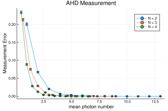
In Figs. 5,6 the data for the measurement error rate as a function of mean photon number is generated numerically. We assume $\gamma=0$ in order to decouple the measurement error from the noise due to photon loss. We then simulate many shots of qubit measurement and calculate the fraction of shots where the logical state as given by the Qubit State Inference, see Sec. III.2, differs from the actual answer found according to Eq. 39. By varying $K$, for fixed $N,$ we vary the mean photon number.

Fig. 5 shows the measurement error $q$ as a function of $\bar{n}$ for heterodyne measurement, for binomial codes of different $N.$ We see that for a given $q$, codes of higher $N$ will have a higher mean photon number.

Fig. 6 shows measurement error as a function of mean photon number for AHD measurement. Not only is the overall measurement error much lower than in the heterodyne case, as expected, but also the measurement error is more consistent across $N$ values. As we will see in Sec. III.6, this has a significant impact on threshold values.

It is important to note that the ‘measurement error’ we are referring to is measurement error at the level of the bosonic mode. This manifests as Pauli errors of the binomial code qubits, rather than as errors in the binomial code single qubit $X$ measurement outcomes. Correcting binomial code qubit measurement outcomes would require multiple measurement rounds. Measurement error in our context contributes to Pauli noise independently from noise due to photon loss.

The binning algorithm utilises the discrete rotational symmetry of RSB codes to straightforwardly bin the phase measurement in the complex plane according to the position of the logical plus and minus states in phase space. Fig. 7 below represents a binning algorithm QSI for an $N=2$ RSB code.

For a three qubit 1D cluster state, the maximum likelihood QSI uses the phase measurement outcomes of the first two qubits to simultaneously infer the states of these qubits. It takes the full noise channel into account for each qubit, and therefore is the most accurate of the QSI techniques we examine. The maximum likelihood QSI works by calculating the probability of the two qubits being in states $i,j$ given their phase measurement outcomes $\phi_{1},\phi_{2}$ and choosing $i,j$ which maximise this probability.

To design our QSI techniques we analyse their performance relative to a simplified noise model where the photon loss occurs before the CROT gates. The loss may be commuted past the CROT gates and will spread to dephasing noise on adjacent qubits. This is in contrast to how we model the noise to which the bosonic modes are subject in our full simulations where loss occurs $during$ the CROT gates, as described in Sec. 14. We use a simpler noise model to design our QSI techniques in order to make them tractable to implement and analyse numerically. Consequently, for the QSI techniques we model photon loss using Kraus operators for photon loss of order $k$

$\displaystyle\hat{A}_{k}=\frac{1}{\sqrt{k!}}(1-e^{-\gamma})^{k/2}e^{\frac{-\gamma\hat{n}}{2}}\hat{a}^{k}.$

(21)

Here the parameter $\gamma$ describes the loss probability for each photon. It corresponds to $\kappa t_{\rm gate}$ in the full model discussed previously in which photon losses can occur an any time. The dephasing operators acting on qubit $i$, given by the commutator with the $\textsc{CROT}_{ij}$ of loss on qubit $j$, are

$\displaystyle\hat{C}_{k}=e^{\frac{-i\pi k\hat{n}_{i}}{N^{2}}}.$

(22)

Suppose that the first two qubits in the cluster have measurement outcomes $\phi_{1},\phi_{2}$ and we aim to infer qubit states $i_{1},i_{2}\in\{\pm 1\}$ in order to obtain the Pauli correction we need to apply to qubit three. We will define the likelihood function $\mathcal{L}(i_{1},i_{2}|\phi_{1},\phi_{2})$ which is given by the conditional probability $p(\phi_{1},\phi_{2}|i_{1},i_{2})$ for the phase measurement outcomes given the initial qubit states.

Each qubit of the cluster is subject to noise due to photon loss as well as dephasing from the photon loss ocurring on neighbouring qubits. Therefore

$\displaystyle\mathcal{L}(i_{1},i_{2}|\phi_{1},\phi_{2})=\sum_{k,k^{\prime}=0}^{\infty}{\rm Tr}\left[\left(F(\phi_{1})\otimes\hat{F}(\phi_{2})\right)\left(\hat{C}_{k^{\prime}}\hat{A}_{k}|i_{1}\rangle\langle i_{1}|\hat{A}^{\dagger}_{k}\hat{C}^{\dagger}_{k^{\prime}}\otimes\hat{C}_{k}\hat{A}_{k^{\prime}}|i_{2}\rangle\langle i_{2}|\hat{A}_{k^{\prime}}^{\dagger}\hat{C}^{\dagger}_{k}\right)\right].$

(23)

Explicitly, maximum likelihood QSI chooses $i,j$ giving

$\displaystyle\mathrm{argmax}_{i,j}\mathcal{L}(i,j|\phi_{1},\phi_{2}).$

(24)

For schemes with more qubits the exact maximum likelihood QSI can be formulated in the same way. However it becomes intractable as the number of qubits in the cluster state is increased. For this reason we consider an approximation that can be performed efficiently.

We define a local maximum likelihood QSI that uses a local approximation of the noise channel acting on any given qubit to obtain an efficient approximation for the likelihood function.

The form of the $\mathcal{L}(i_{a}|\phi)$, likelihood function for the qubit $a$ being in state $i$ conditioned upon its phase measurement outcome $\phi$, depends upon the number of qubits to which the qubit in question is entangled. Suppose that the qubits entangled to a specific qubit $a$ are denoted by $l\in\mathcal{N}(a).$ Let the state of qubit $l$ be $i_{l}$ and the state of all the qubits will be indicated by $\vec{i}$. Let $\mathcal{S}$ denote the set containing all vectors $\vec{j}$ of length $|\mathcal{N}(a)|$ with entries $0\leq j_{l}\leq u$ indicating the number of photon emissions on the mode $l$. Let

$\displaystyle{\rho_{i_{a}}}$

$\displaystyle=\sum_{k=0}^{u}\hat{A}_{k}|i_{a}\rangle\langle i_{a}|\hat{A}_{k}^{\dagger}$

(25)

and

$\displaystyle\mathcal{O}_{a,\vec{i}}$

$\displaystyle=\sum_{\vec{j}\in\mathcal{S}}p_{\vec{i}}(\vec{j})\hat{C}_{\vec{j}}\rho_{i_{a}}\hat{C}^{\dagger}_{\vec{j}}$

(26)

Where the a priori photon emission probabilities are

	$\displaystyle p_{\vec{i}}(\vec{j})$	$\displaystyle=\prod_{l\in\mathcal{N}(a)}p_{i_{l}}(j_{l})$
		$\displaystyle=\prod_{l\in\mathcal{N}(a)}\mathrm{Tr}(\hat{A}_{j_{l}}|i_{l}\rangle\langle i_{l}|\hat{A}_{j_{l}}^{\dagger})$		(27)

and

$$\hat{C}_{\vec{j}}=\prod_{l\in\mathcal{N}(a)}\hat{C}_{j_{l}}$$

(28)

Then we define the approximate likelihood function to be

$\displaystyle\mathcal{L}_{LL}(\vec{i}|\phi)$

$\displaystyle=\prod_{a=1}^{M}\mathrm{Tr}\left[\hat{F}(\phi)\mathcal{O}_{a,\vec{i}}\right]$

(29)

where we truncate the two sums over numbers of photon losses at $u$ for numerical tractability. Given $p(i|\phi)$ the local maximum likelihood QSI works by choosing $i$ as follows

$\displaystyle\mathrm{argmax}_{\vec{i}}\mathcal{L}_{LL}(\vec{i}|\phi).$

(30)

We performed simulations of the minimal instance of the binomial encoded 1D cluster state scheme with a 3-qubit cluster state. Fig. 8 below quantifies the performance of the different measurement schemes. We see that both canonical phase and AHD measurement schemes significantly outperform heterodyne. Furthermore, there does not appear to be a notable difference between the performance of AHD and canonical phase measurements. This indicates that AHD is a good alternative to the optimal canonical phase measurement. Note that the nonzero infidelity at zero $\gamma$ is due to the measurement error inherent described in Sec. III.1.4. Even in the absence of photon loss, due to the finite mean photon number of the binomial encoded qubits, measurement error will lead to qubit-level errors.

We now examine a numerical comparison of the performance of the binning algorithm QSI, maximum likelihood QSI and local maximum likelihood QSI for the three qubit cluster state telecorrection scheme. These qubit state inference techniques are described in detail in Sec. III.2.

Fig. 9 shows the performance of the three QSI techniques for a 3-qubit cluster state with binomial code qubits, as a function of the loss parameter $\gamma.$ As expected, for no loss the QSI technqiues converge on the same value of infidelity. However as $\gamma$ is increased, the binning algorithm performs significantly worse than both the maximum likelihood and local maximum likelihood QSI techniques. Notably, the performance of maximum likelihood and local maximum likelihood is statistically identitical here, indicating that the local maximum likelihood QSI is a good replacement for the full maximum likelihood QSI.

Together these results indicate that adaptive phase measurement combined with a local maximum likelihood QSI is a considerable improvement on the straightfoward heterodyne and binning approach to qubit measurement for the binomial code.

For the purpose of numerical tractability when simulating these larger systems, we introduce an X-basis Pauli twirl for the RSB qubits. We show in Appendix C that in the limit where $\gamma=0$ the twirl has no effect on the measurement statistics and this approximation becomes exact. For non-zero photon loss the twirled noise model is only approximately the same as the physical photon loss model. By removing certain coherences in the photon loss error model the twirl enables simulations to find the threshold of the planar code. We do not expect that the twirl qualitatively changes our results. Simulations that avoid it would require much more expensive simulations, for example based on tensor network simulations [40].

We define the twirl as a mapping $\mathcal{P}_{X_{i}}$ to each qubit $i$ of the RSB code cluster state. The X-basis Pauli twirl acting on a state $\rho$ is given by

$\displaystyle\mathcal{P}_{X_{a}}(\rho)$

$\displaystyle=|+\rangle\langle+|_{a}\otimes\langle+|\rho|+\rangle_{a}+|-\rangle\langle-|_{a}\otimes\langle-|\rho|-\rangle_{a}.$

(33)

Note that while the twirl defined here affects qubit $a$, the density matrix $\rho$ describes the state of the whole set of qubits, not all of which are affected by the twirl. The operator $\langle-|\rho|-\rangle_{a}$ acts on the qubits that are not affected by the twirl.

Consider the first $X$ measurement to be performed on qubit $a$ given times and locations of the photon emissions labelled by $\mathbf{t}$. The state of the remaining qubits for a given phase measurement outcome $\phi_{a}$ will be

$$\rho_{\phi_{a},\mathbf{t}}=\mathrm{Tr}_{a}[\hat{F}_{a}(\phi_{a})\tilde{\Gamma}_{\mathbf{t}}(\rho)]$$

(34)

The norm of this state relates to the probability of the measurement outcome, and in fact we will only be interested in integrals over values of $\phi_{a}$ that map to a given outcome $\pm$ for qubit $a$.

In our simulations we replace these states with states where a $X$-basis twirl is applied prior to the measurement:

$$\bar{\rho}_{\phi_{a},\mathbf{t}}=\mathrm{Tr}_{a}\{\hat{F}_{a}(\phi_{a})\tilde{\Gamma}_{\mathbf{t}}[\mathcal{P}_{X_{a}}(\rho)]\}$$

(35)

To see why this replacement could be justified, let $M_{\pm}$ denote the POVM elements of the noise-plus-measurement-plus-QSI process that is applied to the ideal RSB code qubits and aggregates the phase measurements into the $\pm 1$ outcomes for the measurement. The application of the Pauli twirl $\mathcal{P}_{X}$ to this encoded ideal initial state is justified so long as $M_{\pm}$ is diagonal in the X-basis of the RSB code qubit since in this case $\mathcal{P}^{\dagger}_{X}[M_{\pm}]=M_{\pm}$. For the case that $\gamma=0$ we provide a proof that $\mathcal{P}^{\dagger}_{X}[M_{\pm}]=M_{\pm}$ in the case of the binning QSI in Appendix C.

Note that this replacement works only in the case where, as here, we are interested in some averaged quantity for the schemes such as average entanglement fidelity for a logical qubit channel. If we inspected the data conditioned on phase measurements analysed in some more fine grained way then this twirling approximation is not necessarily justified.

This twirl dramatically simplifies our numerical implementation. Suppose that the ideal initial cluster state of the scheme is $\rho$. So in particular $\rho$ is in the codespace of the RSB code. Consider measuring qubit $a$ of the cluster as before. Then measuring qubit $a$ of an $M$ qubit cluster state will result in the state

	$\displaystyle\rho_{\phi_{a},\mathbf{t}}=$	$\displaystyle\mathrm{Tr}_{a}\{\hat{F}_{a}(\phi_{a})\tilde{\Gamma}_{\mathbf{t}}[\mathcal{P}_{X_{a}}(\rho)]\}$
		$\displaystyle=\langle+|\Gamma^{\dagger}_{a,\mathbf{t}}[\hat{F}_{a}(\phi_{a})]|+\rangle\tilde{\Gamma}_{\mathbf{t}/a}[\langle+|\rho|+\rangle_{a}]$
		$\displaystyle+\langle-|\Gamma^{\dagger}_{a,\mathbf{t}}[\hat{F}_{a}(\phi_{a})]|-\rangle\tilde{\Gamma}_{\mathbf{t}/a}[\langle-|\rho|-\rangle_{a}]$		(36)

This is a state on $M-1$ qubits. The adjoint noise map on qubit $a$ is

$\displaystyle\tilde{\Gamma}_{a,\mathbf{t}}^{\dagger}(\cdot)$

$\displaystyle=\hat{E}_{a,\mathbf{t}}^{\dagger}\cdot\hat{E}_{a,\mathbf{t}}$

(37)

where $\hat{E}_{a,\mathbf{t}}$ denotes the loss operator acting on qubit $a$ with the times and locations of photon emissions given by $\mathbf{t}$. The noise map on all qubits other than $a$ is

$\displaystyle\tilde{\Gamma}_{\mathbf{t}/a}(\cdot)$

$\displaystyle=\left(\prod_{i\neq a}\hat{E}_{i,\mathbf{t}}\right)\cdot\left(\prod_{i\neq a}\hat{E}_{i,\mathbf{t}}\right)^{\dagger}$

(38)

Eq. III.5.1 is simply stating that after the the measurement, the remaining cluster state is in a mixture of “qubit $a$ was in the logical plus state when measured”, and “qubit $a$ was in the logical minus state when measured”, with probabilities

$\displaystyle p(\pm|\phi_{a},\mathbf{t})$

$\displaystyle=\frac{\langle\pm|\Gamma^{\dagger}_{a,\mathbf{t}}[\hat{F}_{a}(\phi_{a})]|\pm\rangle}{\mathrm{tr}\{\tilde{\Gamma}^{\dagger}_{\mathbf{t}}[\hat{F}_{a}(\phi_{a})\tilde{\rho}]\}}$

(39)

where $\tilde{\rho}=\mathcal{P}_{X_{a}}(\rho),$ and the denominator of the above expression can be inferred by the normalisation requirement. Note that to obtain this we have used the fact that $\mathrm{Tr}\langle+|\rho|+\rangle_{a}=\mathrm{Tr}\langle-|\rho|-\rangle_{a}$ which is a readily verified property of the ideal cluster state $\rho$. While we have focussed here on a single measurement, clearly each successive measurement can be treated in the same way since after the first measurement the states $\langle\pm|\rho|\pm\rangle_{a}$ are again ideal cluster states in the RSB code subspace.

In our numerical simulations we sample using these probabilities to determine which state $|\pm\rangle\langle\pm|_{a}$ the qubit was in when measured. The Pauli X-basis twirl is implicit in this step of the algorithm. We then compare this outcome to the outcome we get by inferring the qubit state from the phase measurement outcome $\phi$. A bit flip error is placed on the qubit if the ‘actual’ state of the qubit disagrees with the inferred measurement outcome.

We can further optimise the performance of RSB codes in our concatenated model by modifying the standard MWPM decoder. The standard MWPM decoder works by taking the error syndromes and forming a complete graph, where edge weights between nodes are given by the Manhattan distance - that is, each each edge of the lattice is assigned unit weight. We can use a modified MWPM decoder to assign edge weights based on phase measurement results. We follow the approach of [41] by utilising the information contained in realistic phase measurements which is discarded when mapping to a binary X basis measurement outcome. As in [41], we adopt the concepts of hard and soft measurement. In our model, the phase measurement of the RSB qubit gives the ‘soft’ measurement outcome $\phi$, which is then processed by a QSI technique and mapped onto an observed ‘hard’ outcome $\hat{\mu}\in\{+1,-1\}$, corresponding to the $|\pm\rangle$, respectively. Recall the discussion in Sec. III.5.1 in which we stated that after subjecting a qubit of the cluster to the X-basis Pauli twirl, we sample probabilistically according to Eq. 39 to determine whether the qubit was in the state $|\pm\rangle\langle\pm|_{i}$ when measured. We define the ‘ideal’ hard outcome $\bar{\mu}\in\{\pm 1\}$ to be this sampled outcome, which is kept track of in our numerical simulation but is not accessible to the decoder.

During the MWPM algorithm, a complete graph is created from nodes of the syndrome graph. Distances are then calculated between all possible combinations of node pairs. If, for a given node pair, edge weights of the syndrome graph are calculated using soft measurement outcomes, distances cannot be precomputed and must be evaluated using modified MWPM algorithm. This means that for each node pair in the complete graph, modified MWPM algorithm must be run again. In contrast, if edge weights for a node pair are given fixed unit weight, modified MWPM algorithm need only be run a single time. We use a hybrid model in which for nodes separated by Manhattan distances greater than $\log_{2}(L)$, edge weights are calculated using observed hard measurement outcomes, whilst for nodes pairs for which $d_{Manhattan}\leq\log_{2}(L)$, edge weights are calculated using soft measurement outcomes. This provides the advantage of exploiting soft information for a more accurate syndrome decoder, whilst avoiding the long runtime of exhaustively calculating shortest paths between every possible node pair combination.

Let the soft outcome observed be $\phi$, the probability distribution function of which, conditioned on the ideal hard outcome $\bar{\mu}=\pm 1$, is $f^{\bar{\mu}}(\phi)$. For the maximum likelihood and local maximum likelihood QSI techniques, $f^{\bar{\mu}}(\phi)$ is given by Eqs. 23 and 29 respectively. The soft outcome is then mapped onto the observed hard outcome $\hat{\mu}$ according to to hardening map

$\displaystyle\hat{\mu}=\begin{cases}&+1,f^{+1}(\phi)>f^{-1}(\phi)\\ &-1,f^{-1}(\phi)>f^{+1}(\phi).\end{cases}$

(40)

The QSI technique we choose gives the explicit form of the hardening map. In our 2D surface code simulations, the two QSI techniques we employ are the binning algorithm QSI and local maximum likelihood QSI. The full maximum likelihood QSI would be too computationally expensive.

We say that a bit flip occurs on the qubit if the observed hard outcome disagrees with the ideal hard outcome. Again, this information is accessible only to the simulation and not to the decoder.

As mentioned, a standard MWPM decoder proceeds by assigning each edge of the surface code lattice unit weight, $w_{e}=1.$ This is equivalent to saying that each qubit is equally likely to have experienced an error. However this assumption is not accurate in general and the information contained in the soft measurement outcomes can be utilised to weight the qubits (edges) according to the probability that the observed hard outcome disagrees with the ideal hard outcome, and thus the probability that the qubit experienced an error. We define the likelihood ratio for a given qubit

$\displaystyle L(\phi)$

$\displaystyle=\frac{f^{\hat{\mu}^{\prime}}(\phi)}{f^{\hat{\mu}}(\phi)}$

(41)

where $\phi$ is the soft measurement outcome, $\hat{\mu}$ is the observed hard measurement outcome and $\hat{\mu}^{\prime}$ is the ‘other’ value of the hard outcome, ie $\hat{\mu}=+1\implies\hat{\mu}^{\prime}=-1.$ Edges for which the soft measurement outcome is used to determine the weight are then weighted according to

$\displaystyle w$

$\displaystyle=-\log[L(\phi)]$

(42)

whilst edges whose weights are determined by the observed hard measurement outcome are weighted as

$\displaystyle w=-\log[p_{e}/(1-p_{e})]$

(43)

where $p_{e}$ is the physical error rate. In our model, the physical error rate is given by the effective bit flip rate due to measurement error and photon loss, and can be calculated numerically. This is done by, for a given loss rate, simulating the code subject to loss and averaging over the number of qubits suffering a bit flip to obtain an effective bit flip rate.

We quantify the behaviour of the 2D foliated surface code in terms of its threshold value.

The threshold of a code refers to the error rate below which increasing the size of the code decreases the logical error rate. For realistic computations, it will be necessary to operate in the sub-threshold regime. Therefore, having a high threshold is a desirable property as it reflects a code’s capacity to tolerate noise whilst still being able to do computations.

Finally, we note that we benchmark the performance of the binomial code against the trivial Fock space encoding, as well as binomial codes of different orders of discrete rotational symmetry.

We now provide a sketch of the numerical model used.

Implementation of noise: As described in Eq. 14 and in AppendixA the photon emission times for each qubit can be sampled independently according to a probability distribution that ignores the CROT gates. The outcome of this sample is an array $\mathbf{t}$ describing the times and locations of photon emissions. Given this the error operator for each qubit $\hat{E}_{a,\mathbf{t}}$ is determined and the overall error operation is just the product of each of these single-qubit error operators.

Phase measurement: Iterating over the lattice, each qubit is subject to a phase measurement modelled by a rejection sampling algorithm with $\phi\in[0,2\pi]$. Assuming a phase measurement with POVM $\hat{F}(\phi),$ the probability distribution used in rejection sampling is $p_{a}(\phi)=\mathrm{tr}[\hat{F}_{a}(\phi)(\hat{E}_{a,\textbf{t}}\rho\hat{E}_{a,\textbf{t}}^{\dagger})]$ where the error operator for the qubit $a$ being measured is $\hat{E}_{a,\textbf{t}}$ as defined in Eq. 13, and $\rho=\frac{1}{2}(|+\rangle\langle+|+|-\rangle\langle-|)$ is the maximally mixed state. The initial state of the qubit is taken as the maximally mixed state which is the reduced density matrix of any single qubit in a cluster state, as can be shown by a simple stabilizer argument. This probability distribution corresponds to the $X$-basis twirled phase measurement probability distribution implied by Eq.  III.5.1. If the qubit being measured is primal, the measurement outcome is stored in a primal measurement outcome array, and similarly if the qubit is dual.

Single-qubit decoding: The binning algorithm QSI requires no input other than the soft measurement outcome of the qubit in question, and uses the discrete rotational symmetry of RSB codes to bin the measurement outcome in the complex plane, as previously described. The local maximum likelihood QSI uses the (soft) measurement outcome of each qubit, as well as the (hard) inferred measured outcomes of neighbouring qubits to determine the explicit form of the probability distribution $p(\phi|i=\pm 1)$ to be maximised. Soft measurement outcomes are inferred sequentially across the lattice left to right, top to bottom, so that each qubit has already had measurement outcomes of neighbours ‘above’ it in the lattice inferred to use as input for its own QSI. Once the soft measurement outcome of the qubit has been inferred, for dual qubits we are done. For primal qubits we determine the ‘actual state’ of the qubit as described in Sec. III.5.1. The ‘actual state’ of the primal qubit is compared to the inferred measurement outcome. If they disagree, a bit flip error is placed on that qubit which is represented by a $-1$. Otherwise, no error has occurred and the qubit is assigned the value $+1.$

Error correction: We begin by measuring logical Z before error correction. We choose one of the smooth boundaries. If an odd number of boundary qubits have errors, the logical Z measurement is $-1$, otherwise it is $+1$. Error correction proceeds as in Sec. II.3. Stabiliser measurements are modelled by, for each plaquette, multiplying together the stored values of all primal qubits comprising the plaquette. If a plaquette has an odd number of qubits with errors, there will be an odd number of $-1$ values and so the result of the multiplication will be $-1$. Otherwise, it will be $+1$. Stabilisers with $-1$ measurement outcomes form the error syndrome. The BlossomV implementation of the MWPM algorithm is then used to pair up nodes in the error syndrome. As we are modelling the planar code, there can be an odd number of $-1$ stabiliser outcomes, so it is also possible to pair syndrome nodes with the boundary. If the modified MWPM algorithm decoder is being used, it is used as described in Sec. III.5.2 to calculate weights between pairs of syndrome nodes to feed into MWPM. Otherwise, each edge of the lattice is assigned weight one. The now paired syndrome nodes are used to determine if a logical error has occurred. We pick the same smooth boundary we used for our initial logical Z measurement. For each of the paired syndrome nodes, we check if the path between them crosses our chosen smooth boundary. If an odd number of crosses occur out of all pairs, the logical Z measurement is $-1$, otherwise it is $+1.$ We compare the logical Z measurement before correction to the new logical Z measurement. If they disagree, a logical error has occurred.

In this section we will refer to codes using heterodyne phase measurement and the binning algorithm QSI as Method 1 Codes, and codes using AHD measurement and local ML QSI as Method 2 Codes. Figs. 10,12,13,14 show the threshold for different codes as a function of measurement error and $\gamma,$ the photon loss rate. Measurement error is related to mean photon number as per Figs. 5,6, and is determined by the code parameters $N,K$ through $\bar{n}=(1/2)KN.$ The thresholds in the plots are determined for each code (fixed by $K,N$) by sweeping $\gamma$ for different code distances.

Fig. 10 shows the threshold for a range of binomial codes against photon loss $\gamma=\kappa t_{\rm gate}$. Binomial codes with varying values of $N$ are compared to the trivial encoding. The data point for a given value of $N$ and $K$ is plotted at the effective measurement error that is determine for this code in Sec. III. This allows a comparison of the threshold for the trivial encoding with a given qubit measurement error. In this initial example, Method 1 codes are used. The most striking feature of this plot is that the trivial encoding significantly outperforms the binomial codes, for all values of $N.$ Furthermore, increasing $N$ does not have an advantageous effect on the threshold, as might be expected. Finally, varying the binomial code parameter $K,$ and therefore varying the effective measurement error (for a code of fixed $N$) also does not appear to significantly change the threshold.

These results can be understood as follows. Firstly examining Fig. 5 we see that for heterodyne measurement of binomial codes, increasing $N$ causes a significant jump in the measurement error, for a given $K$. This is likely because each higher value of $N$ requires increased phase resolution for the phase measurement, going as $\pi/N$. Moreover the total photon loss probability is proportional to mean photon number $\bar{n}$, which in turn is proportional to $N$ for binomial codes. Finally the phase uncertainty of the heterodyne phase measurement is proportional to $1/\bar{n}$. Therefore, the improved tolerance to loss we expect to see when increasing $N$ for a binomial code is counteracted by the increase in measurement error and the increase in the total photon loss probability, meaning that we do not see an improvement in threshold. As $K$ decreases, the measurement error increases, meaning that the decreased mean photon number and therefore reduced probability of photon loss is counteracted by the increase in measurement error. This explains why the threshold values for the binomial codes of varying $K$ roughly lie on a straight line in Fig. 10.

These effects are strongly suggested by Fig. 11, which plots the same data as Fig. 10, except against $\gamma\bar{n}$ rather than $\gamma$. This effectively normalises the data against mean photon number. We see that binomial codes of higher $N$ do better by this measure, and furthermore that binomial codes outperform the trivial encoding. Thus if we look at the thresholds against the probability of a single photon emission occuring $\gamma\bar{n}$ rather than against the probability for each photon to be lost $\gamma$ then indeed there is increased tolerance to photon loss errors for the higher $N$ codes, although it is the original thresholds measured against $\gamma$ that matter in practice.

We can improve upon the threshold results from Fig. 10 by using the Local Maximum Likelihood QSI rather than the Binning Algorithm QSI for single qubit measurements. Fig. 12 shows that using the Local ML QSI, whilst still using heterodyne measurement, results in improved threshold values for codes of lower $N$. Local ML QSI takes into account an approximation of the local noise experienced by a qubit; the loss to which the qubit itself is subject, but also the dephasing errors that are propagated from loss errors on neighbouring qubits. Crucially, the dephasing errors are proportional to $\pi/N,$ which is just enough to cause a measurement error on neighbouring qubits. Therefore, the Local ML QSI can be expected to have a significant effect on threshold compared to the Binning Algorithm QSI.

We can further improve threshold results by using AHD measurement rather than heterodyne measurement. As shown in Fig. 6, for AHD measurement, not only is the overall measurement error much lower than for heterodyne measurement, but also increasing $N$ increases the measurement error by a much smaller margin. The effects of this on threshold values are shown in Fig. 13. We have significant overall improvements in threshold using AHD measurement, and in particular increasing $N$ corresponds to an increase in threshold, for a given value of measurement error. As increasing $N$ does not cause a large increase in measurement error for AHD measurement, the increase in $N$ reflects the increased capacity of a code to tolerate loss.

The final improvement to threshold results we can make is by using modified MWPM decoding to improve MWPM. Modified MWPM decoding utilises the continuous variable nature of bosonic codes to weight error paths and improve the accuracy of the matching step of the MWPM algorithm. Fig. 14 shows that using modified MWPM decoding significantly increases threshold values relative to MWPM decoding. Interestingly, we see $N=3$ and $N=2$ outperforming the $N=4$ code. For codes of higher $N$, it is more difficult to distinguish between $|\pm\rangle_{L}$ codewords as their angular separation in phase space is less and in addition they have higher photon numbers $\bar{n}$ leading to more photon loss events. Despite the increased loss tolerance of the high $N$ codes it appears that $N=3$ is the optimal $N$ value when subject to these competing effects.

As we noted above the measurement errors resulting from imperfect phase measurement depend on the parameters of the binomial code. Higher values of $K$ offer enhanced phase resolution at the price of increased $\bar{n}$ as shown in Figs. 5,6. For this reason the best choice of code balances better phase resolution with increased loss due to higher mean photon number. For both regular and modified MWPM decoding, this optimum appears to be at a value of measurement error $~{}1\%$. This corresponds to an optimal choice of $K$ for each value of $N$. This behaviour is quite distinct from what we saw in Fig.  10 where there was only a very weak dependence of the threshold on $K$. This is likely because the phase resolution in Method I is dominated by poor performance of heterodyne phase measurement which has phase uncertainty scaling like $1/\bar{n}$ relative to the AHD phase measurement which has uncertainty scaling like $1/\bar{n}^{3/2}$. This opens a window over which it is possible to improve performance by increasing phase resolution at the price of increased $\bar{n}$.

While we have found that the thresholds against photon loss of the binomial codes are at best only comparable to the trivial encoding, this reflects the behaviour of these codes at high levels of photon loss. Far below the threshold the increased loss tolerance of the binomial codes could result in reduced overhead using binomial codes. This motivates us to look at the sub-threshold performance of these codes by investigate the scaling of logical errors with the distance of the planar code.

Below the code threshold, it is well known [42] that the logical error rate of the code will scale as

$\displaystyle p_{L}\propto e^{-\alpha d}$

(44)

where $d$ is the code distance. Clearly, we may obtain $\alpha$ as the slope of a plot of $\mathrm{log}(p_{L})$ against $d.$ We quantify the performance of the codes in the subthreshold regime by this parameter $\alpha.$ A steeper slope corresponds to a faster decay of the logical failure rate with increased code distance. This is desirable as it means that for a fixed target logical failure rate, a code with a larger $\alpha$ would require a smaller code size.

Fig. 15 shows $\alpha$ vs $\gamma$ for binomial codes of $N=2,3,4$ for both Method 1 and Method 2 Codes. For Method 1 Codes, we see $\alpha$ increase as $\gamma$ decreases, as expected. We also see that higher $N$ corresponds to higher $\alpha,$ an effect which grows as $\gamma$ decreases. This is expected as codes with higher $N$ are better able to correct loss errors. In the sub-threshold regime where $\gamma$ is low, this property of higher $N$ codes is is evident as it is not outweighed by the detrimental effect of higher mean photon number. For Method 2 Codes, we see a similar pattern. In both cases, having higher $N$ appears to be advantageous. For a given value of $\gamma$, Method 2 codes have higher $\alpha$ values than Method 1 codes, leading us to the conclusion that Method 2 codes with a higher discrete rotational symmetry number are the best performing codes to use in the sub-threshold regime. Note that when Method 2 is used, the codes have a higher threshold compared to Method 1. Therefore, for a given $\gamma,$ Method 1 Codes will be at a lower fraction of the threshold value than Method 2 Codes. The trivial encoding outperforms both Method 1 and Method 2 codes in the subthreshold regime.

However again we note that the threshold of the trivial encoding is significantly higher than the binomial codes; therefore, for a given $\gamma$ the trivial encoding is at a lower proportion of threshold, so better performance is unsurprising.

The comparison to the trivial encoding in the sub-threshold regime in particular should be interpreted as a helpful benchmark rather than a rigorous prediction of how the trivial encoding would actually perform in this regime. We have not attempted to use a realistic measurement model for the trivial encoding but rather ideal projective measurements with no measurement error. In contrast, we have subjected the binomial codes to realistic models of measurement. This effect is particularly important to note in the sub-threshold regime, where the strength of noise due to photon loss is low and therefore the impact of measurement error is more significant.

Figs. 1617 corrects for this by plotting $\alpha$ against $\gamma$ normalised by the threshold value, $\gamma_{c}.$ We are most interested in the right hand side of these plots, which is the region in which we are further away from $\gamma_{c},$ ie further below threshold. Sufficiently below threshold, Method 2 codes outperform their Method 1 counterparts with the same $N$ values. For $N=2,$ Method 2 codes outperform Method 1 for all fractions of threshold. For $N=3,4$ Method 2 codes do better lower than $30\%$ below threshold. Realistic quantum computers are expected to operate far below threshold and Method 2 codes have superior subthreshold scaling in this regime.

Furthermore, codes of higher $N$ outperform their lower $N$ counterparts sufficiently far below threshold. For Method 2 codes, below $50\%$ of threshold it is advantageous to have higher $N$. For Method 1 codes this is true below $80\%$ of threshold. For instance, for the $N=4$ Method 1 code at $\gamma=0.035,$ we have $\alpha=0.8,$ whilst for the $N=4$ Method 2 code, $\alpha=0.2$. This difference would scale up to a significant reduction in overhead in a realistic setting. Consider, for instance, using these codes to achieve a target logical error rate of $p_{L}=10^{-10},$ which is standard for quantum chemistry algorithms [43]. For the Method 1 $N=4$ code, this would require a code distance of 115, whilst for the Method 2 code it would require a code distance of 28. Given that the codes are 2D, this amounts to saving over 12000 qubits.

Compared to the trivial encoding we see $N=4$ codes do better for Method 1 and $N=3,4$ codes do better for Method 2 when the location of threshold is taken into account. This reinforces the advantage obtained by using higher $N$ codes in the sub-threshold regime, especially for Method 2 codes.

In this comparison where we have attempted to factor out the location of the threshold in order to study sub-threshold performance, note that that the location of the threshold will be a crucial consideration in practice. Namely, for codes with a higher threshold, it will be easier to access the sub-threshold regime. Overall the main point here is that codes with lower mean photon number can be highly advantageous, and that the choice of RSB code in a large-scale computation needs careful consideration. The best choice likely depends on details that we have not attempted to capture in this preliminary investigation.

References

- Chuang et al. [1997] I. L. Chuang, D. W. Leung, and Y. Yamamoto, Bosonic quantum codes for amplitude damping, Phys. Rev. A 56, 1114 (1997).
- Gottesman et al. [2001] D. Gottesman, A. Kitaev, and J. Preskill, Encoding a qubit in an oscillator, Phys. Rev. A 64, 012310 (2001).
- Cochrane et al. [1999a] P. T. Cochrane, G. J. Milburn, and W. J. Munro, Macroscopically distinct quantum-superposition states as a bosonic code for amplitude damping, Physical Review A 59, 2631 (1999a).
- Ofek et al. [2016] N. Ofek, A. Petrenko, R. Heeres, P. Reinhold, Z. Leghtas, B. Vlastakis, Y. Liu, L. Frunzio, S. Girvin, L. Jiang, et al., Extending the lifetime of a quantum bit with error correction in superconducting circuits, Nature 536, 441 (2016).
- Hu et al. [2019] L. Hu, Y. Ma, W. Cai, X. Mu, Y. Xu, W. Wang, Y. Wu, H. Wang, Y. Song, C.-L. Zou, et al., Quantum error correction and universal gate set operation on a binomial bosonic logical qubit, Nature Physics 15, 503 (2019).
- Campagne-Ibarcq et al. [2020] P. Campagne-Ibarcq, A. Eickbusch, S. Touzard, E. Zalys-Geller, N. E. Frattini, V. V. Sivak, P. Reinhold, S. Puri, S. Shankar, R. J. Schoelkopf, L. Frunzio, M. Mirrahimi, and M. H. Devoret, Quantum error correction of a qubit encoded in grid states of an oscillator, Nature 584, 368 (2020).
- Flühmann et al. [2019] C. Flühmann, T. L. Nguyen, M. Marinelli, V. Negnevitsky, K. Mehta, and J. Home, Encoding a qubit in a trapped-ion mechanical oscillator, Nature 566, 513 (2019).
- De Neeve et al. [2022] B. De Neeve, T.-L. Nguyen, T. Behrle, and J. P. Home, Error correction of a logical grid state qubit by dissipative pumping, Nature Physics 18, 296 (2022).
- Sivak et al. [2022] V. V. Sivak, A. Eickbusch, B. Royer, S. Singh, I. Tsioutsios, S. Ganjam, A. Miano, B. L. Brock, A. Z. Ding, L. Frunzio, S. M. Girvin, R. J. Schoelkopf, and M. H. Devoret, Real-time quantum error correction beyond break-even (2022).
- Rosenblum et al. [2018a] S. Rosenblum, P. Reinhold, M. Mirrahimi, L. Jiang, L. Frunzio, and R. J. Schoelkopf, Fault-tolerant detection of a quantum error, Science 361, 266 (2018a), https://www.science.org/doi/pdf/10.1126/science.aat3996 .
- Rosenblum et al. [2018b] S. Rosenblum, P. Reinhold, M. Mirrahimi, L. Jiang, L. Frunzio, and R. J. Schoelkopf, Fault-tolerant detection of a quantum error, Science 361, 266 (2018b), https://www.science.org/doi/pdf/10.1126/science.aat3996 .
- Ma et al. [2020] W.-L. Ma, M. Zhang, Y. Wong, K. Noh, S. Rosenblum, P. Reinhold, R. J. Schoelkopf, and L. Jiang, Path-independent quantum gates with noisy ancilla, Phys. Rev. Lett. 125, 110503 (2020).
- Reinhold et al. [2020] P. Reinhold, S. Rosenblum, W.-L. Ma, L. Frunzio, L. Jiang, and R. J. Schoelkopf, Error-corrected gates on an encoded qubit, Nature Physics 16, 822 (2020).
- Ma et al. [2021] W.-L. Ma, S. Puri, R. J. Schoelkopf, M. H. Devoret, S. Girvin, and L. Jiang, Quantum control of bosonic modes with superconducting circuits, Science Bulletin 66, 1789 (2021).
- Vlastakis et al. [2013] B. Vlastakis, G. Kirchmair, Z. Leghtas, S. E. Nigg, L. Frunzio, S. M. Girvin, M. Mirrahimi, M. H. Devoret, and R. J. Schoelkopf, Deterministically encoding quantum information using 100-photon schrödinger cat states, Science 342, 607 (2013), https://www.science.org/doi/pdf/10.1126/science.1243289 .
- Dennis et al. [2002] E. Dennis, A. Kitaev, A. Landahl, and J. Preskill, Topological quantum memory, Journal of Mathematical Physics 43, 4452–4505 (2002).
- Kitaev [2003] A. Kitaev, Fault-tolerant quantum computation by anyons, Annals of Physics 303, 2–30 (2003).
- Noh and Chamberland [2020] K. Noh and C. Chamberland, Fault-tolerant bosonic quantum error correction with the surface–gottesman-kitaev-preskill code, Physical Review A 101, 10.1103/physreva.101.012316 (2020).
- Noh et al. [2022] K. Noh, C. Chamberland, and F. G. Brandão, Low-overhead fault-tolerant quantum error correction with the surface-gkp code, PRX Quantum 3, 010315 (2022).
- Vuillot et al. [2019] C. Vuillot, H. Asasi, Y. Wang, L. P. Pryadko, and B. M. Terhal, Quantum error correction with the toric gottesman-kitaev-preskill code, Phys. Rev. A 99, 032344 (2019).
- Cochrane et al. [1999b] P. T. Cochrane, G. J. Milburn, and W. J. Munro, Macroscopically distinct quantum-superposition states as a bosonic code for amplitude damping, Phys. Rev. A 59, 2631 (1999b).
- Leghtas et al. [2013] Z. Leghtas, G. Kirchmair, B. Vlastakis, R. J. Schoelkopf, M. H. Devoret, and M. Mirrahimi, Hardware-efficient autonomous quantum memory protection, Phys. Rev. Lett. 111, 120501 (2013).
- Mirrahimi et al. [2014] M. Mirrahimi, Z. Leghtas, V. V. Albert, S. Touzard, R. J. Schoelkopf, L. Jiang, and M. H. Devoret, Dynamically protected cat-qubits: a new paradigm for universal quantum computation, New Journal of Physics 16, 045014 (2014).
- Michael et al. [2016] M. H. Michael, M. Silveri, R. Brierley, V. V. Albert, J. Salmilehto, L. Jiang, and S. Girvin, New class of quantum error-correcting codes for a bosonic mode, Physical Review X 6, 10.1103/physrevx.6.031006 (2016).
- Grimsmo et al. [2020] A. L. Grimsmo, J. Combes, and B. Q. Baragiola, Quantum computing with rotation-symmetric bosonic codes, Physical Review X 10, 10.1103/physrevx.10.011058 (2020).
- Raussendorf et al. [2002] R. Raussendorf, D. Browne, and H. Briegel, The one-way quantum computer–a non-network model of quantum computation, Journal of Modern Optics 49, 1299 (2002).
- Bolt et al. [2016] A. Bolt, G. Duclos-Cianci, D. Poulin, and T. Stace, Foliated quantum error-correcting codes, Physical Review Letters 117, 10.1103/physrevlett.117.070501 (2016).
- Brown and Roberts [2020] B. J. Brown and S. Roberts, Universal fault-tolerant measurement-based quantum computation, Physical Review Research 2, 10.1103/physrevresearch.2.033305 (2020).
- Wiseman and Killip [1998] H. M. Wiseman and R. B. Killip, Adaptive single-shot phase measurements: The full quantum theory, Physical Review A 57, 2169–2185 (1998).
- Hillmann et al. [2021] T. Hillmann, F. Quijandría, A. L. Grimsmo, and G. Ferrini, Performance of teleportation-based error correction circuits for bosonic codes with noisy measurements (2021), arXiv:2108.01009 [quant-ph] .
- Zhang et al. [2017] Y. Zhang, X. Zhao, Z.-F. Zheng, L. Yu, Q.-P. Su, and C.-P. Yang, Universal controlled-phase gate with cat-state qubits in circuit qed, Phys. Rev. A 96, 052317 (2017).
- Frattini et al. [2017] N. E. Frattini, U. Vool, S. Shankar, A. Narla, K. M. Sliwa, and M. H. Devoret, 3-wave mixing josephson dipole element, Applied Physics Letters 110, 10.1063/1.4984142 (2017).
- Wiseman and Milburn [2009] H. M. Wiseman and G. J. Milburn, Quantum measurement and control (Cambridge university press, 2009).
- Raussendorf et al. [2007] R. Raussendorf, J. Harrington, and K. Goyal, Topological fault-tolerance in cluster state quantum computation, New Journal of Physics 9, 199–199 (2007).
- Raussendorf and Harrington [2007] R. Raussendorf and J. Harrington, Fault-tolerant quantum computation with high threshold in two dimensions, Physical Review Letters 98, 10.1103/physrevlett.98.190504 (2007).
- Claes et al. [2023] J. Claes, J. E. Bourassa, and S. Puri, Tailored cluster states with high threshold under biased noise, npj Quantum Information 9, 10.1038/s41534-023-00677-w (2023).
- Leonhardt et al. [1995] U. Leonhardt, J. A. Vaccaro, B. Böhmer, and H. Paul, Canonical and measured phase distributions, Phys. Rev. A 51, 84 (1995).
- Martin et al. [2020] L. S. Martin, W. P. Livingston, S. Hacohen-Gourgy, H. M. Wiseman, and I. Siddiqi, Implementation of a canonical phase measurement with quantum feedback, Nature Physics 16, 1046 (2020).
- Nielsen and Chuang [2010] M. A. Nielsen and I. L. Chuang, Quantum Computation and Quantum Information: 10th Anniversary Edition (Cambridge University Press, 2010).
- Darmawan and Poulin [2017] A. S. Darmawan and D. Poulin, Tensor-network simulations of the surface code under realistic noise, Physical Review Letters 119, 040502 (2017).
- Pattison et al. [2021] C. A. Pattison, M. E. Beverland, M. P. da Silva, and N. Delfosse, Improved quantum error correction using soft information (2021), arXiv:2107.13589 [quant-ph] .
- Bravyi and Vargo [2013] S. Bravyi and A. Vargo, Simulation of rare events in quantum error correction, Physical Review A 88, 10.1103/physreva.88.062308 (2013).
- Kim et al. [2021] I. H. Kim, E. Lee, Y.-H. Liu, S. Pallister, W. Pol, and S. Roberts, Fault-tolerant resource estimate for quantum chemical simulations: Case study on li-ion battery electrolyte molecules (2021), arXiv:2104.10653 [quant-ph] .
- Carmichael [2007] H. Carmichael, Statistical Methods in Quantum Optics 2: Non-Classical Fields, Vol. 2008 (2007).