Computing Quantum Mean Values in the Deep Chaotic Regime
Abstract
We study the time evolution of mean values of quantum operators in a regime plagued by two difficulties: The smallness of and the presence of strong and ubiquitous classical chaos. While numerics become too computationally expensive for purely quantum calculations as , methods that take advantage of the smallness of – that is, semiclassical methods – suffer from both conceptual and practical difficulties in the deep chaotic regime. We implement an approach which addresses these conceptual problems, leading to a deeper understanding of the origin of the interference contributions to the operator’s mean value. We show that in the deep chaotic regime our approach is capable of unprecedented accuracy, while a standard semiclassical method (the Herman-Kluk propagator) produces only numerical noise. Our work paves the way to the development and employment of more efficient and accurate methods for quantum simulations of systems with strongly chaotic classical limits.
Semiclassical approximations to quantum mechanics, which we distinguish from purely “classical approximations” in the sense that they should account for interference effects, have a long and venerable history since they have been introduced almost immediately after the invention of quantum mechanics [1] (and remarkably somewhat before [2]). The successes of these semiclassical techniques in providing both effective approximation tools and physical understanding of the mechanisms at play have been demonstrated over time in a large number of systems in the integrable or nearly integrable regime [3, *tannor2000semiclassical, *brodier2001resonance, *tomsovic2018post, *ray2016dynamics, *lando2019quantum, *schlagheck2022resurgent] as well as in the deep chaotic regime [10, *tomsovic1993long, *sieber2001correlations, *heusler2007periodic].
Surprisingly, the semiclassical computation of some very simple and common quantities poses both conceptual and practical problems that have not been solved until today. The conceptual problem has to do with the internal coherence of semiclassical approximations, namely the fact that different semiclassical approaches, or the use of different coordinate systems, must lead to the same result up to negligibly small terms. The derivation of this equivalence almost always implies the use of the stationary-phase (or steepest-descent) approximation (SPA), which appears therefore as one of the keystones on which we strongly rely to ensure the soundness of semiclassical approaches.
The problem is the following. For some physical quantities, among which the simplest is the time evolution of a smooth operator’s mean value, a blind application of the SPA leads to the incorrect result that only the classical contribution remains, and that all interference effects are washed out. This failure of the SPA, which goes beyond the need for uniform approximations [14], can actually be seen as one further example of the lack of commutation between the semiclassical () and long-time () limits [15]. The practical consequence of this conceptual difficulty is that the computation of several quantities always relies on some form of initial or final value representation [16, 17, *kay2005semiclassical, *ozorio2013initial], the most famous one being Herman and Kluk’s (HK) [20], which amounts essentially to evaluating all integrals using a numerical Monte Carlo technique. This family of approaches, and in particular HK, are easy to employ in practice and usually provide good approximations to correlations and spectra in systems whose classical dynamics is relatively close to integrability. However, the computation of mean values using such methods converges slowly and has larger errors when compared to correlation functions [21]. This is further worsened by the fact that, due to an inherent prefactor inversion, initial value representations fail as one enters the deep chaotic regime [16, 22]. The main consequence of such problems is that there is nowadays no semiclassical tool capable of computing something as simple as the time evolution of a smooth operator’s mean value in the deep chaotic regime – even in the near-integrable regime, no efficient methods exist. Note that a pure quantum numerical approach is also usually computationally expensive in the deep semiclassical regime (for which semiclassical expressions are most accurate), due to the need of very fine grids [23].
The conceptual difficulty mentioned above has been addressed in a recent paper by some of us [24]. The source of failure of the SPA was identified, and a canonically invariant expression for the mean value of smooth operators was derived in which only the integrals for which the SPA cannot be used remain to be performed numerically. Moreover, these integrals should be sampled only on a classical scale, and are therefore much easier to evaluate than the highly oscillatory (on a quantum scale) integrals in HK [25]. However, [24] did not assess the numerical efficiency or semiclassical accuracy of the approach, nor did it compare it with other widely used methods such as HK. The goal of this Letter is to illustrate the effectiveness of this approach on a simple system, while simultaneously providing a rather general conceptual background on why it works. In the regime where one can apply HK, we demonstrate that our approach does at least as well and at a significantly lower numerical cost. More importantly, our approach retains its remarkable accuracy as one goes deeper in the chaotic regime, while the HK results become essentially numerical noise.
As typical when employing semiclassical methods, our conclusions come accompanied by a wealth of geometrical insight into the underpinnings of mean-value calculations, tracing the source of quantum coherence to the self-interference of an evolving curve associated with the system’s initial state. Here, we assume evolution to be generated by the kicked rotor system (KRS),
| (1) |
where counts the number of iterations, or kicks, an initial point in phase space is subjected to [26]. The kicking strength is responsible for bringing the system from a near-integrable regime to a mixed one, and later to the deep chaotic regime in which the measure of regular islands tends to zero as phase space becomes almost fully chaotic. These regimes are reached for , and , respectively. Since the angular momentum is unbounded, a curve evolved according to (1) can diffuse in the deeply chaotic regimes, while an initial state propagated using its exact quantum equivalent,
| (2) |
will remain bounded 111Note that while the angle operator is not well defined, its exponential (and, therefore, its sine and cosine) are perfectly rigorous, which is why we place the hat over the whole sine instead of only the angle. See [49] for a nice exposition of the construction of angle and angular momentum operators.. As is well-known, this renders the KRS a prototype for theoretical and experimental studies on dynamical and Anderson localizations [28, *floss2013anderson, *manai2015experimental].
We will focus on the time-dependent mean value with the initial state given by a plane wave of initial angular momentum ,
| (3) |
with , . The operator will be assumed to act as a “classical detector” that measures the probability of finding the system in the neighborhood of some angular momentum and some angle , within some classical scale . In practice is most easily defined through its Weyl symbol
| (4) |
which is just a symmetric, normalized phase-space Gaussian centered at and with standard deviation . The larger we pick the more classical the detector becomes, as can be seen by measuring the effective area enclosed by (4) in units of . We shall fix a small value for , namely , in order to clearly observe a gradual improvement in the approximations as one moves deeper into the semiclassical regime.
Using (4) the quantum mean value of can then be calculated according to the phase-space average
| (5) |
with
| (6) |
the Wigner function of (for the KRS the angular momentum is quantized, so that the integrals over should be understood as discrete sums [31]). The semiclassical HK expression, , is calculated analogously to but with the wavefunction replaced by its HK equivalent [31].
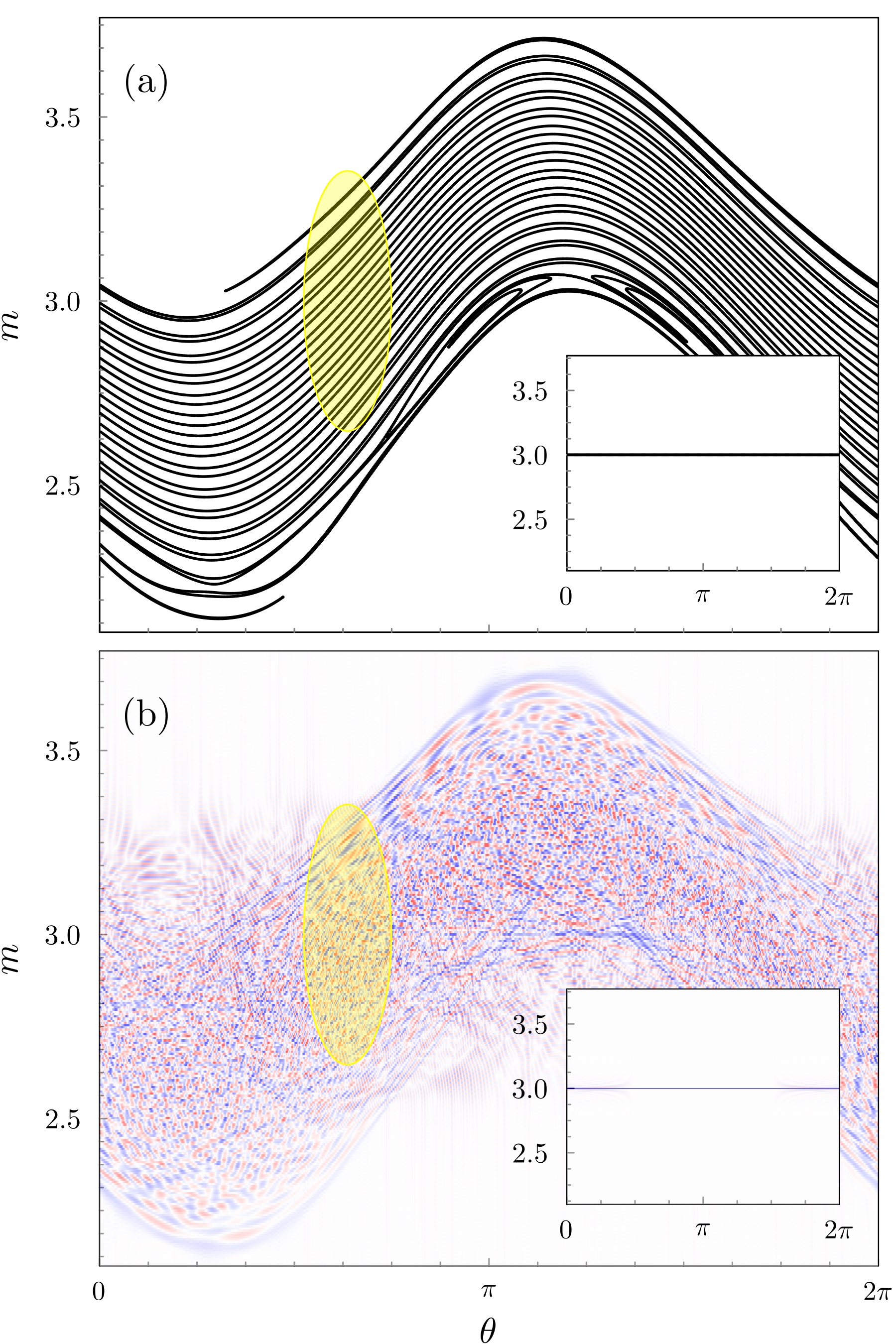
The WKB quantization of the initial Lagrangian manifold results exactly in expression (3). By iterating classically using (1), we produce an evolved Lagrangian manifold that is the exact classical counterpart of (2) with initial state (3). As an example, Fig. 1 displays a snapshot of the classical manifold (top) and the quantum Wigner function (bottom) after iterations for the KRS in the near-integrable regime. The classical mean value, which we call , is then given by substituting by a delta function with support on in (5) and is known in physics literature as the truncated Wigner approximation (e.g. [32, *polkovnikov2003quantum, *schlagheck2019enhancement]).
Following Maslov [35], our semiclassical mean value (SMV) approach is exclusively based on information contained in and is given by
| (7) |
as adapted from [24]. Here, each entering the sum represents a pair of sections of that fall inside the detector, which we denote by and . We refer to each of these sections as a filament. For each phase-space point , the coordinates are formed as the centers . The center action is given by the symplectic area of the region enclosed by the path between and on and the line segment joining and [36, 24]. Along the path on , one is expected to cross several points at which the tangent space to is parallel to the axis, which semiclassically gives rise to divergences in the representation, known as caustics [37, *littlejohn1992van, *OzorioBook]. While (7) is not impacted by them, it is fundamental to count how many were traversed in the form of a Morse index [35, 40]. Lastly, the coefficients measure how much the manifold was stretched during evolution, i.e. they can be thought of as the ratio between the length of an initial line segment in and of its image in . For a detailed discussion of these concepts, see [31].
The classical structure of Fig. 1(a) is standard for near-integrable systems: The initial manifold is stretched due to the shearing action of (1) when far from fixed points, but also captured near them, spiraling into whorls [41, 42]. The semiclassical interpretation of the oscillations seen in Fig. 1(b) is that all the branches in interfere with each other, forming the complicated patterns seen in the Wigner function. Before the so called Ehrenfest time [43], classical and quantum evolutions produce the same expectation values (that is, quantum interference cancels out when computing mean values). Since we pick a large number of kicks, we are far beyond the Ehrenfest time [43], and the classical features of Fig. 1(a) are blurred by quantum interferences in Fig. 1(b). By selecting a set of interfering branches in , detector (4) allows us to define a very objective notion of “quantumness”: the mean value is all the more quantum as more interfering segments of fall inside the detector. The number of such filaments depends mostly on the curve defining the initial state and on the dynamics of the system, but for a high degree of chaoticity it will grow exponentially with . In Fig. 1(a), for instance, there are 24 filaments within the yellow region defining 4 standard deviations of the detector.
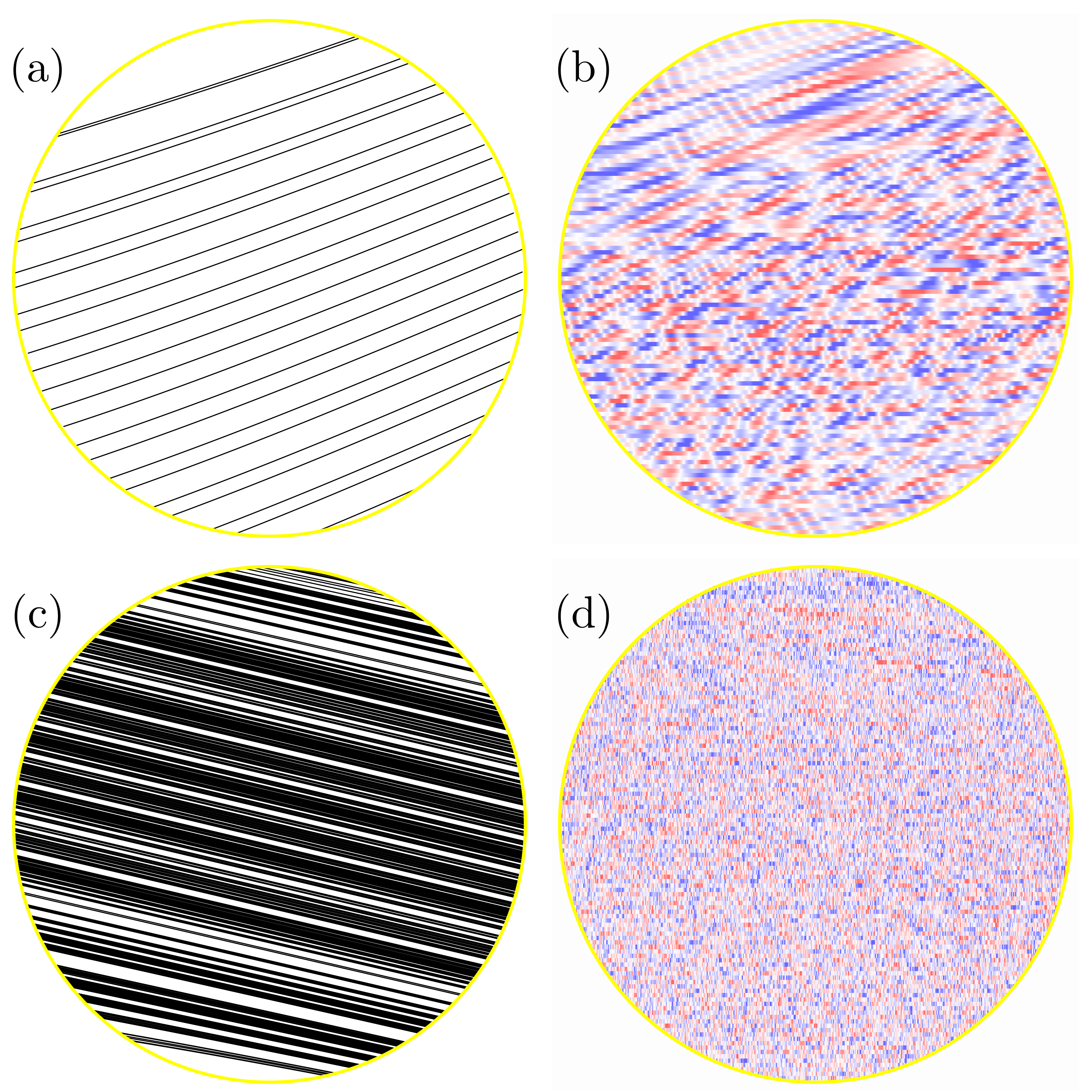
The success of a semiclassical method will depend on how accurately it is able to reproduce pairwise interferences between filaments. This task becomes harder if the number of filaments increases, which can happen by increasing either the number of kicks, , or the kicking strength, . From the detector’s point of view, the long-time (large ) semiclassical dynamics and the deeply chaotic regime (large ) are very similar, and the only important measure is the number of filaments falling inside its domain. Both limits, however, are well-known to be problematic for semiclassical mechanics [15], and producing reasonable quantitative results for a large number of filaments is a formidable task. To have a clearer idea on how intricate such a task is, in Fig. 2 we zoom in on the detector in order to have a better view of the classical and quantum structures inside it, both in the near-integrable regime of Fig. 1 and in the deep chaotic regime. The rather structured Wigner function Fig. 2(b) in the near-integrable regime, semiclassically built on top of the simple filaments of Fig. 2(a), finds an intimidating analogue in Fig. 2(d). By emerging as a result of almost one thousand interfering filaments in Fig. 2(c), the corresponding Wigner function looks ergodic and structureless.
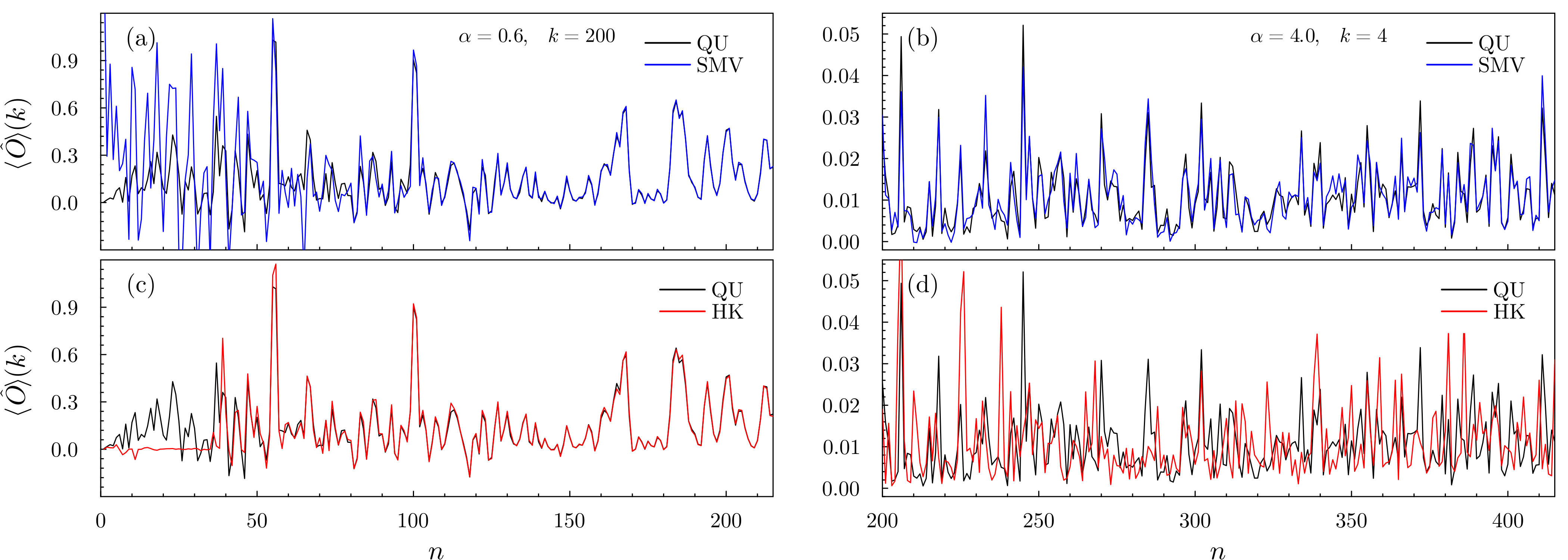
We expect a good match of both HK and SMV with the exact quantum mean values for the structure shown in Fig. 2(a). This is indeed confirmed in Fig. 3(a) and Fig. 3(c), where we plot mean values as a function of . Here, since the accuracy of semiclassical approximations improves as becomes highly oscillatory, instead of entering the semiclassical regime by increasing we define a tunable , tracking our results as a function of the integer . The advantage is that by fixing the classical dynamics is frozen. We then see that in the near-integrable regime both HK and SMV become increasingly accurate as we decrease , with the former converging earlier but being slightly less accurate for smaller values. On the other hand, in the deep-chaotic regime in Fig. 3(d) the HK calculation is essentially numerical noise, while the SMV in Fig. 3(b) displays a remarkable quantitative match with the quantum result. The result obtained from the HK method is also improved by the fact that we compute wavefunctions and only then the mean values. This allows us to renormalize the wavefunctions according to before plugging them into (5), correcting for normalization loss due to the fact that the HK propagator is not unitary. This procedure allows us to bypass one of the main flaws in the HK method, but can only be efficiently carried out for systems with a single degree of freedom. It is also important to be sure that the HK wavefunctions are properly converged before taking the mean values, and we provide extensive convergence testing in [31].
It can be argued that HK results could be improved by filtering trajectories or employing one of the many prefactor renormalization techniques developed throughout the years in computational chemistry [44, 22]. These techniques, however, are only successful when there exist regular trajectories that survive the filtering process [22]. In the deep chaotic regime phase space is completely dominated by the chaotic sea, and it is no surprise that even prefactor renormalization was not capable of improving the quality of HK calculations for the KRS – even when used in conjunction with wavefunction renormalization [45]. The fact that the HK wavefunctions are converged, yet highly inaccurate, confirms that the complexity of the classical structure in Fig. 2(c) is to blame: The HK method is simply incapable of accounting for all interfering filaments correctly. The large number of filaments, however, also leads to a combinatorial problem in a naive implementation of the SMV: Since all pairs enter (7) and the number of pairs is given by , the computational cost increases quadratically with the number of filaments, . This difficulty can be soothed by keeping in mind that not all pairs need to be included in (7), only the ones for which the action is not highly oscillatory – in practice, of . This renders the computational cost linear in the number of filaments. Our implementation also relies on filaments not developing too much structure (such as coming out from the same direction as they came in, forming a finger). This is by no means a shortcoming of the method itself, and our algorithm can be improved and adapted to particular applications as our source code is made accessible to the public [31]. For dealing with the previously mentioned fingers, for instance, a uniformization procedure in terms of Airy functions can be applied to (7) [14].
In principle, our SMV method is ready to be generalized to the propagation of coherent states, where now complex Lagrangian manifolds need to be employed [46, *tomsovic2016generalized]. An implementation for higher-dimensional systems is also possible, and will mainly imply that the intersection of the Lagrangian manifold defining our propagated state with the detector will be of dimension . Although these manifolds can be quite complicated, in the deep chaotic regime they are locally -dimensional planes, just as the filaments of Fig. 2 are essentially lines. This can extend the applicability of our method to complex chaotic systems (e.g. two- or more electron atoms), which lie beyond the applicability horizons of initial value representations such as Herman and Kluk’s. Moreover our approach can be adapted to address the dynamics of hybrid quantum-classical systems [48], or to compute other physical quantities with well-defined classical limits, such as the conductance matrix of quantum dots or the purity (linear entropy) of a bipartite quantum system.
Acknowledgements.
We thank Alfredo Ozorio de Almeida and Steven Tomsovic for fruitful discussions. The authors gratefully acknowledge support from the Grant No. ANR-17-CE300024. GML thanks Technische Universität Dresden for their hospitality and acknowledges financial support from the Institute for Basic Science in the Republic of Korea through the project IBS-R024-D1.References
- Vleck [1928] J. H. V. Vleck, The correspondence principle in the statistical interpretation of quantum mechanics, Proc. Natl. Acad. Sci. USA 14, 178 (1928).
- Einstein [1917] A. Einstein, Zum Quantensatz von Sommerfeld und Epstein, Verh. Deutsch. Phys. Ges. 19, 82 (1917).
- Holthaus and Just [1994] M. Holthaus and B. Just, Generalized pulses, Phys. Rev. A 49, 1950 (1994).
- Tannor and Garashchuk [2000] D. J. Tannor and S. Garashchuk, Semiclassical calculation of chemical reaction dynamics via wavepacket correlation functions, Annu. Rev. Phys. Chem. 51, 553 (2000).
- Brodier et al. [2001] O. Brodier, P. Schlagheck, and D. Ullmo, Resonance-assisted tunneling in near-integrable systems, Phys. Rev. Lett. 87, 064101 (2001).
- Tomsovic et al. [2018] S. Tomsovic, P. Schlagheck, D. Ullmo, J.-D. Urbina, and K. Richter, Post-Ehrenfest many-body quantum interferences in ultracold atoms far out of equilibrium, Phys. Rev. A 97, 061606(R) (2018).
- Ray et al. [2016] S. Ray, P. Ostmann, L. Simon, F. Grossmann, and W. T. Strunz, Dynamics of interacting bosons using the Herman–Kluk semiclassical initial value representation, J. of Phys. A: Math. Theo. 49, 165303 (2016).
- Lando et al. [2019] G. M. Lando, R. O. Vallejos, G.-L. Ingold, and A. M. O. de Almeida, Quantum revival patterns from classical phase-space trajectories, Phys. Rev. A 99, 042125 (2019).
- Schlagheck et al. [2022] P. Schlagheck, D. Ullmo, G. M. Lando, and S. Tomsovic, Resurgent revivals in bosonic quantum gases: A striking signature of many-body quantum interferences, Phys. Rev. A 106, L051302 (2022).
- Tomsovic and Heller [1991] S. Tomsovic and E. J. Heller, Semiclassical dynamics of chaotic motion: unexpected long-time accuracy, Phys. Rev. Lett. 67, 664 (1991).
- Tomsovic and Heller [1993] S. Tomsovic and E. J. Heller, Long-time semiclassical dynamics of chaos: The stadium billiard, Physical Review E 47, 282 (1993).
- Sieber and Richter [2001] M. Sieber and K. Richter, Correlations between periodic orbits and their rôle in spectral statistics, Physica Scripta 2001, 128 (2001).
- Heusler et al. [2007] S. Heusler, S. Müller, A. Altland, P. Braun, and F. Haake, Periodic-orbit theory of level correlations, Phys. Rev. Lett. 98, 044103 (2007).
- Berry and Mount [1972] M. V. Berry and K. Mount, Semiclassical approximations in wave mechanics, Reports on Progress in Physics 35, 315 (1972).
- Voros [1994] A. Voros, Aspects of semiclassical theory in the presence of classical chaos, Progress of Theoretical Physics Supplement 116, 17 (1994).
- Miller [2001] W. H. Miller, The semiclassical initial value representation: A potentially practical way for adding quantum effects to classical molecular dynamics simulations, J. Phys. Chem. A 105, 2942 (2001).
- Baranger et al. [2001] M. Baranger, M. A. de Aguiar, F. Keck, H.-J. Korsch, and B. Schellhaaß, Semiclassical approximations in phase space with coherent states, J. Phys. A: Math. Theor. 34, 7227 (2001).
- Kay [2005] K. G. Kay, Semiclassical initial value treatments of atoms and molecules, Annu. Rev. Phys. Chem. 56, 255 (2005).
- de Almeida et al. [2013] A. M. O. de Almeida, R. O. Vallejos, and E. Zambrano, Initial or final values for semiclassical evolutions in the Weyl–Wigner representation, J. of Phys. A: Math. Theo. 46, 135304 (2013).
- Herman and Kluk [1984] M. F. Herman and E. Kluk, A semiclasical justification for the use of non-spreading wavepackets in dynamics calculations, Chem. Phys. 91, 27 (1984).
- Lasser and Sattlegger [2017] C. Lasser and D. Sattlegger, Discretising the herman–kluk propagator, Numerische Mathematik 137, 119 (2017).
- Di Liberto and Ceotto [2016] G. Di Liberto and M. Ceotto, The importance of the pre-exponential factor in semiclassical molecular dynamics, J. Chem. Phys. 145, 144107 (2016).
- Lasser and Lubich [2020] C. Lasser and C. Lubich, Computing quantum dynamics in the semiclassical regime, Acta Numer. 29, 229 (2020).
- Mittal et al. [2020] K. M. Mittal, O. Giraud, and D. Ullmo, Semiclassical evaluation of expectation values, Phys. Rev. E 102, 042211 (2020).
- Swart [2008] T. C. Swart, Initial Value Representations (Ph.D. Thesis, F. Uni. Berlin, 2008).
- Chirikov [1979] B. V. Chirikov, A universal instability of many-dimensional oscillator systems, Phys. Rep. 52, 263 (1979).
- Note [1] Note that while the angle operator is not well defined, its exponential (and, therefore, its sine and cosine) are perfectly rigorous, which is why we place the hat over the whole sine instead of only the angle. See [49] for a nice exposition of the construction of angle and angular momentum operators.
- Lagendijk et al. [2009] A. Lagendijk, B. Van Tiggelen, and D. S. Wiersma, Fifty years of anderson localization, Phys. Today 62, 24 (2009).
- Floß et al. [2013] J. Floß, S. Fishman, and I. S. Averbukh, Anderson localization in laser-kicked molecules, Phys. Rev. A 88, 023426 (2013).
- Manai et al. [2015] I. Manai, J.-F. Clément, R. Chicireanu, C. Hainaut, J. C. Garreau, P. Szriftgiser, and D. Delande, Experimental observation of two-dimensional anderson localization with the atomic kicked rotor, Phys. Rev. Lett. 115, 240603 (2015).
- [31] See Supplemental Material, which includes references [50, 24, 49, 51, 45, 40, 52, 53], at [url will be inserted by publisher] for a comprehensive account of numerical and analytical details and a further employment of the semiclassical mean value method to the kicked harper model. the source code for computing all data presented in the paper can be found in https://github.com/gabrielmlando/meanvals., .
- Sinatra et al. [2002] A. Sinatra, C. Lobo, and Y. Castin, The truncated Wigner method for bose-condensed gases: limits of validity and applications1, J. of Phys. B 35, 3599 (2002).
- Polkovnikov [2003] A. Polkovnikov, Quantum corrections to the dynamics of interacting bosons: Beyond the truncated Wigner approximation, Phys. Rev. A 68, 053604 (2003).
- Schlagheck et al. [2019] P. Schlagheck, D. Ullmo, J. D. Urbina, K. Richter, and S. Tomsovic, Enhancement of many-body quantum interference in chaotic bosonic systems: The role of symmetry and dynamics, Phys. Rev. Lett. 123, 215302 (2019).
- Maslov and Fedoriuk [2001] V. P. Maslov and M. V. Fedoriuk, Semi-classical approximation in quantum mechanics, Vol. 7 (Springer Science & Business Media, 2001).
- De Almeida [1998] A. M. O. De Almeida, The Weyl representation in classical and quantum mechanics, Phys. Rep. 295, 265 (1998).
- Gutzwiller [1990] M. Gutzwiller, Chaos in Classical and Quantum Mechanics (Springer-Verlag, 1990).
- Littlejohn [1992] R. G. Littlejohn, The Van Vleck formula, Maslov theory, and phase space geometry, J. Stat. Phys. 68, 7 (1992).
- de Almeida [1990] A. M. O. de Almeida, Hamiltonian Systems: Chaos and Quantization, 2nd ed. (Cambridge University Press, 1990).
- Creagh et al. [1990] S. C. Creagh, J. M. Robbins, and R. G. Littlejohn, Geometrical properties of Maslov indices in the semiclassical trace formula for the density of states, Physical Review A 42, 1907 (1990).
- Berry et al. [1979] M. V. Berry, N. L. Balazs, M. Tabor, and A. Voros, Quantum maps, Ann. Phys. 122, 26 (1979).
- Berry [1979] M. V. Berry, Evolution of semiclassical quantum states in phase space, J. Phys. A. 12, 625 (1979).
- Schubert et al. [2012] R. Schubert, R. O. Vallejos, and F. Toscano, How do wave packets spread? Time evolution on Ehrenfest time scales, J. Phys. A 45, 215307 (2012).
- Walton and Manolopoulos [1996] A. R. Walton and D. E. Manolopoulos, A new semiclassical initial value method for Franck-Condon spectra, Molecular Physics 87, 961 (1996).
- Maitra [2000] N. T. Maitra, Semiclassical maps: A study of classically forbidden transitions, sub-h structure, and dynamical localization, J. Chem. Phys. 112, 531 (2000).
- Tomsovic [2015] S. Tomsovic, Generalized Gaussian wave packet dynamics for chaotic systems, Bulletin of the American Physical Society 60 (2015).
- Pal et al. [2016] H. Pal, M. Vyas, and S. Tomsovic, Generalized Gaussian wave packet dynamics: Integrable and chaotic systems, Physical Review E 93, 012213 (2016).
- Singh et al. [2022] A. Singh, L. Chotorlishvili, Z. Toklikishvili, I. Tralle, and S. Mishra, Hybrid quantum–classical chaotic NEMS, Physica D: Nonlinear Phenomena 439, 133418 (2022).
- Levy-Leblond [1976] J.-M. Levy-Leblond, Who is afraid of nonhermitian operators? A quantum description of angle and phase, Annals of Physics 101, 319 (1976).
- Arnold [1989] V. I. Arnold, Mathematical Methods of Classical Mechanics, 2nd ed. (Springer, 1989).
- Gazeau [2009] J. P. Gazeau, Coherent States in Quantum Physics (Wiley-VCH, 2009).
- Rivas and De Almeida [1999] A. Rivas and A. O. De Almeida, The weyl representation on the torus, Annals of Physics 276, 223 (1999).
- Miquel et al. [2002] C. Miquel, J. P. Paz, and M. Saraceno, Quantum computers in phase space, Physical Review A 65, 062309 (2002).