Computing Nucleon Electric Dipole Moment from lattice QCD

Observation of a non-zero nucleon electric dipole moment (nEDM) would be direct evidence for violation of CP(T)-symmetry. The Standard Model (SM) has a CP-violating phase in the CKM matrix. However, there is at least one substantial motivation to search for CP violation beyond the SM: the magnitude of the CP violation effect in CKM is insufficient to explain the observed baryon asymmetry of the universe as required by one of the famous Sakharov’s conditions for the universe’s matter origin. Currently the most sensitive probes for the CP-violating phenomena are EDM searches in hadronic, atomic, and molecular systems. The best limits on EDMs come from experiments on neutrons (ILL) [1] and ¹⁹⁹Hg [2] which constrain the nucleon EDM (nEDM) $|d_{n}|\leq 2.6\times 10^{-26}$ [$e$ cm]. This bound is $\sim 10^{5}$ larger than the prediction $\sim 10^{-31}$ [$e$ cm] from the CP phase of the CKM matrix in the SM. Observation of non-zero nEDMs would be a discovery of fundamental importance, and however, even a null result would make serious impact on cosmology and high-energy theory. Violations of CP symmetry at the quark level are represented by a number of effective quark and gluon operators. Among them, the only such renormalizable interaction is the QCD ”$\theta$-term”,

$\displaystyle iS_{\theta}=i\theta Q=i\theta\sum_{x}q(x)\,,\quad\quad q(x)=\frac{1}{16\pi^{2}}{\rm Tr}\left[G_{\mu\nu}\tilde{G}^{\mu\nu}(x)\right]$

(1)

where $Q$ is the topological charge and $q(x)$ is the topological charge density operator. Assuming that the $\theta$-term is the only source of the CP violation, we have a strong constraint on the parameter $|\theta|\lesssim 10^{-10}$. The problem of why $\theta$ is so small is known as the strong CP problem ¹¹1A dynamical solution to the strong CP problem is proposed in a parallel talk by G. Schierholz [3].. The precision of EDM measurements of nucleons and nuclei will increase in the future experiments using neutron sources, which plan to improve neutron EDMs bounds by 1-2 orders of magnitude. However, quantitative connection between magnitudes of EDMs and such CP violation operators at the quark-gluon level is very limited and model-dependent (see Refs. [4], [5] for a recent review of the EDM phenomenology). Therefore connecting the quark- and hadron-level effective interactions that include CP violating sources is an urgent task for lattice QCD.

In this proceedings, we review recent progress on the lattice calculations of the nEDM induced by the $\theta$ term. As for other CP-violating matrix elements that arise from the operators beyond the SM, these are discussed in the plenary lecture [6] ²²2See also [7] for a recent review..

In this section, we briefly review the methods for the lattice computations of the nEDM. The $\theta$-induced nEDMs have been calculated on a lattice from the CP-odd electric dipole form factor (EDFF) $F_{3}(Q^{2})$ with the $Q^{2}\to 0$ extrapolation of the nucleon matrix elements of the quark vector current [8, 9, 10, 11, 12, 13, 14, 15, 16, 17], and from nucleon energy shifts in a uniform background electric field [18, 19, 14]. The EDFF is defined as

$$\langle p^{\prime},\sigma^{\prime}|J^{\mu}|p,\sigma\rangle_{{\cancel{\rm CP}}}=\bar{u}_{p^{\prime},\sigma^{\prime}}\big{[}F_{1}(Q^{2})\gamma^{\mu}+\big{(}F_{2}(Q^{2})+iF_{3}(Q^{2})\big{)}\frac{i\sigma^{\mu\nu}q_{\nu}}{2M_{N}}\big{]}u_{p,\sigma}\,,$$

(2)

where $Q^{2}=-q^{2}$ and $q=p^{\prime}-p$, and $F_{1}$ and $F_{2}$ are the Dirac and Pauli form factors. The QCD $\theta$ term is introduced either as a modification of the lattice CP-even QCD action with imaginary $\theta$ term [10, 11] or as a Taylor expansion of nucleon correlation functions, $S_{\text{QCD}}\to S_{\text{QCD}}+iS_{\theta}$. In the latter case the nucleon-current correlation functions in ${\cancel{\rm CP}}$ QCD vacuum are modified as

$$\displaystyle\begin{aligned} \langle N\,[\bar{q}\gamma^{\mu}q]\,\bar{N}\rangle_{{\cancel{\rm CP}}}&=\frac{1}{Z}\int\,{\mathcal{D}}U\,\mathcal{D}\bar{\psi}\mathcal{D}\psi N\,[\bar{q}\gamma^{\mu}q]\,\bar{N}e^{-S-iS_{\theta}}\,\\ &=C_{NJ\bar{N}}-i\theta\,C_{NJ\bar{N}}^{Q}+O(\theta^{2})\,,\end{aligned}$$

(3)

where $C_{NJ\bar{N}}=\langle N\,[\bar{q}\gamma^{\mu}q]\,\bar{N}\rangle$ and $C_{NJ\bar{N}}^{Q}=\langle N\,[\bar{q}\gamma^{\mu}q]\,\bar{N}\,\sum_{x}[q(x)]\rangle$ are the nucleon-current correlation functions evaluated in the ${CP}$-even QCD vacuum. To obtain the EDFF $F_{3}(Q^{2})$ in Eq. (2) we have to calculate the nucleon two and three point functions

	$\displaystyle C_{\rm 2pt}^{Q}(\vec{p},t)$	$\displaystyle=\sum_{\vec{y}}e^{-i\vec{p}\cdot\vec{y}}\langle N(\vec{y},t)\bar{N}(\vec{0},0)\sum_{x}[q(x)]\rangle,$		(4)
	$\displaystyle C_{\rm 3pt}^{Q}(t,\vec{p};t_{\rm op},\vec{q})$	$\displaystyle=\sum_{\vec{y},\vec{z}}e^{-i\vec{p}\cdot\vec{y}+\vec{q}\cdot\vec{z}}\langle N(\vec{y},t)J^{\mu}(\vec{z},t_{\rm op})\bar{N}(\vec{0},0)\sum_{x}[q(x)]\rangle.$		(5)

In general the nucleon ground states as well as their overlaps with the positive-parity nucleon ground state are modified in ${\cancel{\rm CP}}$ QCD vacuum as

$\displaystyle\langle 0|N|p,\sigma\rangle_{\cancel{\rm CP}}=Z_{N}e^{i\alpha\gamma_{5}}u_{p,\sigma}=Z_{N}\tilde{u}_{p,\sigma},$

(6)

where $\tilde{u}_{p,\sigma}$ is a spinor wave function for the nucleon state $|p,\sigma\rangle_{\cancel{\rm CP}}$ and $Z_{N}$ is a normalization constant. The spinor $\tilde{u}_{p,\sigma}$ satisfies the following free Dirac equation with CP-violating $\gamma_{5}$ mass

$\displaystyle({\ooalign{\hfil/\hfil\crcr$p$}}-m_{N}e^{-2i\alpha\gamma_{5}})\tilde{u}_{p,\sigma}=({\ooalign{\hfil/\hfil\crcr$p$}}-m_{N}e^{-2i\alpha\gamma_{5}})e^{i\alpha\gamma_{5}}u_{p,\sigma}=0,$

(11)

where $u_{p,\sigma}$ is a wave function spinor in CP-even QCD vacuum. Thus when the CP violating effect exists in the QCD vacuum, one should use the modified nucleon spinor $\tilde{u}_{p,\sigma}$ in lattice calculations which affects the kinematic coefficients. For example, ignoring excite states, the nucleon two-point correlation function with CP violating operator can be represented as

$\displaystyle C_{\rm 2pt}^{Q}(\vec{p},t)$

$\displaystyle=|Z_{N}|^{2}\frac{e^{-E_{p}t}}{2E_{p}}\sum_{\sigma}\tilde{u}_{p,\sigma}\bar{\tilde{u}}_{p,\sigma}=|Z_{N}|^{2}\frac{e^{-E_{p}t}}{2E_{p}}\left(m_{N}e^{2i\alpha\gamma_{5}}-i{\ooalign{\hfil/\hfil\crcr$p$}}\right),$

(14)

where we use the completeness condition for the free Dirac spinor,

$\displaystyle\sum_{\sigma}\tilde{u}_{p,\sigma}\bar{\tilde{u}}_{p,\sigma}=e^{i\alpha\gamma_{5}}\left(\sum_{\sigma}u_{p,\sigma}\bar{u}_{p,\sigma}\right)=m_{N}e^{2i\alpha\gamma_{5}}-i{\ooalign{\hfil/\hfil\crcr$p$}}.$

(17)

The modification also affects the nucleon matrix elements $\langle p^{\prime},\sigma^{\prime}|J^{\mu}|p,\sigma\rangle_{\cancel{\rm CP}}$ as

	$\displaystyle\bar{\tilde{u}}_{p^{\prime},\sigma^{\prime}}\left[\tilde{F_{1}}\gamma^{\mu}+(\tilde{F_{2}}+i\tilde{F_{3}}\gamma_{5})\frac{i\sigma^{\mu\nu}q_{\nu}}{2m_{N}}\right]\tilde{u}_{p,\sigma}$	$\displaystyle=\bar{u}_{p^{\prime},\sigma^{\prime}}\left[\tilde{F_{1}}\gamma^{\mu}+e^{2i\alpha\gamma_{5}}(\tilde{F_{2}}+i\tilde{F_{3}}\gamma_{5})\frac{i\sigma^{\mu\nu}q_{\nu}}{2m_{N}}\right]u_{p,\sigma}$
		$\displaystyle=\bar{u}_{p^{\prime},\sigma^{\prime}}\left[F_{1}\gamma^{\mu}+(F_{2}+iF_{3}\gamma_{5})\frac{i\sigma^{\mu\nu}q_{\nu}}{2m_{N}}\right]u_{p,\sigma}.$

In the original lattice calculation [8], while the CP violation effect on the kinematic coefficient in Eq. (17) have been correctly taken into account, the inadequate definition of these form factors of $\tilde{F}_{1,2,3}$ has been used prior to [14]. As a result, all previous lattice results has a spurious contributions to the EDFF computed with $\tilde{F}_{3}$ from the Pauli form factor $F_{2}$ as

$\displaystyle\tilde{F_{3}}=F_{3}-2\alpha F_{2}.$

(18)

Thus if the ”Old” formula ($\tilde{F_{3}}$) is used for extracting the nEDM $\tilde{d}_{n}=\tilde{F}_{3}(0)/(2m_{N})$, there is a correction from the spurious mixing, which becomes significant when $\alpha$ becomes large.

The inconsistency between ”Old” and ”New” formula can be directly and numerically confirmed by comparing with computing nEDM from the energy shift method. The uniform electric field that preserves translation invariance and the (anti-) periodic boundary conditions on a lattice was first introduced in [20] to study the nEDM, and also applied to CP-even quantities such as electric polarizability and magnetic moments of the nucleon [21, 22]. The uniform background electric field is analytically continued to an imaginary value, so that the nucleon energy shift due to nEDM becomes imaginary. Expanding the two-point function up to the first order in $\theta$ we can directly extract the nEDM contribution that is linear in $t$. For simplicity we only consider the neutral particles, since the correlation function of charged particles is more complicated. To introduce the background electric field we consider the following Euclidean $U(1)$ vector potential

$\displaystyle A_{x,j}=n_{ij}\Phi_{ij}x_{i},\quad\quad A_{x,i}|_{x_{i}=L_{i}-1}=-n_{ij}\Phi_{ij}L_{i}x_{j},$

(19)

where $\Phi_{\mu\nu}=\frac{6\pi}{L_{\mu}L_{\nu}}$ is the quantum field flux on a plaquette ($\mu\nu$) and $n_{\mu\nu}$ is the corresponding number of quanta. The (anti-) periodicity on a lattice in both space and time requires the Dirac quantization conditions

$\displaystyle Q_{q}\Phi_{\mu\nu}L_{\mu}L_{\nu}=2\pi n_{\mu\nu},\quad\quad\left(Q_{u}=\frac{2}{3},\ \ Q_{d}=-\frac{1}{3}\right)$

(20)

The electric field vector is then given as $\vec{E}=(n_{14}\Phi_{14},n_{24}\Phi_{24},n_{34}\Phi_{34})$. The corresponding effective Dirac equation for nucleon field $\tilde{N}$ is given as

$\displaystyle\left({\ooalign{\hfil/\hfil\crcr$p$}}-(\tilde{\kappa}+i\tilde{\zeta}\gamma_{5})\frac{F_{\mu\nu}}{2}\frac{\sigma^{\mu\nu}}{2m_{N}}-m_{N}e^{-2i\alpha\gamma_{5}}\right)\tilde{N}=0,$

(23)

where $\tilde{\kappa}=\tilde{F}_{2}(0)$ and $\tilde{\zeta}=\tilde{F}_{3}(0)$ are the effective anomalous magnetic and electric moments in the basis of $\tilde{N}$ with $\gamma_{5}$ mass. It is obvious that the ${\cancel{\rm CP}}$ phase $e^{i\alpha\gamma_{5}}$ can be completely rotated away by a field redefinition $N=e^{i\alpha\gamma_{5}}\tilde{N}$, where the two couplings also transform $e^{2i\alpha}(\tilde{\kappa}+i\tilde{\zeta})=(\kappa+i\zeta)$. Considering an electric field in $z$-direction $\vec{E}=(0,0,E_{z})$ in the rest frame $p^{\mu}=(\vec{0},E_{s})$, we obtain an on-shell solution spinor $u_{E_{z},s}$ for the spin polarized along $z$-direction with $s=\pm$, which has a spin-dependent energy eigenvalue $E_{s}=m_{N}-\frac{\zeta}{2m_{N}}(sE_{z})+O(E_{z}^{2})$. From the result we see that the resulting energy shift is consistent with the EDFF obtained in the basis of $N$ without $\gamma_{5}$ mass, and $\kappa=F_{2}(0)$ and $\zeta=F_{3}(0)$ are the nucleon magnetic and electric dipole moment coefficients. By taking the analytic continuation of the electric field $E_{z}$ to the imaginary value we obtain the energy shift of a nucleon on lattice as $\tilde{E}_{\pm}=m_{N}\pm\delta E$, with $\delta E=-\zeta/(2m_{N})iE_{z}$. To extract the nucleon energy shift we calculate the following nucleon two point functions in the presence of the background electric fields

$\displaystyle C_{{\rm 2pt},\vec{E}}^{Q}(\vec{p},t)=\sum_{\vec{y}}e^{-i\vec{p}\cdot\vec{y}}\langle N(\vec{y},t)|\bar{N}(\vec{0},0)\sum_{x}[q(x)]\rangle_{\vec{E}}.$

(24)

Using the solution spinor $u_{E_{z},s}$ and ignoring excited states we can expand $C_{{\rm 2pt},\vec{E}}^{Q}(\vec{p},t)$ as

	$\displaystyle C_{{\rm 2pt},\vec{E}}^{Q}(\vec{0},t)$	$\displaystyle=|Z_{N}|^{2}\sum_{s=\pm}\tilde{u}_{E_{z},s}\bar{\tilde{u}}_{E_{z},s}\frac{e^{-\tilde{E}_{s}t}}{2\tilde{E}_{s}}$
		$\displaystyle=|Z_{N}|^{2}\left[\frac{1+\gamma_{4}}{2}(1-\Sigma^{z}\delta Et)+i\alpha_{5}\gamma_{5}+\Sigma^{z}\frac{\kappa E_{z}}{2m^{2}}\gamma_{5}\right]e^{-m_{N}t}+O(\delta E^{2},E_{z}^{2}),$		(25)

where $\Sigma_{z}=-i\gamma_{x}\gamma_{y}$. Using the standard ratio method we define an “effective” energy shift $\zeta_{n}^{\rm eff}(t)=2m_{N}d_{n}=\frac{-2m_{N}}{E_{z}}(R(t+1)-R(t))$, and $R(t)$ is defined as a ratio of two-point functions with two different spin projections

$\displaystyle R(t)=\frac{{\rm Tr}[(T_{S_{z+}}-T_{S_{z-}})C_{{\rm 2pt},\vec{E}}^{\cancel{\rm CP}}(\vec{0},t)]}{2{\rm Tr}[T_{p}C_{{\rm 2pt},\vec{E}}^{\cancel{\rm CP}}(\vec{0},t)]},$

(26)

where we use spin polarization projection operators $T_{S_{z\pm}}=\frac{1+\gamma_{4}}{2}(1\pm\Sigma_{z})$, and $T_{p}=(1+\gamma_{4})$. Thus the nEDM in the energy shift method is independent from the parity mixing ambiguity, from which we numerically verify the consistency with the “New” formula ($F_{3}$). For more detail on the analyses, see Ref. [14].

We show some nEDM results in comparison between the form factors and the energy shift methods. Fig. 2 shows how the spurious mixing affects the result for the $\theta$-EDM. As shown in the figure, the magnitudes of $F_{3}(Q^{2})$ with ”New” are smaller than the ”Old” values. We also show the result for nEDM $\zeta_{n}^{\rm eff}$ computed from the effective energy shift in Fig. 2, where we computed with two values of flux quanta $n=n_{34}=\pm 1$ and $\pm 2$. A plateau for the effective energy $\zeta_{n}^{\rm eff}$ at $t=4\sim 7$ can be obtained in both electric fields of $|n|=1$ and $2$. Comparing the form factor method we obtain a consistent result only if we use the “New” formula. This result is also consistent with naively corrected data using the previously reported values prior to [14]. Since we obtain a small but non-zero signal $|d_{n}^{\theta}|\lesssim 0.1\frac{e}{2m_{N}}$ at $m_{\pi}=330$ MeV, we estimate an extrapolated value to the physical point based on a naive scaling of the ChPT expectation $d_{n}\sim m_{q}\sim m_{\pi}^{2}$, which suggests that the signal becomes weaker as the quark mass is approaching to the physical point and we would obtain a smaller value of $|d_{n}^{\theta}(m_{\pi}^{\rm phys})|\lesssim 0.02\frac{e}{2m_{N}}$. From our findings in order to promote a direct calculation of nEDM at the physical point, various noise reduction techniques that work in particular for gluon operator are required in addition to a significant increase in statistics.

As explained in the previous section, $\theta$-induced nEDM would be extremely challenging in the physical point, because the topological charge fluctuation dominates the large statistical noise growing with lattice volume $V_{4}$ as $\delta Q^{2}=\langle Q^{2}\rangle\propto V_{4}$, while the signal becomes small. Since the global topological charge is zero on average because our QCD action is CP-even, $F_{3}(Q^{2})$ is the signal of the correlation between the gluon operator and the fermionic (nucleon) functions as shown in Eq. (5). Thus it has been originally suggested that truncation of the topological charge sum at a large distance from the nucleon position can reduce fluctuations of the nEDM [13] (also known as a cluster decomposition of disconnected diagrams [23]), since contributions of $Q$ at large distance may be neglected in computing the nEDM, while its correlation has a large noise which is not suppressed with space-time distance due to the global nature of the topological charge. To extend this method, in Ref. [24] we consider a generalized reduced topological charge density which separately restrict time and space to a cylindrical volume $V_{Q}$,

$\displaystyle\tilde{Q}(\Delta t_{Q},r_{Q})=\frac{1}{16\pi^{2}}\sum_{x\in V_{Q}}{\rm Tr}\big{[}\hat{G}_{\mu\nu}\tilde{\hat{G}}_{\mu\nu}\big{]}_{x}\,,\quad(\vec{x},t)\in V_{Q}:\left\{\begin{array}[]{l}|\vec{x}-\vec{x}_{0}|\leq r_{Q}\,,\\ t_{0}-\Delta t_{Q}<t<t_{0}+t_{\rm sep}+\Delta t_{Q}\,,\end{array}\right.$

(29)

where $t_{0}$ and $t_{0}+t_{\rm sep}$ are the positions of the nucleon source and sink. This setup is illustrated in Fig. 3, where the three-point functions are inside entirely the region $V_{Q}$ and the truncation in $t$-direction for $\tilde{Q}$ is symmetric with respect to the nucleon sources and sinks for both two- and three-point functions. We also set $\vec{x}_{0}$ to the nucleon source position to further reduce the noise at large distances. We should note that a spatial restriction may introduce another bias for nEDM. In order to avoid such ambiguity, the convergence with $r_{Q}$ and $\Delta t_{Q}$ in Eq. (29) must be verified at each nucleon momenta, especially in computing the $Q^{2}$ dependence of the EDFFs.

We use the lattice QCD ensemble of dynamical domain wall fermion with heavy pion mass $m_{\pi}=330$ MeV. We calculate 64 low-precision and 1 high-precision samples using the AMA sampling method [25]. The topological charge density is calculated using the “5-loop-improved” field strength $\hat{G}_{\mu\nu}$ [26] with the gradient flow ($t_{gf}=8a^{2}$). The $r_{Q}$ and $\Delta t_{Q}$ dependence of the mixing angle $\alpha$ and the EDFF for the neutron (connected diagram only) are shown in Figs. 4 and 5, where we observe error reduction for smaller values of $r_{Q}$ and $\Delta_{Q}$ and convergence for $r_{Q}\geq 16$, $\Delta t_{Q}\geq 8$ in both $\alpha$ and $F_{3}(Q^{2})$. We have also performed a calculation using ensembles at the physical point on $48^{3}\times 96$ lattice with 33,000 statistics. Unfortunately we have found no signal for neutron EDFFs (See Fig. 6), and the results are consistent with zero with the statistical uncertainty. Our result of signal-to-noise ratio $\sim 0.2$ at $m_{\pi}=330$ MeV indicates that the expected signal-to-noise ratio at the physical point has to be improved by a factor of $\sim$10 which requires $\times O(100)$ more statistics to confirm the existence of the strong CP problem.

A systematic analysis of the truncation method based on spectrum decomposition is proposed in Refs. [15, 16]. This study uses a truncation of the topological charge density operator summed over spatial directions $\bar{Q}$ defined as

$\displaystyle\bar{Q}(t_{Q})=\int d^{3}xq(x,t_{Q}),\quad\quad q(x,t_{Q})=\frac{1}{16\pi^{2}}G\tilde{G}(x,t_{Q})$

(30)

where the topological charge density $q(x,t_{Q})$ is again calculated using the gradient flow method. To calculate the nucleon mixing angle, the following modified two-point function

$\displaystyle\Delta C_{\rm 2pt}(t,t_{Q})=\langle{\rm T}\{N(T)\bar{Q}(t_{Q})\bar{N}(0)\}\rangle,$

(31)

is considered. The spectrum decomposition for $\Delta C_{\rm 2pt}(t,t_{Q})$ reveals its $t_{Q}$ dependence and provide a systematic way to estimate the truncation error. For example, in the case of $0<t_{Q}<t$, its spectral decomposition has the form

	$\displaystyle\Delta C_{\rm 2pt}(t,t_{Q})=\langle N(t)\bar{Q}(t_{Q})\bar{N}(0)\rangle$	$\displaystyle\sim\sum_{n,m}e^{-E_{n}(t-t_{Q})-E_{m}t_{Q}}\langle 0|N|n\rangle\langle n|\bar{Q}|m\rangle\langle m|\bar{N}|0\rangle$
		$\displaystyle\sim\sum_{m\neq n}\cosh{\left(\Delta m_{mn}(t_{Q}-t/2)\right)},$		(32)

where $\Delta_{mn}=E_{m}-E_{n}$. Note that two states of $n$ and $m$ should have different intrinsic parities, otherwise the contribution vanishes since the matrix element should be zero, e.g., $\langle n|\bar{Q}|n\rangle=0$ in CP-even QCD vacuum if $n$ has even or odd parity. On the other hand, in the case of $t<t_{Q}$, it has

	$\displaystyle\Delta C_{\rm 2pt}(t,t_{Q})=\langle\bar{Q}(t_{Q})N(t)\bar{N}(0)\rangle$	$\displaystyle\sim\sum_{n,m}e^{-E_{n}t_{Q}-E_{m}t}\langle 0|\bar{Q}|n\rangle\langle n|N|m\rangle\langle m|\bar{N}|0\rangle$
		$\displaystyle\sim\sum_{n^{\prime}}e^{-E_{n^{\prime}}t_{Q}},$		(33)

where the state $n^{\prime}$ should be a P-odd state that couples to a nucleon state with a non-zero value of the matrix element $\langle 0|\bar{Q}|n^{\prime}\rangle\neq 0$. From the spectrum decomposition we see that the nucleon mixing angle $\alpha$ is a mixing parameter between the ground state nucleon and CP-odd excited states. To see the truncation artefacts, the authors of Refs. [15, 16] consider the partial summed two-point correlation function $\displaystyle C^{\bar{Q}}_{\rm 2pt}(t_{s})=\sum_{t_{Q}=-t_{s}}^{t_{s}}\Delta C_{\rm 2pt}(t,t_{Q})$. From Eqs. (3) and (3) its asymptotic form behaves like $\displaystyle C^{\bar{Q}}_{\rm 2pt}(t_{s})=A+Be^{-Et_{s}}$ for $t_{s}\gtrsim t$, where the contribution for large $t_{s}$ is expected to be exponentially suppressed. This is numerically checked as shown in the left panel of Fig. 7, where a plateau is obtained for $t_{s}\sim t$ and the contributions from $t_{s}>t$ seem to be below the statistical fluctuation. Neglecting unnecessary noise from $t_{s}\gtrsim t$, an improvement of $\alpha$ up to a factor 2 is obtained. The same spectrum decomposition can be applied to the modified nucleon three point function $\Delta C^{\bar{Q}}_{\rm 3pt}(t,t_{Q},t_{\rm op})=\langle{\rm T}\{N(T)J^{\mu}(t_{\rm op})\bar{Q}(t_{Q})\bar{N}(0)\}\rangle$, where a fit analysis using its asymptotic form with the $\alpha$-improvement yields a factor of $2\sim 3$ times increases in the signal-to-noise ratio for EDFF $F_{3}(Q^{2})$. The right panel of Fig. 7 shows a chiral (and continuum) extrapolation for $d_{n}^{\theta}$ using six ensembles with $m_{\pi}>410$ MeV for several lattice spacings. A ChPT fit ansatz $d_{n}^{\theta}\sim m_{q}\sim m_{\pi}^{2}$ is used to further constrain the nEDM towards the chiral limit, which yields $d_{n}^{\theta}=-0.00152(71)\theta$ $e$ fm at the physical point with $\sim$ 2 $\sigma$ deviation from zero. This result is consistent with the aforementioned naively scaled value $|d_{n}^{\theta}(m_{\pi}^{\rm phys})|\lesssim 0.02\frac{e}{2m_{N}}$ [24]. Their fitted data, however, are in heavy pion mass region and do not clearly show the chiral behavior $d_{n}^{\theta}\propto m_{\pi}^{2}$, so that the fit results seem to be less convincing. To avoid model dependence, more accurate results near the physical point are needed.

New results near the physical point ($m_{\pi}=130$-$310$ MeV) are presented in a parallel talk by Boram Yoon [17]. The topological charge is calculated using the $O(a^{4})$-improved field strength [27] with the gradient flow on MILC HISQ ensembles with $a=0.06-0.15$ fm. This study also uses the truncation method in $t$-direction. While the convergence properties in partial sum can be seen in both two- and three- point functions, due to the slow convergence at the physical point no significant improvement is observed. It is, however, remarkable that the number of measurements is $O$(100k), which gives a statistically significant signal for $F_{3}(Q^{2})$ with non-zero $Q^{2}$ near the physical point (see the left panel of Fig. 8). It is also reported that a variance reduction technique introduced in [28] has about $25$% error reduction. In this calculation the excited state contamination is removed by using the two-state fits with multiple source-sink separations for each momentum $Q^{2}$. The results for $F_{3}(Q^{2})$ at heavier $m_{\pi}$ with non-zero $Q^{2}$ are consistent with the previous lattice results [24, 16]. The result from the chiral (interpolation) and continuum extrapolation fit for $d_{n}^{\theta}$ are also presented in the right panel of Fig. 8, which yields a non-zero signal of $|d_{n}^{\theta}|=0.011(6)\theta$ $e$ fm at the physical point. While this result is also consistent with estimates from ChPT analysis and the QCD sum rules [4], it is not sufficient to constrain the $\theta$ parameter. We also notice that even though the values of $d_{n}^{\theta}$ at finite $a$ are all positive except for the data at $m_{\pi}=135$ MeV, these values in the continuum limit become negative, which may indicate a sizable discretization effect on $d_{n}^{\theta}$. In addition, there is an increasing tendency of $F_{3}(Q^{2})$ towards $Q^{2},m_{\pi}^{2}\to 0$ but with larger error. A leading order ChPT fit may not be suitable for $d_{n}^{\theta}$ in the simulation mass region, and understanding the $Q^{2}$ dependence of $F_{3}(Q^{2})$ would be important to precisely determine $d_{n}^{\theta}$ at the physical point.

We have shown in this section that there are several ongoing studies of the $\theta$-induced nEDM. Even having $O$(100k) statistics with employing noise reduction techniques at the physical point, it still is not sufficient to constrain the $\theta$ parameter due to the large fluctuation of the topological charge density, which should become even worse when approaching to the continuum and larger volume limit. There also are several systematic uncertainties due to finite lattice spacing and $Q^{2}\to 0$ extrapolation in EDFF $F_{3}(Q^{2})$, which need to be further explored. Thus $\theta$-induced EDM at the physical point will be extremely challenging and will require more special techniques that work well in particular for gluon operators. In the next section, we would like to propose a new approach using a matrix element of the nucleon with background electric field. Since this approach is based on the energy shift method, we can directly obtain $d_{n}^{\theta}$ without $Q^{2}$ extrapolation, which may be potentially advantageous over the form factor method.

The idea is to simply apply the truncation technique to the energy shift method in the presence of the background electric field, in which we find that the energy shift $\delta E$ in Eq. (25) is given as a nucleon matrix element of the topological charge density operator $\bar{Q}$ in Eq. (30). Throughout the section, the state’s momenta are set to zero and arguments of $\vec{p}$ are suppressed. Performing the spectrum decomposition of $\Delta C_{\rm 2pt}(t,t_{Q})$ as in Eq. (3) but now in the presence of the background electric field, we obtain the following result for $t>t_{Q}$ as

	$\displaystyle\Delta C_{{\rm 2pt},\vec{E}}(t,t_{Q})$	$\displaystyle=\langle N(t)\bar{Q}(t_{Q})\bar{N}(0)\rangle_{\vec{E}}$
		$\displaystyle=\sum_{n,m}e^{-E_{n}(t-t_{Q})-E_{m}t_{Q}}\langle 0|N|n,\vec{E}\rangle\langle n,\vec{E}|\bar{Q}|m,\vec{E}\rangle\langle m,\vec{E}|\bar{N}|0\rangle$
		$\displaystyle\sim|Z_{N_{+}}|^{2}e^{-m_{N_{+}}t}\langle N_{+},\vec{E}|\bar{Q}|N_{+},\vec{E}\rangle,$		(34)

where $|N_{+},\vec{E}\rangle$ is the ground state nucleon in the presence of the background electric field. We should note that in contrast to Eq. (3), there is a leading order contribution from the ground state nucleon given as a matrix element $\langle N_{+},\vec{E}|\bar{Q}|N_{+},\vec{E}\rangle$. Again taking the partial summation of $\Delta C_{{\rm 2pt},\vec{E}}(t,t_{Q})$ over sink-source separation $t$, we obtain

$\displaystyle C_{{\rm 2pt},\vec{E}}^{\bar{Q}}(t)=\sum_{t_{Q}=0}^{t}\Delta C_{{\rm 2pt},\vec{E}}(t,t_{Q})\sim|Z_{N_{+}}|^{2}e^{-m_{N_{+}}t}(t\langle N_{+},\vec{E}|\bar{Q}|N_{+},\vec{E}\rangle),$

(35)

where the matrix element is given the coefficient of linear in $t$. Comparing Eq. (25) with Eq. (35), we find that the matrix element should correspond to the energy shift

$\displaystyle\langle N_{+},\vec{E}|\bar{Q}|N_{+},\vec{E}\rangle=-\frac{\zeta}{2m_{N}}\bar{u}\left[\vec{\Sigma}\cdot\vec{E}\right]u+O(\vec{E}^{2}).$

(36)

This formula is analogous to the leading order energy correction in the perturbation theory of quantum mechanics, c.f., $\Delta E_{n}=\langle n|\Delta\hat{H}|n\rangle$ for Hamiltonian $\hat{H}=\hat{H}_{0}+\Delta\hat{H}$. In this case we regard the electric field as a perturbation in addition to the CP-odd Hamiltonian ($\theta$-term), and also take into account a leading order perturbation effect on the state $|N_{+},\vec{E}\rangle$. Even without $\theta$-term, the ground state $|N_{+},\vec{E}\rangle$ could mix with CP-odd states [29] due to the background electric field as

$\displaystyle|N_{+},\vec{E}\rangle$

$\displaystyle=|N_{+}\rangle+c\vec{E}\cdot\vec{D}|N_{-}\rangle+\cdots,$

(37)

where $|N_{+}\rangle$ is the parity-even ground state nucleon in (lattice) CP-even vacuum. The leading order correction should come from a parity-odd nucleon $|N_{-}\rangle$ with an overlap coefficients of $c$ and the electric field $\vec{E}$ and an expectation value of the dipole operator $\vec{D}$  [29]. Substituting Eq. (37) into Eq. (36), we obtain

$\displaystyle\langle N_{+},\vec{E}|\bar{Q}|N_{+},\vec{E}\rangle$

$\displaystyle=\vec{E}\cdot\vec{D}\langle N_{+}|\bar{Q}|N_{-}\rangle+({\rm c.c.})+\cdots,$

(38)

where we note $\langle N_{\pm}|\bar{Q}|N_{\pm}\rangle=0$ due to parity symmetry, since we consider the electric field as a perturbation so that $|N_{\pm}\rangle$ is defined in CP-even QCD vacuum. Thus the contribution of the matrix element $\langle N_{+}|\bar{Q}|N_{-}\rangle$ is exactly the same as the parity mixing effect that appears in calculation of $\alpha$ in Eq. (3). In the perturbation theory point of view, the EDM is an interplay of the electric field and the CP-odd operator both in the first order perturbation. Using the standard ratio method as in Eq. (26) and the relation to the matrix element in Eq. (36), we obtain the modified energy shift formula

$\displaystyle R_{S_{z\pm}}(t,t_{Q})=\frac{{\rm Tr}[T_{S_{z\pm}}\Delta C_{{\rm 2pt},\vec{E}}(t,t_{Q})]}{{\rm Tr}[T_{p}C_{2pt,\vec{E}}(t)]}\to\mp\frac{\zeta}{2m_{N}}E_{z},\quad\quad(t\to\infty),$

(39)

From this formula, it is clear that we do not need to extend $t_{Q}$ outside the sink-source position, since there is no other term that is proportional to $t$ in $t_{Q}>t$. In fact the contributions from $t_{Q}>t$ should be excited state contaminations that should disappear in the limit $t\to\infty$. Thus, without $Q^{2}$ extrapolation, the EDFF $F_{3}(0)$ can be directly extracted from the ratio by dividing by the electric field as $\displaystyle|F_{3}(0)|=\lim_{t\to\infty}\frac{2m_{N}|R_{S_{z\pm}}(t,t_{Q})|}{|E_{z}|}$.

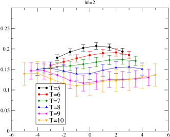
We show our preliminary results on the $\theta$-induced nEDM from the matrix element approach. Since we compute the matrix element with the electric fields along $z$-direction in both positive and negative, we have four results for each component of $\pm E_{z}$ and projections $T_{S_{z\pm}}$ (see Fig. 9). Obviously these data are correlated with each other and differences between spin up (or positive $E_{z}$) and spin down (or negative $E_{z}$) reduce the error. Fig. 10 shows the gradient flow time $t_{gf}$ dependence of $F_{3}(0)$ for each sink-source time separation $t=T$. As expected, the signal becomes better as increasing the flow time, and the result for $F_{3}(0)$ becomes stable at $t_{gf}\geq 4$ and $T\geq 8$. We also study a possible higher order correction in $\vec{E}$. Fig. 11 shows the comparison of two results for $F_{3}(0)$ with different electric field strength with $|n|=1$ and $2$, where both results $|n|=1$ and $2$ are consistent with each other for $T\geq 8$, This result indicates that $O(\vec{E}^{2})$ corrections on $F_{3}(0)$ are small. From the plateau at $T=9$ with $t_{gf}=8$ we obtain $F_{3}(0)=0.12(3)$ for the neutron at $m_{\pi}=330$ MeV. Our result seems to be consistent with the previous result obtained in the form factor method (see e.g., Fig. 8) while our value is only available at $Q^{2}=0$ and not directly comparable with the previous results.

Lattice calculations of nEDM are important for interpreting CP-violation effects in EDM experiments and cosmological observations. A number of groups are putting in the effort required for computing nEDM at the physical point using the form factor method. The nEDM induced by $\theta$-term has a large statistical noise in its correlation to the topological charge density, which is not suppressed at a large distance due to its global nature. To reduce the error several noise reduction techniques using the truncation of (space and) time region of the topological charge density have been employed. It is found that while the truncation reduces the error by a factor of 2 at a heavier pion mass, due to its poor convergence no significant improvement is observed at the physical pion mass. There also are several systematic uncertainties in $F_{3}(Q^{2})$. The uncertainties of the discretization effect, $Q^{2}\to 0$ extrapolation, and excited state contamination for $F_{3}(Q^{2})$ have not been well understood, which seem to become significant near the physical point. To control the systematic errors and to further improve the statistical signal, we have proposed a new approach using the matrix element with background electric fields. This method only requires a local topological charge density operator between sink and source positions, and thus can avoid the large topological noise at a large distance. In addition, no $Q^{2}$ extrapolation is required since the forward matrix element is directly obtained from the energy shift. Our preliminary results have demonstrated that we can achieve statistically-significant signal at heavier pion masses that are consistent with the previous results. This method can in principle be applied to any ${\cancel{\rm CP}}$ operators, in which the Weinberg’s three-gluon operator especially is beneficial for this method, since there is no additional computation cost for the gluonic operator. We need further investigations at the physical point.

The speaker would like to thank the organizers of Lattice2019 in Wuhan for the invitation. We would also like to thank Tanmoy Bhattacharya and Boram Yoon for sending us their materials and the fruitful discussions. We are grateful for the gauge configurations provided by the RBC/UKQCD collaboration. This research used resources of the Argonne Leadership Computing Facility, which is a DOE Office of Science User Facility supported under Contract DE-AC02-06CH11357, and Hokusai supercomputer of the RIKEN ACCC facility. H.O. is supported in part by JSPS KAKENHI Grant Numbers 17K14309 and 18H03710. S.S. is supported by the National Science Foundation under CAREER Award PHY-1847893.

References

- [1] C. A. Baker et al., “An Improved experimental limit on the electric dipole moment of the neutron,” Phys. Rev. Lett. 97, 131801 (2006) doi:10.1103/PhysRevLett.97.131801 [hep-ex/0602020].
- [2] B. Graner, Y. Chen, E. G. Lindahl and B. R. Heckel, “Reduced Limit on the Permanent Electric Dipole Moment of Hg199,” Phys. Rev. Lett. 116, no. 16, 161601 (2016) Erratum: [Phys. Rev. Lett. 119, no. 11, 119901 (2017)] doi:10.1103/PhysRevLett.119.119901, 10.1103/PhysRevLett.116.161601 [arXiv:1601.04339 [physics.atom-ph]].
- [3] Y. Nakamura and G. Schierholz, arXiv:1912.03941 [hep-lat].
- [4] J. Engel, M. J. Ramsey-Musolf and U. van Kolck, “Electric Dipole Moments of Nucleons, Nuclei, and Atoms: The Standard Model and Beyond,” Prog. Part. Nucl. Phys. 71, 21 (2013) doi:10.1016/j.ppnp.2013.03.003 [arXiv:1303.2371 [nucl-th]].
- [5] N. Yamanaka, “Review of the electric dipole moment of light nuclei,” Int. J. Mod. Phys. E 26, no. 4, 1730002 (2017) doi:10.1142/S0218301317300028 [arXiv:1609.04759 [nucl-th]].
- [6] T. Bhattacharya, R. Gupta, B. Yoon, ”Recent results of nucleon strucutre & matrix element calculations” Proceedings of Sciece, LATTICE2019 (2020), p.247.
- [7] R. Gupta, “Present and future prospects for lattice QCD calculations of matrix elements for nEDM,” PoS SPIN 2018, 095 (2019) doi:10.22323/1.346.0095 [arXiv:1904.00323 [hep-lat]].
- [8] E. Shintani et al., “Neutron electric dipole moment from lattice QCD,” Phys. Rev. D 72, 014504 (2005) doi:10.1103/PhysRevD.72.014504 [hep-lat/0505022].
- [9] F. Berruto, T. Blum, K. Orginos and A. Soni, “Calculation of the neutron electric dipole moment with two dynamical flavors of domain wall fermions,” Phys. Rev. D 73, 054509 (2006) doi:10.1103/PhysRevD.73.054509 [hep-lat/0512004].
- [10] S. Aoki et al., “The Electric dipole moment of the nucleon from simulations at imaginary vacuum angle theta,” arXiv:0808.1428 [hep-lat].
- [11] F.-K. Guo et al., “The electric dipole moment of the neutron from 2+1 flavor lattice QCD,” Phys. Rev. Lett. 115, no. 6, 062001 (2015) doi:10.1103/PhysRevLett.115.062001 [arXiv:1502.02295 [hep-lat]].
- [12] C. Alexandrou et al., “Neutron electric dipole moment using twisted mass fermions,” Phys. Rev. D 93, no. 7, 074503 (2016) doi:10.1103/PhysRevD.93.074503 [arXiv:1510.05823 [hep-lat]].
- [13] E. Shintani, T. Blum, T. Izubuchi and A. Soni, “Neutron and proton electric dipole moments from domain-wall fermion lattice QCD,” Phys. Rev. D 93, no. 9, 094503 (2016) doi:10.1103/PhysRevD.93.094503 [arXiv:1512.00566 [hep-lat]].
- [14] M. Abramczyk, S. Aoki, T. Blum, T. Izubuchi, H. Ohki and S. Syritsyn, “Lattice calculation of electric dipole moments and form factors of the nucleon,” Phys. Rev. D 96, no. 1, 014501 (2017) doi:10.1103/PhysRevD.96.014501 [arXiv:1701.07792 [hep-lat]].
- [15] J. Dragos, T. Luu, A. Shindler, J. de Vries and A. Yousif, “Improvements to Nucleon Matrix Elements within a Vacuum from Lattice QCD,” PoS LATTICE 2018, 259 (2019) doi:10.22323/1.334.0259 [arXiv:1809.03487 [hep-lat]].
- [16] J. Dragos, T. Luu, A. Shindler, J. de Vries and A. Yousif, “Confirming the Existence of the strong CP Problem in Lattice QCD with the Gradient Flow,” arXiv:1902.03254 [hep-lat].
- [17] B. Yoon, T. Bhattacharya, V. Cirigliano and R. Gupta, “Neutron Electric Dipole Moments with Clover Fermions,” PoS LATTICE 2019, 243 (2019) [arXiv:2003.05390 [hep-lat]].
- [18] E. Shintani et al., “Neutron electric dipole moment with external electric field method in lattice QCD,” Phys. Rev. D 75, 034507 (2007) doi:10.1103/PhysRevD.75.034507 [hep-lat/0611032].
- [19] E. Shintani, S. Aoki and Y. Kuramashi, “Full QCD calculation of neutron electric dipole moment with the external electric field method,” Phys. Rev. D 78, 014503 (2008) doi:10.1103/PhysRevD.78.014503 [arXiv:0803.0797 [hep-lat]].
- [20] T. Izubuchi, S. Aoki, K. Hashimoto, Y. Nakamura, T. Sekido and G. Schierholz, “Dynamical QCD simulation with theta terms,” PoS LATTICE 2007, 106 (2007) doi:10.22323/1.042.0106 [arXiv:0802.1470 [hep-lat]].
- [21] W. Detmold, B. C. Tiburzi and A. Walker-Loud, “Extracting Electric Polarizabilities from Lattice QCD,” Phys. Rev. D 79, 094505 (2009) doi:10.1103/PhysRevD.79.094505 [arXiv:0904.1586 [hep-lat]].
- [22] W. Detmold, B. C. Tiburzi and A. Walker-Loud, “Extracting Nucleon Magnetic Moments and Electric Polarizabilities from Lattice QCD in Background Electric Fields,” Phys. Rev. D 81, 054502 (2010) doi:10.1103/PhysRevD.81.054502 [arXiv:1001.1131 [hep-lat]].
- [23] K. F. Liu, J. Liang and Y. B. Yang, “Variance Reduction and Cluster Decomposition,” Phys. Rev. D 97, no. 3, 034507 (2018) doi:10.1103/PhysRevD.97.034507 [arXiv:1705.06358 [hep-lat]].
- [24] S. Syritsyn, T. Izubuchi and H. Ohki, “Calculation of Nucleon Electric Dipole Moments Induced by Quark Chromo-Electric Dipole Moments and the QCD -term,” PoS Confinement 2018, 194 (2019) doi:10.22323/1.336.0194 [arXiv:1901.05455 [hep-lat]].
- [25] T. Blum, T. Izubuchi and E. Shintani, “New class of variance-reduction techniques using lattice symmetries,” Phys. Rev. D 88, no. 9, 094503 (2013) doi:10.1103/PhysRevD.88.094503 [arXiv:1208.4349 [hep-lat]].
- [26] P. de Forcrand, M. Garcia Perez and I. O. Stamatescu, “Topology of the SU(2) vacuum: A Lattice study using improved cooling,” Nucl. Phys. B 499, 409 (1997) doi:10.1016/S0550-3213(97)00275-7 [hep-lat/9701012].
- [27] S. O. Bilson-Thompson, D. B. Leinweber and A. G. Williams, “Highly improved lattice field strength tensor,” Annals Phys. 304, 1 (2003) doi:10.1016/S0003-4916(03)00009-5 [hep-lat/0203008].
- [28] T. Bhattacharya, B. Yoon, R. Gupta and V. Cirigliano, “Neutron Electric Dipole Moment from Beyond the Standard Model,” arXiv:1812.06233 [hep-lat].
- [29] G. Baym and D. H. Beck, “Elementary quantum mechanics of the neutron with an electric dipole moment,” Proc. Nat. Acad. Sci. 113, 7438 (2016) doi:10.1073/pnas.1607599113 [arXiv:1606.06774 [hep-ph]].