Computing Arrangements of Hypersurfaces
Abstract
We present a Julia package HypersurfaceRegions.jl for computing all connected components in the complement of an arrangement of real algebraic hypersurfaces in .
1 Introduction
Arrangements of real hyperplanes are ubiquitous in combinatorics, algebra and geometry. Their regions (i.e. connected components) are convex polyhedra, either bounded or unbounded, and their numbers are invariants of the underlying matroid [16]. The number of bounded regions agrees with the Euler characteristic of the complex arrangement complement [6, 7], and also with the maximum likelihood degree (ML degree). The latter is the number of complex critical points of the associated models in statistics and physics [17].
Arrangements of nonlinear hypersurfaces are equally important, but they are studied much less. Polynomials of higher degree create features that are not seen when dealing with hyperplanes. The number of regions is no longer a combinatorial invariant, but it depends in a subtle way on the coefficients. Moreover, the regions are generally not contractible.
We present a practical software tool, called HypersurfaceRegions.jl and implemented in the programming language Julia [1], whose input consists of polynomials in variables:
| (1) |
The output is a list of all regions of the -dimensional manifold
| (2) |
The list is grouped according to sign vectors , where is the sign of on . Unlike in the case of hyperplane arrangements, each sign vector typically corresponds to multiple regions. For each region we find the Euler characteristic via a Morse function.

Example 1 ().
Figure 1 shows two concentric spheres that are pierced by an ellipse:
The threefold has eight regions. Five are contractible, with Euler characteristic . The central region has . The sign vectors and each contribute two regions. Two bounded regions are solid tori, with and . The unique unbounded region, with and , is homotopic to the -sphere.
Our software HypersurfaceRegions.jl also features heuristics for deciding whether a region is bounded or unbounded, and which of the regions are fused when the hyperplane at infinity is added. In our Section 4, titled How to Use the Software, we explain how this works.
Example 2 ().
In del Pezzo geometry [10, Section 3], it is known that removing the lines from a real cubic surface creates regions. We can confirm this by applying HypersurfaceRegions.jl to the plane curves in the blow-up construction of the surface. Fix six general points in convex position in . Let be the lines spanned by pairs of points and the ellipses spanned by five of the points. This arrangement has regions, all contractible, of which are bounded and are unbounded. Our software identifies these and fuses pairs of unbounded regions. It outputs the regions in .
The method we present is an adaptation of the algorithm by Cummings, Hauenstein, Hong and Smyth [8], which in turn is inspired by [11]. Their setting is more general in that they allow semialgebraic sets defined by both equations and inequalities. We restrict ourselves to arrangement complements, defined by inequations . This enables us to offer tools in Julia [1] that are easy to use and widely applicable. Our implementation is based on the numerical algebraic geometry software HomotopyContinuation.jl [5] and on the software DifferentialEquations.jl [14] for solving differential equations.
This paper is organized as follows. In Section 2 we introduce a Morse function for our problem. This is a modified version of the log-likelihood function associated with . Every region of contains at least one critical point. We compute the critical points using HomotopyContinuation.jl . These points determine the Euler characteristic of each region.
In Section 3 we turn to the Mountain Pass Theorem [2, 12], which ensures that we obtain a connected graph in each region when tracking paths from index critical points to index critical points. This tracking procedure is realized in our software by solving an ODE using DifferentialEquations.jl. In short, our software is built on flows in Morse theory.
Section 4 explains how to run HypersurfaceRegions.jl. It is aimed at beginners with no prior experience with numerical software. We demonstrate that HypersurfaceRegions.jl can be used for a wide range of scenarios from the mathematical spectrum. In Section 5 we report on test runs of our software on generic instances, obtained by sampling random hypersurfaces and random spectrahedra. Our presentation emphasizes ease and simplicity.
2 Log-likelihood as a Morse function
The algorithm in [8] rests on Morse theory. We review some basics from the textbook [13]. Let be an -dimensional manifold. A smooth function is a Morse function if the Hessian matrix is invertible at every critical point of . The number of positive eigenvalues of the Hessian matrix is the index of the critical point. Let be a Morse function which is exhaustive, i.e. the superlevel set is compact for each . If an interval contains no critical value of then the superlevel sets are diffeomorphic for . By contrast, suppose is a critical value of , corresponding to a unique critical point of index . Then, for sufficiently small , the superlevel set is diffeomorphic to with one -handle of dimension attached. Since -handles can be shrunk to -cells, one arrives at the following result.
Theorem 3.
The manifold is homotopy equivalent to a CW-complex with exactly one -cell for every critical point of index . In particular, the Euler characteristic of equals
| (3) |
where is the number of index critical points of the exhaustive Morse function .
We shall apply Theorem 3 to the manifold defined in (2). This requires an exhaustive Morse function. On each region of , this role will be played by the rational function
| (4) |
For the denominator we take a generic polynomial of degree that is strictly positive on . The exponents are arbitrary positive integers which satisfy the inequality
| (5) |
Proposition 4.
The function is an exhaustive Morse function. It is strictly positive on and it is zero on each of the hypersurfaces . It also vanishes at infinity in .
The Morse function in (4) is called master function in the theory of arrangements [7] and likelihood function in algebraic statistics [17]. Its logarithm is the log-likelihood function
| (6) |
The critical points of are the solutions in of the equation . The generic choice of the quadric implies that all critical points have distinct critical values. The number of critical values is the Euler characteristic of the very affine complex variety
| (7) |
The construction of ensures that each region of contains at least one critical point. Our algorithm computes all real critical points, and it connects them via the Mountain Pass Theorem. This will be explained in Section 3. We now first return to our three ellipsoids.
Example 5.
Let be as in Example 1, fix and , and define
This quadric is positive on . Our Morse function for the complement of the three ellipses is
The log-likelihood function has complex critical points, so the threefold (7) has ML degree . Among the critical points, are real. These serve as landmark points for the eight regions. For instance, let be the unbounded region. It contains ten critical points, and their indices are . In the notation of Theorem 3, we have , and hence .
The signed Euler characteristic of is known as the maximum likelihood degree (ML degree) in algebraic statistics [6, 17]. This is the number of critical points we must compute. Explicitly, the logarithmic derivative of translates into the rational function equations
The following a priori bound on the number of solutions was established in [6, Theorem 1].
Proposition 6.
Let be the degrees of the polynomials . Then the ML degree of is bounded above by the coefficient of in the rational generating function
| (8) |
This bound is attained when the polynomials are generic relative to their degrees .
Example 7.
Since every region of our manifold contains at least one critical point, we conclude:
Corollary 8.
The number of regions of is at most the ML degree in Proposition 6.
The bound in Corollary 8 is tight for linear polynomials. This fact, and many more results on ML degrees, will be proved in a forthcoming article by Berhard Reinke and Kexin Wang. We close this section by sketching a proof for hyperplanes in general position.
Suppose and let . Then the generating function (8) becomes
We find that the coefficient of in the Taylor expansion of this rational function equals
This agrees with the number of all regions in a general arrangement of hyperplanes in . Thus, all complex critical points are real, and each critical point lies in its own region.
3 Mountain Passes and Path Tracking
The Mountain Pass Theorem guarantees that all critical points in a region will be connected. This theorem originates in the Calculus of Variations. We learned about its importance for numerical computations in real algebraic geometry from the work of Cummings et al. [8].
We fix the Morse function on that is given in (4). Since the quadric is generic, the function has only finitely many critical points, and takes distinct values at these critical points. Given any starting point , we will reach one of these critical points by numerical path tracking. This is done by solving the ODE that describes the gradient flow
| (9) |
If is chosen at random then the gradient flow will reach a critical point of index . Loosely speaking, hill climbing in the steepest direction will probably lead us to a mountain peak.
Let denote the real critical points of . Our aim is to build a graph with vertex set whose connected components correspond to the regions of . For each critical point , we compute the eigenvalues and eigenvectors of the Hessian . This is the symmetric matrix of second derivatives of evaluated at .
Note that because was constructed to be a Morse function. An eigenvector of is called unstable if the corresponding eigenvalue is positive. If this holds then
If is the starting point in (9) then the ODE will lead us to a critical point of that is different from . Whenever this happens, our graph acquires the edge .
We now explain why this method connects all critical points in a fixed region. First of all, each is connected to some critical point of index . Suppose we start at a critical point with positive index. There is a path from that limits to some critical point with . If has positive index, then the solution path from limits to some critical point with . Since there are only finitely many critical points, the process must terminate and the last critical point in the sequence has index .
We are left to show that all index critical points in the same region will be connected. To this end, we introduce one more tool from Morse theory. The stable manifold of is
The dimension of is the number of stable eigenvectors of . The stable manifolds for critical points of index have full dimension in . So, for each region of , we have
| (10) |
where the closure is taken in . Consider any two critical points and of index in . Since is connected, (10) implies that there is a sequence of index critical points such that the intersections and are non-empty, and also is non-empty for . Corollary 10 below tells us that each of these intersections contains at least one critical point of index . Thus any pair of index critical points in is connected through index critical points. Therefore, the connectivity of the finite graph we are building for will be ensured by Corollary 10.
The Morse function satisfies the Palais-Smale condition. This means that every sequence in which satisfies and has a convergent subsequence. The limit of such a convergent subsequence is a critical point in with critical value . The Palais-Smale condition holds in our situation because is positive on , it tends to zero on the boundary, and is compact for .
A path between two points and in is a continuous function with and . We write for the set of all such paths. A set separates and if every path contains some point in . We write . The Palais-Smale condition for is a hypothesis for the next result, which is [12, Theorem 3].
Theorem 9.
(Mountain Pass Theorem) Fix a closed subset which separates and and satisfies . Then is a critical value of , and its preimage contains a unique critical point of index .
Corollary 10.
Let and be index critical points of the Morse function on , and suppose that is non-empty. Then contains a critical point of index .
Proof.
We have shown that the regions of can be identified by gradient ascent from index critical points. Here we start in the two directions determined by the unique unstable eigenvector. The resulting graph on the index critical points is guaranteed to be connected. We now summarize our approach. Algorithm 1 forms the basis of HypersurfaceRegions.jl.
Correctness proof of Algorithm 1.
Each region in has constant sign pattern for the evaluation of so it suffices to track the ODE paths between critical points with the same sign pattern. Tracking the ODE along the positive and negative unstable eigenvector directions of index critical points connects all index critical points in the same region.
A sign pattern is realizable if and only if it is attained by some critical point. We now fix , and we consider all critical points with sign pattern . For every index critical point , the ODE path connects it with some critical point with . If again has index , then the ODE path from limits to some critical point with . Since there are only finitely many critical points, the process terminates, and is connected to some index or critical point via a sequence of paths. Therefore, the connected components of the graph correspond exactly to the regions in with sign pattern . The statement about the Euler characteristic follows from Theorem 3. ∎
Frequently one is interested in the regions of an arrangement in projective space . Algorithm 2 addresses this point. To begin with, we take the same input as before, namely . We further assume that Algorithm 1 has already been run.
Correctness proof of Algorithm 2.
All unbounded regions of intersect the hyperplane at infinity, denoted . If two of them are connected in , then their intersections with share a region of . We sample points from each region of . The choice of guarantees that and lie in unbounded regions of which are adjacent to the region of at infinity. In particular, and lie in the same projective region, and this region contains the unbounded affine regions that are identified by the ODE (9). One unbounded region can get matched multiple times in this process. Hence, even three or more regions in can get fused to the same region in . ∎
In our implementation of Algorithm 2 we discard critical points that are close to the hypersurface . These points cause numerical problems when solving the corresponding ODE. Hence, that part of our software is based on a heuristic.
We now explain the distinction between bounded and undecided, alluded to in Step 7. It is a feature of numerical computations that tangencies and singularities are hard to detect.
Example 11 ().
Fix a real number and consider the plane curves given by
Each curve is viewed as an arrangement in with . The arrangements and have two regions for and three regions for . Note the topology changes when we pass from to . The cubic acquires an isolated point, and the conic becomes tangent to the line at infinity. Both regions of are unbounded, but only one of them is recognized as unbounded by Algorithm 2. The interior of the parabola remains undecided.
We identify bounded regions as follows. We fix a small parameter . A region in Step 7 is declared bounded if it is contained in . In practice, we compute critical points of our Morse function on the hyperplanes and . We process these critical points similar to what is done in Algorithm 2. Namely, for each critical point on the hyperplane , we find the largest value among all zeros of the polynomials for that are smaller than . Fix a real number larger than that value, but smaller than . We then solve the ODE (9) with starting points and record the limiting critical points. We proceed similarly for the other hyperplane .
If a region in is not visited during this process, then it does not intersect either hyperplane. If its critical points satisfy , then it is bounded. If a region is not bounded or unbounded, then it is declared undecided. Thus, undecided regions are close to being tangent to the hyperplane at infinity, where “close” refers to the tolerance .
4 How to Use the Software
Our software is easy to use, even for beginners. We here offer a step-by-step introduction. For a complete overview over our implementation we refer to the online documentation at
| https://juliaalgebra.github.io/HypersurfaceRegions.jl/. |
The first step is to download the programming language Julia. One navigates to the website https://julialang.org/downloads/ for the latest version. After it is downloaded and installed, we start Julia and enter the package manager by pressing the ] button. Once in the package manager, type add HypersurfaceRegions and hit enter. This installs HypersurfaceRegions.jl. One leaves the package manager by pressing the back space button. To load our software into the current Julia session, type the following command:
Now, we are ready to use the implementation. Let’s compute our first arrangement!!

Being ambitious, we start with an example in . Consider the four surfaces in Figure 2. The yellow plane is defined by . The three quadrics are invariant under rotation around the -axis. The two paraboloids are defined by and . The hyperboloid is defined by . We input this arrangement into our software:
The output for this input is shown on the left in Figure 3. We see that has regions, and each of them is uniquely identified by its sign pattern . Six regions lie outside the hyperboloid, which means that . Each of them is homotopy equivalent to a circle, so . The other six regions lie inside the hyperboloid, which means .
Two of the regions inside the hyperboloid are unbounded and also circular (). Finally, there are two bounded regions and two regions tangent to the hyperplane at infinity. They are all contractible (). We compute this information by setting a flag as follows:
The output of HypersurfaceRegions.jl for this input is shown on the right in Figure 3. This also reminds us that the number of real critical points depends on , which is random.

One application of our method is the study of discriminantal arrangments. Such arrangements arise whenever one is interested in the topology of real varieties that depend on parameters. The one-dimensional case of this is known as Real Root Classification, where one expresses the number of real roots of a zero-dimensional system as a function of parameters.
To use the current version of HypersurfaceRegions.jl in this context, it is assumed that the discriminant is known and that it breaks up into smaller factors. Here is an example.
Example 12 (Polynomial of degree ).
Consider the following polynomial in one variable :
The coefficients depend linearly on two parameters and . The discriminant of is a polynomial of degree in and . This discriminant factors into four irreducible factors. Two of these have multiplicity two. We input the four factors into our software as follows.

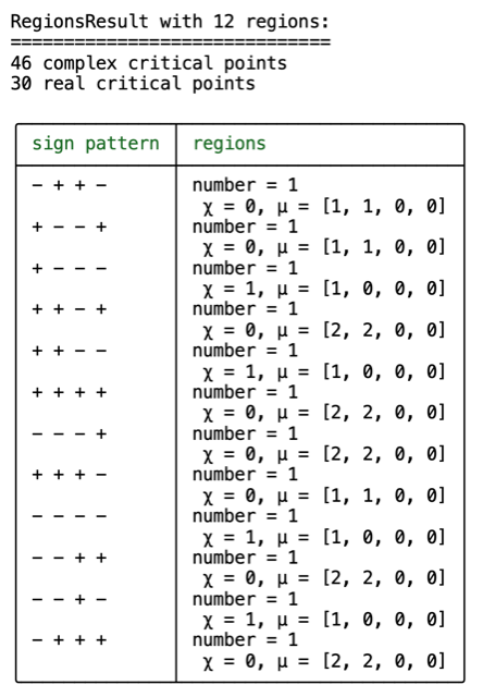
The output is shown in Figure 4. Eight of the sign patterns are realizable. The parameter plane is divided into regions. For instance, contributes two regions, one contractible and one with two holes (). The latter parametrizes polynomials with only two real roots. One sample point in that region is .
You are now invited to run the following code and to match its output with Figure 1:
A range of additional features is available in HypersurfaceRegions.jl. For instance, one finds the critical points in the -th region of the output by running the following command:
One can also locate the region to which a given point (e.g. the origin) belongs, as follows:
We next discuss a few implementation details. We use monodromy [9], implemented in HomotopyContinuation.jl [5], for computing the critical points of . The ODE solver from DifferentialEquations.jl [14] is used for the Morse flows (9) between critical points.
To find critical points, we solve the rational function equations in (4). These are equations in variables and parameters . For the monodromy, we need a start pair such that is a solution for with parameters . Since is linear in , we can use linear algebra to get such a start pair. Indeed, we can sample a random point and compute by solving linear equations. However, this works only if , and if has full rank. To avoid these issues, we use the following trick. If , we define new auxiliary parameters . Using monodromy, we solve the system , where and are random matrices. Afterwards, we track the homotopy from to using the solutions we have just computed. The parameter continuation theorem [15, 4] asserts that this approach works.
We modified the default options in HomotopyContinuation.jl for the monodromy loops. In HypersurfaceRegions.jl, a computation finishes if the last new monodromy loops have not provided any new solutions. The number is a conservative parameter here. Its purpose is to increase the probability of finding all critical points. The tolerance parameter for bounded regions, as described in the end of Section 3, is set to the default value .
5 Experiments
This final section is dedicated to systematic experiments with our software. We experimented by running HypersurfaceRegions.jl on random instances, drawn from two classes:
-
1.
arrangements defined by random polynomials;
-
2.
arrangements defined by random spectrahedra.
The first class is self-explanatory. To create (1), we choose at random from some probability distribution on the space of inhomogeneous polynomials of degree in variables.
The second class requires an explanation. We fix positive integers and , and we draw samples from the -dimensional space of symmetric matrices. We consider the arrangement defined by the principal minors of the matrix
| (11) |
The distinguished region where all principal minors are positive is the spectrahedron.
The stratification of symmetric matrices by signs of principal minors was studied by Boege, Selover and Zubkov in [3]. We explore random low-dimensional slices of the Boege-Selover-Zubkov stratification. How many regions get created, and what is their topology?
Example 13 ().
A prominent spectrahedron is the elliptope, which is given by
The minors of this matrix give the six facet equations of the -dimensional cube . Our arrangement lives in , and it consists of these six planes plus the cubic surface
| (12) |
For an illustration see Figure 5. Only four of the six facets are shown for better visibility.

We run HypersurfaceRegions.jl on this instance. The arrangement has regions. All have Euler characteristic . The six facet planes of the cube divide into regions. One is bounded (the cube itself) and are unbounded cones. The surface (12) divides the cube into regions, and it divides four of the cones into unbounded regions, for a total of regions. The projective arrangement has regions.
We now describe our experiments with arrangements of generic hypersurfaces. We run HypersurfaceRegions.jl on polynomials in variables of degree and , where the coefficients are drawn independently from the standard Gaussian. Each experiment is carried out times, where is inverse proportional to the running time for each instance.
Our findings are presented in Table 1 for and in Table 2 for . For each row we fix the parameters and . The time is the average running time per instance. This is measured in seconds. The fourth column concerns the total number of regions. We report the minimum number and the maximum number across all instances. The fifth column similarly reports the range for the number of realizable sign vectors . The sixth column gives the maximal number of regions per fixed sign pattern. And, finally, in the last column we report the minimum and maximum observed for the Euler characteristics of the regions.
| time | min-max #reg | min-max | max reg | min-max | ||
Let us discuss the first row in Table 1. The code runs seconds, and it identifies distinct regions in , where . The number of realizable sign patterns is at most . This is less than the number of all sign patterns. There were up to regions per sign pattern. The Euler characteristic of any region was between and .
| time | min-max #reg | min-max | max reg | min-max | ||
Table 2 presents analogous results for cubics in where . The second-last row concerns quintuples of cubics in . It takes less than six minutes to identify all regions, of which there are up to . We observed a narrow range of Euler characteristics.
Generic instances have no tangencies to the hyperplane at infinity. To experiment with that issue, we can try paraboloids in . Each paraboloid contributes one undecided region touching the hyperplane at infinity. Here is an instance of paraboloids for :
The output in Figure 6 consists of six regions, each with a unique sign pattern. Notice that the label “undecided” does not mean we claim this region touches the hyperplane at infinity. It means that our algorithm could not decide whether this region is bounded or unbounded.

We now turn to random spectrahedra. We sampled symmetric matrices where the entries are independent standard Gaussians. The principal minors of the matrix define an arrangement of hypersurfaces in the affine space . We ran HypersurfaceRegions.jl on this input. Our results are summarized in Table 3. For each row we fix the parameters and . The columns have the same meaning as before. For instance, the fifth column reports the range for the number of realizable sign vectors .
| time | min-max #reg | min-max | max reg | min-max | ||
We also performed computations for , but we do not report them because we ran into numerical issues. Frequently, the Hession of (6) at some critical point is almost singular.
References
- [1] J. Bezanson, A. Edelman, S. Karpinski and V. Shah: Julia: A fresh approach to numerical computing, SIAM Review 59 (2017) 65–98.
- [2] J. Bisgard: Mountain passes and saddle points, SIAM Review 57 (2015) 275–292.
- [3] T. Boege, J. Selover and M. Zubkov: Sign patterns of principal minors of real symmetric matrices, arXiv:2407.17826.
- [4] V. Borovik and P. Breiding: A short proof for the parameter continuation theorem, Journal of Symbolic Computation 127 (2025).
- [5] P. Breiding and S. Timme: HomotopyContinuation.jl: A package for homotopy continuation in Julia, Math. Software, ICMS 2018, Lecture Notes in Comp. Science, 10931, 458-465, 2018.
- [6] F. Catanese, S. Hoşten, A. Khetan and B. Sturmfels: The maximum likelihood degree, American J. Math. 128 (2006) 671–697.
- [7] D. Cohen, G. Denham, M. Falk and A. Varchenko: Critical points and resonance of hyperplane arrangements, Canadian Journal of Mathematics 63 (2011) 1038–1057.
- [8] J. Cummings, J. Hauenstein, H. Hong and C. Smyth: Smooth connectivity in real algebraic varieties, arXiv:2405.18578.
- [9] T. Duff, C. Hill, A. Jensen, K. Lee, A. Leykin and J. Sommars: Solving polynomial systems via homotopy continuation and monodromy, IMA J. Numerical Analysis 39 (2019) 1421–1446.
- [10] N. Early, A. Geiger, M. Panizzut, B. Sturmfels and C. Yun: Positive del Pezzo geometry, arXiv:2306.13604.
- [11] H. Hong, J. Rohal, M. Safey El Din and E. Schost: Connectivity in semi-algebraic sets: I, arXiv:2011.02162.
- [12] J. Moré and T. Munson: Computing mountain passes and transition states, Mathematical Programming 100 (2004) 151–182.
- [13] L. Nicolaescu: An Invitation to Morse Theory, Universitext, Springer, Berlin, 2011.
- [14] C. Rackauckas and Q. Nie: Differentialequations.jl – a performant and feature-rich ecosystem for solving differential equations in Julia, Journal of Open Research Software 5 (2017) 15.
- [15] A. Sommese and C. Wampler: The Numerical Solution of Systems of Polynomials Arising in Engineering and Science, World Scientific, 2005.
- [16] R. Stanley: An introduction to hyperplane arrangements, Geometric Combinatorics, American Mathematical Society, IAS/Park City Mathematics Series 13 (2007) 389–496.
- [17] B. Sturmfels and S. Telen: Likelihood equations and scattering amplitudes, Algebraic Statistics 12 (2021) 167–186.
Authors’ addresses:
Paul Breiding, Universität Osnabrück [email protected]
Bernd Sturmfels, MPI MiS Leipzig [email protected]
Kexin (Ada) Wang, Harvard University kexin[email protected]