Computationally efficient variational-like approximations of possibilistic inferential models111This is an extended version of the paper (Cella and Martin, 2024) presented at the 8th International Conference on Belief Functions, in Belfast, UK.
Abstract
Inferential models (IMs) offer provably reliable, data-driven, possibilistic statistical inference. But despite IMs’ theoretical and foundational advantages, efficient computation is often a challenge. This paper presents a simple and powerful numerical strategy for approximating the IM’s possibility contour, or at least its -cut for a specified . Our proposal starts with the specification a parametric family that, in a certain sense, approximately covers the credal set associated with the IM’s possibility measure. Then the parameters of that parametric family are tuned in such a way that the family’s credible set roughly matches the IM contour’s -cut. This is reminiscent of the variational approximations now widely used in Bayesian statistics, hence the name variational-like IM approximation.
Keywords and phrases: Bayesian; confidence regions; credal set; fiducial; Monte Carlo; stochastic approximation.
1 Introduction
For a long time, despite Bayesians’ foundational advantages, few statisticians were actually using Bayesian methods—the computational burden was simply too high. Things changed significantly when Monte Carlo methods brought Bayesian solutions within reach. Things changed again more recently with the advances in various approximate Bayesian computational methods, in particular, the variational approximations in Blei et al., (2017), Tran et al., (2021), and the references therein. The once clear lines between what was computationally feasible for Bayesians and for non-Bayesians have now been blurred, reinvigorating Bayesians’ efforts in modern applications. Dennis Lindley predicted that “[statisticians] will all be Bayesians in 2020” (Smith, 1995)—his prediction did not come true, but the Bayesian community is arguably stronger now than ever.
While Bayesian and frequentist are currently the two mainstream schools of thought in statistical inference, these are not the only perspectives. For example, Dempster–Shafer theory originated as an improvement to and generalization of both Bayesian inference and Fisher’s fiducial argument. Of particular interest to us here are the recent advances in inferential models (IMs, Martin and Liu, 2013; Martin and Liu, 2015b ; Martin, 2021a ; Martin, 2022b ), a framework that offers Bayesian-like, data-dependent, possibilistic quantification of uncertainty about unknowns but with built-in, frequentist-like reliability guarantees. IMs and other new/non-traditional frameworks are currently facing the same computational challenges that Bayesians faced years ago. That is, we know what we want to compute and why, but we are currently lacking the tools to do so efficiently. While traditional Monte Carlo methods are still useful (see Section 2), the imprecision that is key to the IM’s reliability guarantees implies that Monte Carlo methods alone are not enough. In contrast to Lindley’s prediction, for Efron’s speculation about fiducial and related methods—“Maybe Fisher’s biggest blunder will become a big hit in the 21st century!” (Efron, 1998)—to come true, imprecision-accommodating advances in Monte Carlo computations are imperative. The present paper’s contribution is in this direction.
We start with a relatively simple idea that leads to a general tool for computationally efficient and statistically reliable possibilistic inference. For reasons summarized in Section 2, our focus is on the possibility-theoretic brand of IMs, which are fully determined by the corresponding contour function or, equivalently, the contour function’s so-called -cuts. We leverage a well-known characterization of a possibility measure’s credal set as the collection of probability measures that assign probability at least to the aforementioned -cuts of the contour function. In the IM context, the -cuts are % confidence regions and, therefore, the contents of the IM’s credal set can be justifiably interpreted as “confidence distributions” (e.g., Xie and Singh, 2013; Schweder and Hjort, 2002). Specifically, the “most diffuse” element of the credal set, or “inner probabilistic approximation,” would assign probabilities as close to as possible to each -cut. If we could approximate this distinguished member of the IM’s credal set, via Monte Carlo or otherwise, then we would be well on our way to carrying out most—if not all—of the relevant IM computations. The challenge is that, except for very special classes of problems (Martin, 2023a ), this “inner probabilistic approximation” would be rather complex. We can, however, obtain a relatively simple approximation if we only require an accurate approximation of, say, a single -cut. Towards this, we propose to introduce a simple parametric family of probability distributions, e.g., Gaussian, on the parameter space, with parameters partially depending on data, and then choosing those unspecified features of the parameter in such a way that the distribution (approximately) assigns probability to a specified -cut, say, . This is akin to variational Bayes in the sense that we propose to approximate a complex probability distribution—in our case it is the “inner probabilistic approximation” of the IM’s possibility measure instead of a Bayesian posterior distribution—by an appropriately chosen member of a posited class of relatively simple probability distributions. The specific, technical details our proposal here are inspired by the recent work in Jiang et al., (2023) and the seemingly unrelated developments in Syring and Martin, (2019).
The remainder of the paper is organized as follows. After some background on possibilsitic IMs and their properties in Section 2, we present our basic but very general variational-like IM approximation in Section 3, which relies on a combination of Monte Carlo and stochastic approximation to tune the index of the posited parametric family of approximations. This is ideally suited for statistical inference problems involving low-dimensional parameters, and we offer a few such illustrations in Section 4. A more sophisticated version of the proposed variational-like approximation is presented in Section 5, which is more appropriate when the problem at hand is of higher dimension, but it is suited primarily for Gaussian approximation families—which is no practical restriction. With a more structured approximation, we can lower the computational cost by reducing the number of Monte Carlo evaluations of the IM contour. This is illustrated in several examples, including a relatively high-dimensional problem with lasso penalization and in problems involving nuisance parameters in parametric, nonparametric, and semiparametric models, respectively. The paper concludes in Section 7 with a concise summary and a discussion of some practically relevant extensions.
2 Background on possibilistic IMs
The first presentation of the IM framework (e.g., Martin and Liu, 2013; Martin and Liu, 2015b ) relied heavily on (nested) random sets and their corresponding belief functions. The more recent IM formulation in Martin, 2022b , building off of developments in Martin, (2015, 2018), defines the IM’s possibility contour using a probability-to-possibility transform applied to the relative likelihood. This small-but-important shift has principled motivations but we can only barely touch on this here. The present review focuses on the possibilistic IM formulation, its key properties, and the available computational strategies.
Consider a parametric statistical model indexed by a parameter space . Examples include , , with , and many others; see Section 4. Nonparametric problems—see Cella, (2024), Cella and Martin, (2022), and Martin, 2023b (, Sec. 5)—can also be handled, but we postpone discussion of this until Section 6. Suppose that the observable data consists of iid samples from the distribution , where is the unknown/uncertain “true value.” The model and observed data together determine a likelihood function and a corresponding relative likelihood function
Throughout we will implicitly assume that the denominator is finite, i.e., that the likelihood function is bounded for almost all .
The relative likelihood, , itself is a data-dependent possibility contour, i.e., it is a non-negative function such that for almost all . This contour, in turn, determines a possibility measure, or consonant plausibility function, that can be used for uncertainty quantification about , given , which has been extensively studied (e.g., Shafer, 1982; Wasserman, 1990; Denœux, 2006, 2014). Specifically, uncertainty quantification here would be based on the possibility assignments
where represents a hypothesis about . This purely likelihood-driven possibility measure has a number of desirable properties: for example, inference based on thresholding the possibility scores (with model-independent thresholds) satisfies the likelihood principle (e.g., Birnbaum, 1962; Basu, 1975), and it is asymptotically consistent (under standard regularity conditions) in the sense that it converges in -probability to a possibility measure concentrated on as . What the purely likelihood-based possibility measure above lacks, however, is a calibration property (relative to the posited model) that gives meaning or belief-forming inferential weight to the “possibility” it assigns to hypotheses about the unknown . More specifically, if we offer a possibility measure as our quantification of statistical uncertainty, then its corresponding credal set should contain probability distributions that are statistically meaningful. We are assuming vacuous prior information, so there are no meaningful or distinguished Bayesian posterior distributions. The only other natural property to enforce on the credal set’s elements is that they be “confidence distributions.” But, as in (5), this interpretation requires the -cuts of the relative likelihood, i.e., , to be % confidence sets for , which generally they are not. Therefore, the relative likelihood alone is not enough.
Fortunately, it is at least conceptually straightforward to achieve this calibration by applying what Martin, 2022a calls “validification”—a version of the probability-to-possibility transform (e.g., Dubois et al., 2004; Hose, 2022). In particular, for observed data , the possibilistic IM’s contour is defined as
| (1) |
and the possibility measure—or upper probability—is
A corresponding necessity measure, or lower probability, is defined via conjugacy as . This measure plays a crucial role in quantifying the support for hypotheses of interest (Cella and Martin, 2023); see Example 5.
An essential feature of this IM construction is its so-called validity property:
| (2) |
This has a number of important consequences. First, (2) is exactly the calibration property required to ensure a “confidence” connection that the relative likelihood on its own misses. In particular, (2) immediately implies that the set
| (3) |
indexed by , is a % frequentist confidence set in the sense that its coverage probability is at least :
Moreover, it readily follows that
| (4) |
In words, the IM is valid, or calibrated, if it assigns possibility to true hypotheses at rate as a function of data . This is precisely where the IM’s aforementioned “inferential weight” comes from: (4) implies that we do not expect small when is true, so we are inclined to doubt the truthfulness of those hypotheses for which is small. In addition, the above property ensures that the possibilistic IM is safe from false confidence (Balch et al., 2019; Martin, 2019, 2024), unlike all default-prior Bayes and fiducial solutions. An even stronger, uniform-in-hypotheses version of (4) holds, as shown/discussed in Cella and Martin, (2023):
The “for some with ” event can be seen as a union of every hypothesis that contains , which makes it a much broader event than that associated with any single fixed in (4). Consequently, regardless of the number of hypotheses evaluated or the manner in which they are selected—even if they are data-dependent—the probability that even a single suggestion from the IM is misleading remains controlled at the specified level. For further details about and discussion of the possibilistic IM’s properties, its connection to Bayesian/fiducial inference, etc, see Martin, 2022b ; Martin, 2023b ; Martin, 2023a .
In a Bayesian analysis, inference is based on summaries of the data-dependent posterior distribution, e.g., posterior probabilities of scientifically relevant hypotheses, expectations of loss/utility functions, etc. And all of these summaries boil down to integration involving the probability density function that determines the posterior. Virtually the same statement is true of the possibilistic IM: the lower–upper probability pairs for scientific relevant hypotheses, lower–upper expectations of loss/utility functions, etc. boil down to optimization involving the possibility contour . For example, if the focus is on a certain feature of , then the Bayesian can find the marginal posterior distribution for by integrating the posterior density for . Similarly, the corresponding marginal possibilistic IM has a contour that is obtained by optimizing :
Importantly, unlike with Bayesian integration, the IM’s optimization operation ensures that the validity property inherent in is transferred to , which implies that the IM’s marginal inference about is safe from false confidence.
The above-described operations applied to the IM’s contour function (1), to obtain upper probabilities or to eliminate nuisance parameters, are all special cases of Choquet integrals (e.g. Troffaes and de Cooman, 2014, App. C). These more general Choquet integrals can be statistically relevant in formal decision-making contexts (Martin, 2021b ), etc. For the sake of space, we will not dig into these details here, but the fact that there are non-trivial operations to be carried out even after the IM’s contour function has been obtained provides genuine, practical motivation for us to find the simplest and most efficient contour approximation as possible.
While the IM construction and properties are relatively simple, computation can be a challenge. The key observation is that we rarely have the sampling distribution of the relative likelihood , under , available in closed form to facilitate exact computation of for any . So, instead, the go-to strategy is to approximate that sampling distribution using Monte Carlo at each value of on a sufficiently fine grid (e.g., Martin, 2022b ; Hose et al., 2022). That is, the possibility contour is approximated as
where is the indicator function and consists of iid samples from for . The above computation is feasible at one or a few different values, but it is common that this needs to be carried out over a sufficiently fine grid covering the (relevant area) of the often multi-dimensional parameter space . For example, the confidence set in (3) requires that we can solve the equation , or at least find which ’s satisfy , and a naive approach is to compute the contour over a huge grid and then keep those that (approximately) solve the aforementioned equation. This amounts to lots of wasted computations. More generally, the relevant summaries of the IM output involve optimization of the contour, and carrying out this optimization numerically requires many contour function evaluations. Simple tweaks to this most-naive approach can be employed in certain cases, e.g., importance sampling, but these adjustments require problem-specific considerations and they cannot be expected to offer substantial improvements in computational efficiency. This is a serious bottleneck, so new and not-so-naive computational strategies are desperately needed.
3 Basic variational-like IMs
The Monte Carlo-based strategy reviewed above is not the only way to numerically approximate the possibilistic IM. Another option is an analytical “Gaussian” approximation (see below) based on the available large-sample theory (Martin and Williams, 2024). The goal here is to strike a balance between the (more-or-less) exact but expensive Monte Carlo-based approximation and the rough but cheap large-sample approximation. To strike this balance, we choose to focus on a specific feature of the possibilistic IM’s output, namely, the confidence sets in (3), and choose the approximation such that it at least matches the given confidence set exactly. Our specific proposal resembles the variational approximations that are now widely used in Bayesian analysis, where first a relatively simple family of candidate probability distributions is specified and then the approximation is obtained by finding the candidate that minimizes (an upper bound on) the distance/divergence from the exact posterior distribution. Our approach differs in the sense that we are aiming to approximate a possibility measure by (the probability-to-possibility transform applied to) an appropriately chosen probability distribution.
Following Destercke and Dubois, (2014), Couso et al., (2001), and others, the possibilistic IM’s credal set, , which is the set of precise probability distributions dominated by , has a remarkably simple and intuitive characterization:
| (5) |
(Where convenient, we will replace the subscript “” by a subscript “”—e.g., and instead of and —to simplify the notation in what follows.) That is, a data-dependent probability is consistent with if and only if, for each , it assigns at least mass to the IM’s confidence set in (3). Furthermore, the “best” inner probabilistic approximation of the possibilistic IM, if it exists, corresponds to a such that for all . For a certain special class of statistical models, Martin, 2023a showed that this best inner approximation corresponds to Fisher’s fiducial distribution and the default-prior Bayesian posterior distribution. Beyond this special class of models, however, it is not clear if a best inner approximation exists and, if so, how to find it. A less ambitious goal is to find, for a fixed choice of , a probability distribution such that
| (6) |
Our goal here is to develop a general strategy for finding, for a given , a probability distribution that (at least approximately) solves the equation in (6). Once identified, we can reconstruct relevant features of the possibilistic IM via (Bayesian-like) Monte Carlo sampling from this .
We propose to start with a parametric class of data-dependent probability distributions indexed by a generic space . An important example is the case where the ’s are Gaussian distributions with mean vector and/or covariance matrix depending on (data and) in some specified way. Specifically, since the possibilistic IM contour’s peak is at the maximum likelihood estimator , it makes sense to fix the mean vector of the Gaussian at ; for the covariance matrix, however, a natural choice would be , where is the observed Fisher information matrix depending on data and on the posited statistical model. This Gaussian family is a very reasonable default choice of given that with is asymptotically the best inner probabilistic approximation to ; see Martin and Williams, (2024). So, our proposal is to insert some additional flexibility in the Gaussian approximation by allowing the spread to expand or contract depending on whether or . While a Gaussian-based approximation is natural, choosing to be a Gaussian family is not the only option for ; see Example 4 below. Indeed, if the parameter space has structure that is not present in the usual Euclidean space where the Gaussian is supported, e.g., if is the probability simplex, then choosing to respect that structure makes perfect sense.
The one high-level condition imposed on is that it be sufficiently flexible, i.e., as varies, the -probability of the possibilistic IM’s -cut takes values smaller and larger than the target level . This clearly holds for the Gaussian approximation described above, since controls the spread of to the extent that the aforementioned -probability can be made arbitrarily small or large by taking sufficiently small or large, respectively. This mild condition can also be readily verified for virtually any other (reasonable) approximation family .
Given such a suitable choice of approximation family , indexed by a parameter , our proposed procedure is as follows. Define an objective function
| (7) |
so that solving (6) boils down to finding a root of . If the probability on the right-hand side of (7) could be evaluated in closed-form, then one could apply any of the standard root-finding algorithms to solve this, e.g., Newton–Raphson. However, this -probability typically cannot be evaluated in closed-form so, instead, can be approximated via Monte Carlo with defined as
| (8) |
where . Presumably, the aforementioned samples are cheap for every because the family has been specified by the user. But only having an unbiased estimator of the objective function requires some adjustments to the numerical routine. In particular, rather than a Newton–Raphson routine that assumes the function values are noiseless, we must use a stochastic approximation algorithm (e.g., Syring and Martin, 2021, 2019; Martin and Ghosh, 2008; Kushner and Yin, 2003; Robbins and Monro, 1951) that is adapted to noisy function evaluations of . The basic Robbins–Monro algorithm seeks the root of (7) through the updates
where “” depends on whether is decreasing or increasing, is an initial guess, and is a deterministic step size sequence that satisfies
Pseudocode for our proposed approximation is given in Algorithm 1. To summarize, we are proposing a simple data-dependent probability distribution for whose probability-to-possibility contour closely matches the IM’s contour at least at the specified threshold . More specifically, a reasonable choice of probability distribution is a Gaussian, and the approach presented in Algorithm 1 scales the covariance matrix so that its corresponding contour function accurately approximates the IM’s contour at threshold .
It is well-known that, under certain mild conditions, the sequence as defined above converges in probability to the root of in (7). If is the value returned when the algorithm reaches practical convergence, e.g., when or the change is smaller than some specified threshold, then we set . This distribution should be at least a decent approximation of the IM possibility measure’s inner approximation, i.e., the “most diffuse” member of . Consequently, the probability-to-possibility transform in (1) applied to should be a decent approximation of the exact possibilistic IM contour , at least in terms of their upper -cuts. The illustrations presented in Section 4 below show that our proposed approximation is much better than “decent” in cases where we can visually compare with the exact IM contour.
As emphasized above, a suitable choice of depends on context. An important consideration in this choice is the ability to perform exact computations of the approximate contour determined by the inner approximation . This is the case for the aforementioned normal variational family , with mean and covariance , as
| (9) |
where is the distribution function. This closed-form expression makes summaries of the contour, which are approximations of certain features (e.g., Choquet integrals) of the possibilistic IM , relatively easy to obtain numerically.
4 Numerical illustrations
Our first goal here is to provide a proof-of-concept for the proposed approximation. Towards this, we present a few low-dimensional illustrations where we can visualize both the exact and approximation IM contours and directly assess the quality of the approximation. In all but Example 4 below, we use the normal variational family with mean and covariance as described above, with to be determined. All of the examples display the variational-like IM approximation based on , Monte Carlo samples, step sizes , and convergence threshold .
Example 1.
Suppose the data is with probability mass function . The exact IM possibility contour based on is
| (10) |
where is the binomial relative likelihood of for successes:
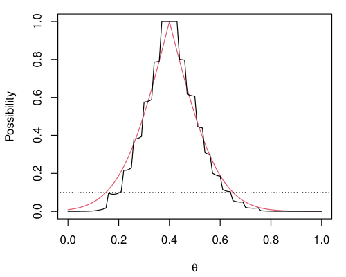
The right-hand side of (10) can be evaluated numerically without Monte Carlo. This and the contour corresponding to the proposed Gaussian-based variational approximation are shown in Figure 1(a) for and successes. Note that the two contours closely agree, especially at the level specifically targeted.
Example 2.
Suppose consists of iid bivariate normal pairs with zero means and unit variances, with common density function
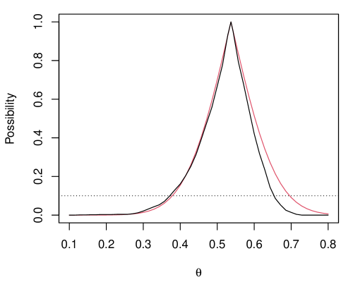
Inference on the unknown correlation is a surprisingly challenging problem (e.g., Basu, 1964; Reid, 2003; Martin and Liu, 2015a ). Indeed, despite being a scalar exponential family model, it does not have a one-dimensional sufficient statistic and, moreover, there are a variety of different ancillary statistics on which to condition, leading to different solutions. From a computational perspective, it is worth noting that the maximum likelihood estimation is not available in closed-form—in particular, it is not the sample correlation coefficient. That this optimization is non-trivial adds to the burden of a naive Monte Carlo IM construction. Figure 1(b) shows the exact IM contour, based on a naive Monte Carlo implementation of (1), which is rather expensive, and the approximation for simulated data of size with true correlation 0.5. The exact contour has some asymmetry that the normal approximation cannot perfectly accommodate, but it makes up for this imperfection with a slightly wider upper 0.1-level set.
Example 3.
The data presented in Table 8.4 of Ghosh et al., (2006) concerns the relationship between exposure to chloracetic acid and mouse mortality. A simple logistic regression model is to be fit in order to relate the binary death indicator () with the levels of exposure () to chloracetic acid for the dataset’s mice. That is, consists of independent pairs and a conditionally Bernoulli model for , given , with mass function
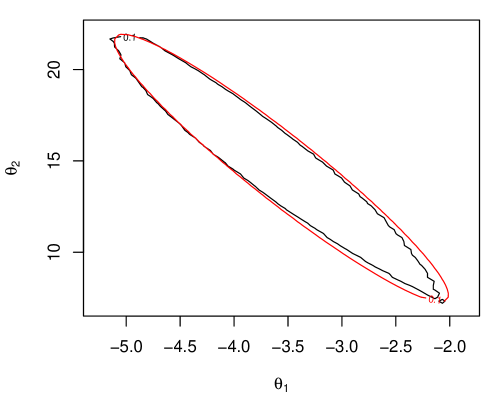
where is the logistic distribution function. The corresponding likelihood cannot be maximized in closed-form, but doing so numerically is routine. The maximum likelihood estimator and the corresponding observed information matrix lead to the asymptotically valid inference reported by standard statistical software packages. For exact inference, however, the computational burden is heavier: evaluating the validified relative likelihood over a sufficiently fine grid of values is rather expensive. Figure 1(c) presents the -level set of the exact IM possibility contour for the regression coefficients, based on a naive Monte Carlo implementation of (1), alongside the proposed variational approximation. The latter’s computational cost is a small fraction of the former’s, and yet the two contours line up almost perfectly.
Example 4.
Consider iid data points sampled from with unknown probabilities belong the probability simplex in . The frequency table, , with being the frequency of category in the sample of size , is a sufficient statistic, having a multinomial distribution with parameters ; the probability mass function is
Here we use a Dirichlet variational family , parametrized in terms of the mean vector and precision , with density function
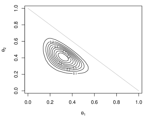
where, naturally, we take the mean to be the maximum likelihood estimator, , and the precision to be , where is to be determined. Of course, a Gaussian variational approximation could also be used here, but our use of the Dirichlet approximation aims to highlight our proposal’s flexibility. Figure 1(d) shows the approximate IM contour based on and counts . The exact IM contour is virtually impossible to evaluate, because naive Monte Carlo is slow, the contours are noisy when based on Monte Carlo sample sizes that are too small, and the discrete nature of the data gives it the unusual shape akin to the binomial plot in Figure 1(a). Here, however, we get a smooth contour approximation in a matter of seconds.
Our second goal in this section is to provide a more in-depth illustration of the kind of analysis that can be carried out with the proposed variational-like approximate IM. We do this in the context of regression modeling for count data.
Example 5.
Poisson log-linear models are widely used to analyze the relationship between a count-based discrete response variable and a set of fixed explanatory variables; even if the explanatory variables are not fixed by design, it is rare that their distribution would depend on any of the relevant parameters, so they are ancillary statistics and it is customary to condition on their observed values. Let represent the response variable, and denote the explanatory variables for the observation in a sample, . The Poisson log-linear model assumes that , where
The goal is to quantify uncertainty about the regression coefficients . Here, we will achieve this through the IMs framework.
Consider the data presented in Table 3.2 of Agresti, (2007), obtained from a study of the nesting habits of horseshoe crabs. In this study, each of the female horseshoe crabs had a male attached to her nest, and the goal was to explore factors influencing whether additional males, referred to as satellites, were present nearby. The response variable is the number of satellites observed for each female crab. Here, we focus on evaluating two explanatory variables related to the female crab’s size that may influence this response: , weight (kg), and , shell width (cm).
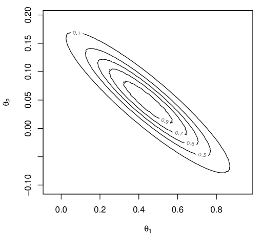
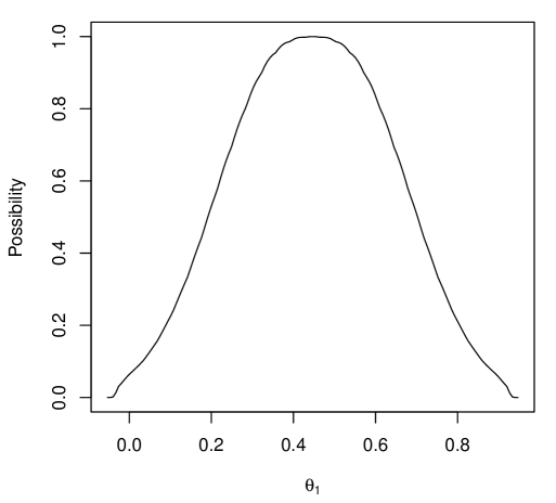
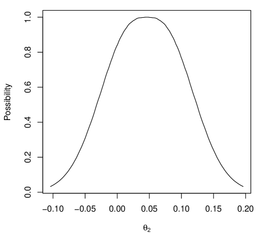
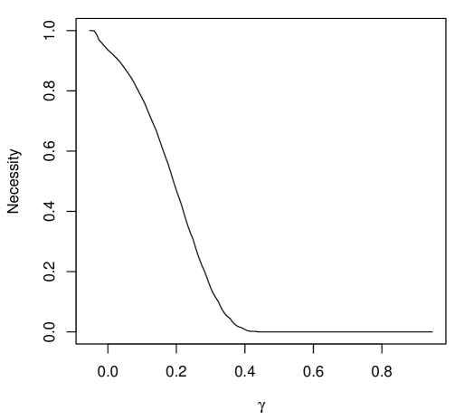
A variational approximation of the IMs contour was obtained from (9), with estimated using Monte Carlo samples, step sizes , and convergence threshold . Perhaps the first question to consider is whether at least one of or has an influence on . To address this, a marginal IM for is constructed, as shown in Figure 2(a). Notably, the hypothesis “” has an upper probability close to zero, providing strong evidence that at least one of or differs from zero. To evaluate the impact of and individually, the respective marginal IMs for and are shown in Figure 2(b,c). While there is strong evidence supporting “,” the hypothesis that “” is highly plausible. Finally, given the apparent evidence for “,” one might ask which hypotheses of the form “,” for , are well supported. This question can be addressed using the marginal necessity measures for , as shown in Figure 2(d). We can see that “” is well supported, indicating that an additional kilogram increases the average number of satellites per female crab by approximately . Importantly, the IM’s uniform validity insures that the probability that even one of the suggestions above is misleading is controllably small.
5 Beyond basic variational-like IMs
Various tweaks to the basic procedure described in Section 3 might be considered in order applications to speed up computations. If there is a computational bottleneck remaining in the proposal from Section 3, then it would have to be that the IM’s possibility contour must be evaluated at -many points in each iteration of the stochastic approximation. While this is not impractically expensive in some applications, including those presented above, it could be more of a burden in other applications. A related challenge is that a scalar index on the variational family, as we have focused on exclusively so far, may not be sufficiently flexible. Increasing the flexibility by considering higher-dimensional would likewise increase the computational burden, so care is needed. Here we aim to address both of the aforementioned challenges.
The particular modification that we consider here is best suited for cases where the variational family satisfies the following property: for each , the % credible set corresponding to can be expressed (or at least neatly summarized) in closed-form. The idea to be presented here is more general, but, to keep the details as simple and concrete as possible, we will focus our presentation on the case of a Gaussian variational family. Then the credible sets are ellipsoids in -dimensional space.
As a generalization of the scalar--indexed Gaussian family introduced in Section 3, let be a -vector index and take to be the -dimensional Gaussian family with mean vector , the maximum likelihood estimator, and covariance matrix defined as follows: take the eigen-decomposition of the observed Fisher information matrix as , and then set
That is, the components of act as multipliers on the singular values of . This indeed generalizes our previously-considered Gaussian approximation family since, if is a scalar, then we recover the previous covariance matrix: . Let denote the % credible set corresponding to the distribution . In the present -dimensional Gaussian case, this is an ellipsoid in , i.e.,
where is the quantile of the distribution. Then we know that assigns at least probability to the IM’s confidence set if
or, equivalently, if
For the Gaussian family of approximations we are considering here, the mode of , the maximum likelihood estimator, is in the interior of each credible set, so the behavior of outside is determined by its behavior on the boundary. Moreover, since equality in the above display implies a near-perfect match between the IM’s confidence sets and the posited Gaussian credible sets, a reasonable goal is to find a root to the function
where denotes the boundary of a set . In designing an iterative algorithm that makes steps towards this root, it is desirable to allow for steps of different magnitudes depending on the direction, and this requires care. For our present Gaussian approximation family, a natural—albeit minimal—representation of the boundary of the credible region is given by the collection of vectors
| (11) |
where is the eigenvalue–eigenvector pair corresponding to the largest eigenvalue. Then define the vector-valued function with components
| (12) |
At least intuitively, being less than or greater than 0 determines if the credible set is too large or too small, respectively in the -direction. From here, we can apply the same stochastic approximation procedure to determine a sequence , this time of -vectors, i.e.,
that converges to the root of which we expect to be close to the root of . The details of this new but familiar strategy are presented in Algorithm 2. The chief advantage of this new strategy compared to that summarized in Algorithm 1 is computational savings: each iteration of stochastic approximation in Algorithm 2 only requires (Monte Carlo) evaluation of the IM contour at many points, which would typically be far fewer than then number of Monte Carlo samples in Algorithm 1 needed to get a good approximation of .
We will illustrate this new version of the Gaussian variational family and approximation algorithm with two examples. The first is in the relatively simple two-parameter gamma model; the second is a relatively high-dimensional model involving a penalty, intended to serve a gateway into IM solutions to high-dimensional problems.
Example 6.
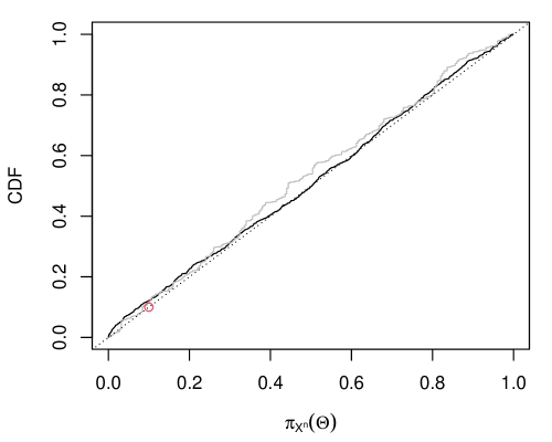
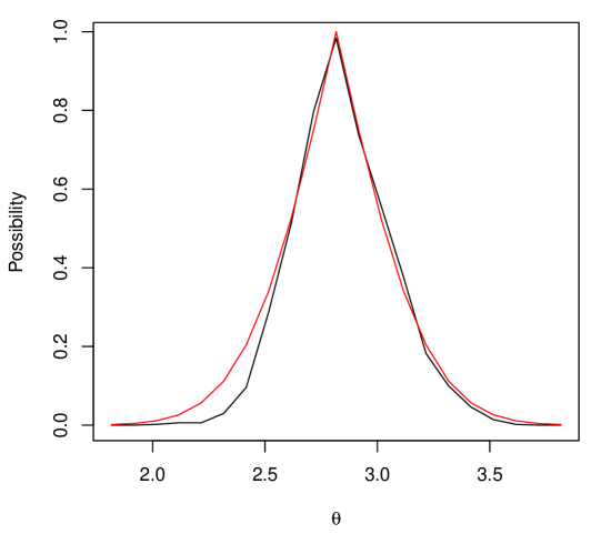
Suppose consists of an iid sample of size from a gamma distribution with shape parameter and scale parameter . We simulated data of size , with and , and we plot the approximate IM contour for in Figure 3(a). This contour is constructed by first building a Gaussian approximation of the contour for and then mapping the approximation back to the space. The parameters’ non-negativity constraints are gone when mapped to the log-scale, which improves the quality of the Gaussian approximation; the approximation is worse when applied directly on the space. For comparison, the contour of the relative likelihood is also shown, and its similarity to that of the Gaussian contour implies that the latter is a good approximation to the exact IM contour, which is rather expensive to compute. Indeed, Example 1 in Martin, (2018) considers exactly the same simulation setting and he also obtains a banana-shaped contour similar to the one in Figure 3(a).
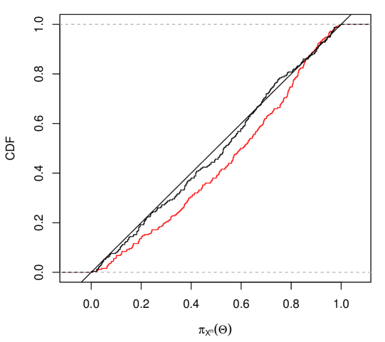
We also repeated the above example 1000 times and Figure 3(b) shows the distribution function of the random variable , based on both the exact contour and the Gaussian approximation. That with the exact contour is the distribution function (modulo Monte Carlo sampling variation) and that based on the Gaussian approximation is empirically indistinguishable from across the full range.

Example 7.
This simplest and most canonical high-dimensional inference example is the many-normal-means problem, which goes back to classical papers such as Stein, (1956), James and Stein, (1961), Brown, (1971), and others. The model assumes that the data consists of independent—but not iid—observations, with , where is assumed to be known but the vector is unknown and to be inferred. Roughly, the message in the references above is that the best unbiased estimator , also the maximum likelihood estimator, is inadmissible (under squared error loss). This result sparked research efforts on penalized estimation, including the now-famous lasso (e.g., Tibshirani, 1996, 2011). Following along these lines, and in the spirit of the examples in Section 6 above, we propose here to work with a relative penalized likelihood
where
is the penalized likelihood function, with and the - and -norms, respectively, and a tuning parameter to be discussed below. For this relatively simple high-dimensional model, the solution to the optimization problem in the denominator above, which is the lasso estimator, can be solved in closed-form: if the vector
is the solution, then its entries are given by
That is, the lasso penalization shrinks the maximum likelihood estimator of closer to 0 and, in fact, if the magnitude of is less than the specified , then the estimator is exactly 0. Of course, the choice of is critical, and here we will take it to be . In any case, we can construct a possibilistic IM contour as
Even though the relative penalized likelihood is available in closed-form, Monte Carlo methods are needed to evaluate this contour. And when the dimension is even moderately large, carrying out these computations on a grid in -dimensional space that is sufficiently fine to obtain, say, confidence sets for is practically impossible. But the variational approximation described above offers a computationally more efficient alternative to naive Monte Carlo that can handle moderate to large .
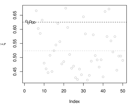
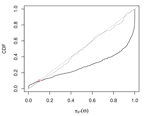
Here we follow the strategy suggested above, i.e., with a Gaussian approximation having mean equal to the lasso or maximum penalized likelihood estimator and covariance matrix indexed by the -vector ; in this case, the initial is taken to be the no-penalty information matrix , which is proportional to the identity matrix. The intuition here is that the coordinate-specific adjustment factors, , will allow the Gaussian approximation to adapt in some way to sparsity in the true signal . For our illustration, we consider and a true whose first five entries are equal to 5 and last 45 entries equal to 0, i.e., only 10% of the coordinates of contain a signal, the remaining 90% is just noise. We also fixed for the approximation. For a single data set, Figure 4(a) displays the estimates obtained at convergence of the proposed stochastic approximation updates. The points in black correspond to signals (non-zero true means) and the points in gray correspond to noise. The key observation is that values corresponding to signal tend to be larger than those corresponding to noise; there is virtually no variability in the signal cases, but substantial variability in the noise cases. That the values tend to be smaller in the noise case is expected, since much less spread in the IM’s possibility contour is needed around those means that are clearly 0. We repeated the above simulation 1000 times and plotted the distribution function of the exact (using naive Monte Carlo) and approximate (using the Gaussian variational family) IM contour at the true . Again, the exact contour at is distributed, and the results in Figure 4(b). The Gaussian approximation is only designed to be calibrated at level , which is clearly achieves; it is a bit too agressive at lower levels and conservative at the higher levels. Further investigation into this proposal in high-dimensional problems will be reported elsewhere.
6 Nuisance parameter problems
6.1 Parametric
The perspective taken above was that there is an unknown model parameter and the primary goal is to quantify uncertainty about in its entirety given the observed data from the model. Of course, quantification of uncertainty about implies quantification of uncertainty about any feature as described in Section 2 above. If, however, the sole objective is quantifying uncertainty about a particular , then it is natural to ask if we can do better than first quantifying uncertainty about the full and then deriving the corresponding results for . There are opportunities for efficiency gain, but this requires eliminating the nuisance parameters, i.e., those aspects of that are, in some sense, complementary or orthogonal to . One fairly general strategy for eliminating nuisance parameters is profiling (e.g., Martin, 2023b ; Severini and Wong, 1992; Sprott, 2000), described below.
It is perhaps no surprise that, while use of the relative likelihood in the IM construction presented in Section 2 is very natural and, in some sense, “optimal,” it is not the only option. For cases involving nuisance parameters, one strategy is to replace the relative likelihood in (1) with a surrogate, namely, the relative profile likelihood
| (13) |
Note that this is not based on a genuine likelihood function, i.e., there is no statistical model for , depending solely on the unknown parameter , for which is the corresponding likelihood function. Despite not being a genuine likelihood, the profile likelihood typically behaves very much like the usual likelihood asymptotically and, therefore, “may be used to a considerable extent as a full likelihood” (Murphy and van der Vaart, 2000, p. 449). In our present case, if we proceed with the relative profile likelihood in place of the relative likelihood in (1), then the marginal possibilistic IM has contour function
The advantage of this construction is that it tends to be more efficient than the naive elimination of nuisance parameters presented in Section 2; see, e.g., Martin and Williams, (2024). The outer supremum above is the result of not being the full parameter of the posited model; see Martin, 2023b (, Sec. 3.2) for more details. It is often the case that the probability on the right-hand side above is approximately constant in with , but one cannot count on this—the supremum needs to be evaluated, unfortunately, in order to ensure the IM’s strong validity properties hold marginally.
For concreteness, we will focus on a deceptively-challenging problem, namely, efficient inference on the mean of a gamma distribution. Roughly, the gamma mean is a highly non-linear function of the shape and scale parameters, which makes the classical, first-order asymptotic approximations of the sampling distribution of the maximum likelihood estimator rather poor in finite samples. For this reason, the gamma mean problem has received considerable attention, with focus on deriving asymptotic approximations with higher-order accuracy; we refer the reader to Fraser et al., (1997) for further details. Martin and Liu, 2015c presented an exact IM solution to the gamma mean problem and, more recently, a profile-based possibilistic IM solution was presented in Martin, 2023b (, Example 6) and shown to be superior to various existing methods. Here our focus is demonstrating the quality of the variational approximation in this new context.
Example 8.
Let the gamma model be indexed by , where and represent the (positive) shape and scale parameters, respectively. There are no closed-form expressions for the maximum likelihood estimators, and , in the gamma model, but one can readily maximize the likelihood numerically to find them; one can also obtain the observed Fisher information matrix , numerically or analytically. For the profile likelihood, it may help to reparametrize the model in terms of the mean parameter and the shape parameter . Write the density in this new parametrization as
In this form, the likelihood based on data could be maximized numerically over for any fixed , thus yielding the (relative) profile likelihood.
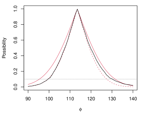
Fraser et al., (1997) presented an example where mice were exposed to 240 rads of gamma radiation and their survival times recorded. A plot of the exact profiling-based marginal possibilistic IM contour is shown (black line) in Figure 5. This is relatively expensive to compute since, at each point on the grid, our Monte Carlo approximation needs to be optimized over different values. For comparison, we consider a Gaussian possibility contour with mean and variance , where and the gradient is . Figure 5 shows the Gaussian approximation with as discussed in Martin and Williams, (2024) and with as identified based on our variational approximation from Section 5. This approximation takes only a fraction of a second to obtain, and we find that, as intended, it closely matches the exact contour at the target level on the right (heavy) side and is a bit conservative on the left (thin) side. Clearly the basic large-sample Gaussian approximation is too narrow in the right tail, confirming the claim above that the first-order asymptotic theory provides relatively poor approximations for smaller sample sizes. Our variational approximation, on the other hand, appropriately adjusts to match the exact contour in certain places while being a bit cautious or conservative in others.
6.2 Nonparametric
A nonparametric problem is one in which the underlying distribution is not assumed to have a particular form indexed by a finite-dimensional parameter. In some applications, it is itself (or, e.g., its density function) that is the quantity of interest and, in other case, there is some (finite-dimensional) feature or functional of that is to be inferred. Our focus here is on the latter case, so it also fits the general mold of a problem involving nuisance parameters, since all of what is left of once has been accounted for would be considered “nuisance” and to-be-eliminated.
At least in principle, one can approach this problem in a manner similar to that in the parametric case above, i.e., via profiling out those nuisance parts of . Recall that the goal of profiling is to reduce the dimension, so that the compatibility of data with candidate values of the quantity of interest could be directly assessed. Since it is typically the case that the quantity of interest has some real-world interpretation, there is an opportunity to leverage that interpretation for the aforementioned compatibility assessment without the need of profiling. This is the approach taken in Cella and Martin, (2022), building on the classical work in M-estimation (e.g., Huber, 1981; Stefanski and Boos, 2002) and less-classical work on Gibbs posteriors (e.g., Martin and Syring, 2022; Grünwald and Mehta, 2020; Bissiri et al., 2016; Zhang, 2006), which we summarize briefly below.
Let data consist of independent and identically distributed components with , where nothing is known or assumed about . In this more general case, the unknown quantity of interest is a functional of the underlying distribution. Examples include quantiles and moments of . Suppose can be expressed as the minimizer of a risk or expected loss function. That is, assume that there exists a loss function such that
where is the risk or expected loss function. An empirical version of the risk function replaces expectation with respect to by averaging over observations:
Then the empirical risk minimizer, , is the natural estimator of the risk minimizer . From here, we can mimic the relative likelihood construction with an empirical-risk version
Clearly, values of such that is close to 1 are more compatible with data than values of such that it is close to 0. Note that no profiling over the infinite-dimensional nuisance parameters is required in evaluating .
The same validification step can be taken to construct a possibilistic IM:
| (14) |
The outer supremum, analogous to that in (13), maximizes over all those probability distributions such that the relevant feature of takes value . This supremum appears because the distribution of obviously depends on the underlying , but this is unknown. This puts direct evaluation of the IM contour based on naive Monte Carlo out of reach. Fortunately, validity only requires that certain calibration holds for the one true , which provides a shortcut. Cella and Martin, (2022) proposed to replace “iid sampling from for all -compatible ” with iid sampling from the empirical distribution, which is a good estimator of the one true . This amounts to using the bootstrap (e.g., Efron, 1979; Efron and Tibshirani, 1993; Davison and Hinkley, 1997) to approximate the above contour, and Cella and Martin prove that the corresponding IM is asymptotically valid. Here, we will demonstrate that the proposed variational-like IMs can provide a good approximation for this bootstrap-based contour.
Example 9.
Suppose interest in the -th quantile of a distribution , i.e., the exact point such that , for . The key component in the nonparametric IM construction above is selecting an appropriate loss function. For quantile estimation, it is well-known that the loss function is given by
Figure 6(a) shows the bootstrap approximation of the IM contour in (14), computed using 500 bootstrap samples, for a dataset of size and . We chose to work with the normal family for the variational approximation, due to the well known asymptotic normality of the empirical risk minimizer (sample quantile) :
where represents the common density function associated with the underlying true distribution . More specifically, our chosen Gaussian variational family has mean and variance
where denotes a kernel density estimate of based on the observed data. The same settings as in Section 4 were applied, with estimated using Monte Carlo samples, step sizes , and convergence threshold Note how the variational approximation is perfect except for small levels of on the left side, where it is a bit conservative.
To verify that the variational approach provides approximate validity in nonparametric settings, a simulation study was performed by repeating the above scenario 250 times. For each dataset, the approximated contour was evaluated at , which corresponds approximately to the first quartile when follows a distribution. The empirical distribution of this contour is shown in Figure 6(b), demonstrating that approximate validity is indeed achieved.
6.3 Semiparametric
A middle-ground between the parametric and nonparametric case described in the previous two subsections is what are called semiparametric problems, i.e., those with parametric and nonparametric parts. Perhaps the simplest example is a linear regression model with an unspecified error distribution: the linear mean function is the parametric part and the error distribution is the nonparametric part. Below we will focus on a censored-data with a semiparametric model but, of course, other examples are possible; see, e.g., Bickel et al., (1998), Tsiatis, (2006), and Kosorok, (2008) for more details.
The same profiling strategy described in Section 6.1 above can be carried out for semiparametric models too; Murphy and van der Vaart, (2000) is an important reference. For concreteness, we will consider a common situation involving censored data. That is, suppose we are measuring, say, the concentration of a particular chemical in the soil, but our measurement instrument has a lower detectability limit, i.e., concentrations below this limit are undetectable. In such cases, the concentrations are (left) censored. We might have a parametric model in mind for the measured concentrations, but the censoring corrupts the data and ultimately changes that model. Let denote the actual chemical concentration at site , which we may or may not observe; the ’s are assigned a statistical model , and the true-but-unknown value of the posited model parameter is to be inferred. Let denote the censoring level, which we will assume—without loss of generality—to be subject to sampling variability, i.e., the ’s are random variables. Then the observed data consists of iid pairs , where
| (15) |
The goal is to infer the unknown in the model for the concentrations, but now the measurements are corrupted by censoring. The augmented model for the corrupted data has likelihood function given by
depending on both the generic value of the true unknown model parameter for the concentrations and on the generic value of the true unknown censoring level distribution . In the above expression, and are density functions for the censoring and concentration distributions, and and are the corresponding cumulative distribution functions. Now it should be clear why this is a semiparametric model: in addition to the obvious parametric model, there is the nonparametric model for the censoring levels.
A distinguishable feature of this semiparametric model is that the likelihood function is “separable,” i.e., it is a product of terms involving and terms involving . Consequently, if we were to optimize over and then form the relative profile likelihood ratio, then the part involving the optimization over cancels out. This implies that we can simply ignore the part with and work with the relative profile likelihood of the form
where is the maximum likelihood estimator of . The distribution of the relative profile likelihood still depends on the nuisance parameter , so when we define the possibilistic IM contour by validifying the relative profile likelihood, we get
Similar to the strategy described above (from Cella and Martin, 2022) for the nonparametric problem, Cahoon and Martin, (2021) proposed a novel strategy wherein a variation on the Kaplan–Meier estimator (e.g., Kaplan and Meier, 1958; Klein and Moeschberger, 2003) is used to obtain a , and then the contour above is approximated by
| (16) |
Evaluation of the right-hand side via Monte Carlo boils down to sampling censoring levels from , sampling concentration levels from , and then constructing new data sets according to (15). While this procedure is conceptually relatively simple, naive implementation over a sufficiently fine grid of values is rather expensive. Fortunately, our proposed variational-like approximation from Section 5 can be readily applied, quickly producing an approximate contour in closed-form.
Example 10.
For illustration, we use data on Atrazine concentration collected from a well in Nebraska. The data consists of observations subjected to random left-censoring as described above. This is a rather extreme case where nearly half (11) of the 24 observations are censored, but previous studies indicate that a log-normal model for the Atrazine concentrations is appropriate (Helsel, 2005). The log-normal distribution is often used to model left-censored data in environmental science applications (Krishnamoorthy and Xu, 2011, e.g.,). The log-normal model density is
where represent the mean and variance parameters for . Again, log-normal is only the model for the observed concentrations—no model is assumed for the censored observations. Figure 7(a) displays the nonparametric estimator of the censored data distribution obtained by applying the Kaplan–Meier estimator with the censoring labels swapped: . This is then used to define what we are referring to here as the “exact” IM contour via (16), and then the corresponding Gaussian variational approximation—applied to first and then mapped back to —is shown in Figure 7(b). This plot is very similar to that shown in Cahoon and Martin, (2021, Fig. 10) based on naive Monte Carlo, but far less expensive computationally.


7 Conclusion
In a similar spirit to the variational approximations that are now widely used in Bayesian statistics, and building on recent ideas presented in Jiang et al., (2023), we develop here a strategy to approximate the possibilistic IM’s contour function—or at least its -cuts/level sets for specified —using ordinary Monte Carlo sampling and stochastic approximation. A potpourri of applications is presented, from simple textbook problems to (parametric, nonparametric, and semiparametric) problems involving nuisance parameters, and even one of relatively high dimension, to highlight the flexibility, accuracy, and overall applicability of our proposal.
A number of important and practically relevant extensions to the proposed method can and will be explored. Here we will mention two such extensions. First, recent efforts (e.g., Martin, 2022b ) have focused on incorporating incomplete or partial prior information into the possibilistic IM; something along these lines is sure to be necessary as we scale up to problems of higher dimension. The only downside to the incorporation of partial prior information is that the evaluation of the IM contour is often even more complicated than in the vacuous-prior case considered here. Thanks to the added complexity, efficient numerical approximations are even more important in these partial-prior formulations and, fortunately, we expect that the proposal here will carry over more-or-less directly. Second, there is an obvious question of whether the -specific approximations developed here can, somehow, be stitched together in order to obtain an approximation that is (mostly) insensitive to the specification of any particular value. Inspired by the recent developments in Jiang et al., (2023), we believe that the answer to this question is Yes, and these important details will be reported elsewhere.
References
- Agresti, (2007) Agresti, A. (2007). An Introduction Categorical Data Analysis. John Wiley & Sons, 2nd edition.
- Balch et al., (2019) Balch, M. S., Martin, R., and Ferson, S. (2019). Satellite conjunction analysis and the false confidence theorem. Proc. Royal Soc. A, 475(2227):2018.0565.
- Basu, (1964) Basu, D. (1964). Recovery of ancillary information. Sankhyā Ser. A, 26:3–16.
- Basu, (1975) Basu, D. (1975). Statistical information and likelihood. Sankhyā Ser. A, 37(1):1–71. Discussion and correspondance between Barnard and Basu.
- Bickel et al., (1998) Bickel, P. J., Klaassen, C. A. J., Ritov, Y., and Wellner, J. A. (1998). Efficient and Adaptive Estimation for Semiparametric Models. Springer-Verlag, New York.
- Birnbaum, (1962) Birnbaum, A. (1962). On the foundations of statistical inference. J. Amer. Statist. Assoc., 57:269–326.
- Bissiri et al., (2016) Bissiri, P. G., Holmes, C. C., and Walker, S. G. (2016). A general framework for updating belief distributions. J. R. Stat. Soc. Ser. B. Stat. Methodol., 78(5):1103–1130.
- Blei et al., (2017) Blei, D. M., Kucukelbir, A., and McAuliffe, J. D. (2017). Variational inference: a review for statisticians. J. Amer. Statist. Assoc., 112(518):859–877.
- Brown, (1971) Brown, L. D. (1971). Admissible estimators, recurrent diffusions, and insoluble boundary value problems. Ann. Math. Statist., 42:855–903.
- Cahoon and Martin, (2021) Cahoon, J. and Martin, R. (2021). Generalized inferential models for censored data. Internat. J. Approx. Reason., 137:51–66.
- Cella, (2024) Cella, L. (2024). Distribution-free inferential models: Achieving finite-sample valid probabilistic inference, with emphasis on quantile regression. International Journal of Approximate Reasoning, 170:109211.
- Cella and Martin, (2022) Cella, L. and Martin, R. (2022). Direct and approximately valid probabilistic inference on a class of statistical functionals. Internat. J. Approx. Reason., 151:205–224.
- Cella and Martin, (2023) Cella, L. and Martin, R. (2023). Possibility-theoretic statistical inference offers performance and probativeness assurances. Internat. J. Approx. Reason., 163:109060.
- Cella and Martin, (2024) Cella, L. and Martin, R. (2024). Variational approximations of possibilistic inferential models. In Bi, Y., Jousselme, A.-L., and Denoeux, T., editors, BELIEF 2024, volume 14909 of Lecture Notes in Artificial Intelligence, pages 121–130, Switzerland. Springer Nature.
- Couso et al., (2001) Couso, I., Montes, S., and Gil, P. (2001). The necessity of the strong -cuts of a fuzzy set. Internat. J. Uncertain. Fuzziness Knowledge-Based Systems, 9(2):249–262.
- Davison and Hinkley, (1997) Davison, A. C. and Hinkley, D. V. (1997). Bootstrap Methods and their Application, volume 1. Cambridge University Press, Cambridge.
- Denœux, (2006) Denœux, T. (2006). Constructing belief functions from sample data using multinomial confidence regions. Internat. J. of Approx. Reason., 42(3):228–252.
- Denœux, (2014) Denœux, T. (2014). Likelihood-based belief function: justification and some extensions to low-quality data. Internat. J. Approx. Reason., 55(7):1535–1547.
- Destercke and Dubois, (2014) Destercke, S. and Dubois, D. (2014). Special cases. In Introduction to Imprecise Probabilities, Wiley Ser. Probab. Stat., pages 79–92. Wiley, Chichester.
- Dubois et al., (2004) Dubois, D., Foulloy, L., Mauris, G., and Prade, H. (2004). Probability-possibility transformations, triangular fuzzy sets, and probabilistic inequalities. Reliab. Comput., 10(4):273–297.
- Efron, (1979) Efron, B. (1979). Bootstrap methods: Another look at the jackknife. Ann. Statist., 7(1):1–26.
- Efron, (1998) Efron, B. (1998). R. A. Fisher in the 21st century. Statist. Sci., 13(2):95–122.
- Efron and Tibshirani, (1993) Efron, B. and Tibshirani, R. J. (1993). An Introduction to the Bootstrap. Chapman & Hall, New York.
- Fraser et al., (1997) Fraser, D. A. S., Reid, N., and Wong, A. (1997). Simple and accurate inference for the mean of a gamma model. Canad. J. Statist., 25(1):91–99.
- Ghosh et al., (2006) Ghosh, J. K., Delampady, M., and Samanta, T. (2006). An Introduction to Bayesian Analysis. Springer, New York.
- Grünwald and Mehta, (2020) Grünwald, P. D. and Mehta, N. A. (2020). Fast rates for general unbounded loss functions: from ERM to generalized Bayes. J. Mach. Learn. Res., 21(56):1–80.
- Helsel, (2005) Helsel, D. R. (2005). Nondetects and Data Analysis. Wiley.
- Hose, (2022) Hose, D. (2022). Possibilistic Reasoning with Imprecise Probabilities: Statistical Inference and Dynamic Filtering. PhD thesis, University of Stuttgart. https://dominikhose.github.io/dissertation/diss_dhose.pdf.
- Hose et al., (2022) Hose, D., Hanss, M., and Martin, R. (2022). A practical strategy for valid partial prior-dependent possibilistic inference. In Le Hégarat-Mascle, S., Bloch, I., and Aldea, E., editors, Belief Functions: Theory and Applications (BELIEF 2022), volume 13506 of Lecture Notes in Artificial Intelligence, pages 197–206. Springer.
- Huber, (1981) Huber, P. J. (1981). Robust Statistics. John Wiley & Sons Inc., New York. Wiley Series in Probability and Mathematical Statistics.
- James and Stein, (1961) James, W. and Stein, C. (1961). Estimation with quadratic loss. In Proc. 4th Berkeley Sympos. Math. Statist. and Prob., Vol. I, pages 361–379. Univ. California Press, Berkeley, Calif.
- Jiang et al., (2023) Jiang, Y., Liu, C., and Zhang, H. (2023). Finite sample valid inference via calibrated bootstrap. Under review.
- Kaplan and Meier, (1958) Kaplan, E. L. and Meier, P. (1958). Nonparametric estimation from incomplete observations. J. Amer. Statist. Assoc., 53:457–481.
- Klein and Moeschberger, (2003) Klein, J. P. and Moeschberger, M. L. (2003). Survival Analysis. Springer-Verlag, New York, 2nd edition.
- Kosorok, (2008) Kosorok, M. R. (2008). Introduction to Empirical Processes and Semiparametric Inference. Springer Series in Statistics. Springer, New York.
- Krishnamoorthy and Xu, (2011) Krishnamoorthy, K. and Xu, Z. (2011). Confidence limits for lognormal percentiles and for lognormal mean based on samples with multiple detection limits. Ann. Occup. Hyg., 55(5):495–509.
- Kushner and Yin, (2003) Kushner, H. J. and Yin, G. G. (2003). Stochastic Approximation and Recursive Algorithms and Applications. Springer-Verlag, New York, second edition.
- Martin, (2015) Martin, R. (2015). Plausibility functions and exact frequentist inference. J. Amer. Statist. Assoc., 110(512):1552–1561.
- Martin, (2018) Martin, R. (2018). On an inferential model construction using generalized associations. J. Statist. Plann. Inference, 195:105–115.
- Martin, (2019) Martin, R. (2019). False confidence, non-additive beliefs, and valid statistical inference. Internat. J. Approx. Reason., 113:39–73.
- (41) Martin, R. (2021a). An imprecise-probabilistic characterization of frequentist statistical inference. arXiv:2112.10904.
- (42) Martin, R. (2021b). Inferential models and the decision-theoretic implications of the validity property. arXiv:2112.13247.
- (43) Martin, R. (2022a). Valid and efficient imprecise-probabilistic inference with partial priors, I. First results. arXiv:2203.06703.
- (44) Martin, R. (2022b). Valid and efficient imprecise-probabilistic inference with partial priors, II. General framework. arXiv:2211.14567.
- (45) Martin, R. (2023a). Fiducial inference viewed through a possibility-theoretic inferential model lens. In Miranda, E., Montes, I., Quaeghebeur, E., and Vantaggi, B., editors, Proceedings of the Thirteenth International Symposium on Imprecise Probability: Theories and Applications, volume 215 of Proceedings of Machine Learning Research, pages 299–310. PMLR.
- (46) Martin, R. (2023b). Valid and efficient imprecise-probabilistic inference with partial priors, III. Marginalization. arXiv:2309.13454.
- Martin, (2024) Martin, R. (2024). Which statistical hypotheses are afflicted by false confidence? In Bi, Y., Jousselme, A.-L., and Denoeux, T., editors, BELIEF 2024, volume 14909 of Lecture Notes in Artificial Intelligence, pages 140–149, Switzerland. Springer Nature.
- Martin and Ghosh, (2008) Martin, R. and Ghosh, J. K. (2008). Stochastic approximation and Newton’s estimate of a mixing distribution. Statist. Sci., 23(3):365–382.
- Martin and Liu, (2013) Martin, R. and Liu, C. (2013). Inferential models: a framework for prior-free posterior probabilistic inference. J. Amer. Statist. Assoc., 108(501):301–313.
- (50) Martin, R. and Liu, C. (2015a). Conditional inferential models: combining information for prior-free probabilistic inference. J. R. Stat. Soc. Ser. B. Stat. Methodol., 77(1):195–217.
- (51) Martin, R. and Liu, C. (2015b). Inferential Models, volume 147 of Monographs on Statistics and Applied Probability. CRC Press, Boca Raton, FL.
- (52) Martin, R. and Liu, C. (2015c). Marginal inferential models: prior-free probabilistic inference on interest parameters. J. Amer. Statist. Assoc., 110(512):1621–1631.
- Martin and Syring, (2022) Martin, R. and Syring, N. (2022). Direct Gibbs posterior inference on risk minimizers: construction, concentration, and calibration. In Srinivasa Rao, A. S. R., Young, G. A., and Rao, C. R., editors, Handbook of Statistics: Advancements in Bayesian Methods and Implementation, volume 47, pages 1–41. Elsevier.
- Martin and Williams, (2024) Martin, R. and Williams, J. P. (2024). Asymptotic efficiency of inferential models and a possibilistic Bernstein–von Mises theorem. arXiv:2412.15243.
- Murphy and van der Vaart, (2000) Murphy, S. A. and van der Vaart, A. W. (2000). On profile likelihood. J. Amer. Statist. Assoc., 95(450):449–485. With discussion.
- Reid, (2003) Reid, N. (2003). Asymptotics and the theory of inference. Ann. Statist., 31(6):1695–1731.
- Robbins and Monro, (1951) Robbins, H. and Monro, S. (1951). A stochastic approximation method. Ann. Math. Statistics, 22:400–407.
- Schweder and Hjort, (2002) Schweder, T. and Hjort, N. L. (2002). Confidence and likelihood. Scand. J. Statist., 29(2):309–332.
- Severini and Wong, (1992) Severini, T. A. and Wong, W. H. (1992). Profile likelihood and conditionally parametric models. Ann. Statist., 4(20):1768–1802.
- Shafer, (1982) Shafer, G. (1982). Belief functions and parametric models. J. Roy. Statist. Soc. Ser. B, 44(3):322–352. With discussion.
- Smith, (1995) Smith, A. (1995). A conversation with Dennis Lindley. Statist. Sci., 10(3):305–319.
- Sprott, (2000) Sprott, D. A. (2000). Statistical Inference in Science. Springer Series in Statistics. Springer-Verlag, New York.
- Stefanski and Boos, (2002) Stefanski, L. A. and Boos, D. D. (2002). The calculus of -estimation. Amer. Statist., 56(1):29–38.
- Stein, (1956) Stein, C. (1956). Inadmissibility of the usual estimator for the mean of a multivariate normal distribution. In Proceedings of the Third Berkeley Symposium on Mathematical Statistics and Probability, 1954–1955, vol. I, pages 197–206, Berkeley and Los Angeles. University of California Press.
- Syring and Martin, (2019) Syring, N. and Martin, R. (2019). Calibrating general posterior credible regions. Biometrika, 106(2):479–486.
- Syring and Martin, (2021) Syring, N. and Martin, R. (2021). Stochastic optimization for numerical evaluation of imprecise probabilities. In Cano, A., De Bock, J., Miranda, E., and Moral, S., editors, Proceedings of the Twelveth International Symposium on Imprecise Probability: Theories and Applications, volume 147 of Proceedings of Machine Learning Research, pages 289–298. PMLR.
- Tibshirani, (1996) Tibshirani, R. (1996). Regression shrinkage and selection via the lasso. J. Roy. Statist. Soc. Ser. B, 58(1):267–288.
- Tibshirani, (2011) Tibshirani, R. (2011). Regression shrinkage and selection via the lasso: a retrospective. J. R. Stat. Soc. Ser. B Stat. Methodol., 73(3):273–282.
- Tran et al., (2021) Tran, M.-N., Nguyen, T.-N., and Dao, V.-H. (2021). A practical tutorial on variational Bayes. arXiv:2103.01327.
- Troffaes and de Cooman, (2014) Troffaes, M. C. M. and de Cooman, G. (2014). Lower Previsions. Wiley Series in Probability and Statistics. John Wiley & Sons, Ltd., Chichester.
- Tsiatis, (2006) Tsiatis, A. A. (2006). Semiparametric Theory and Missing Data. Springer Series in Statistics. Springer, New York.
- Wasserman, (1990) Wasserman, L. A. (1990). Belief functions and statistical inference. Canad. J. Statist., 18(3):183–196.
- Xie and Singh, (2013) Xie, M. and Singh, K. (2013). Confidence distribution, the frequentist distribution estimator of a parameter: a review. Int. Stat. Rev., 81(1):3–39.
- Zhang, (2006) Zhang, T. (2006). Information theoretical upper and lower bounds for statistical estimation. IEEE Trans. Inform. Theory, 52(4):1307–1321.