This paper was converted on www.awesomepapers.org from LaTeX by an anonymous user.
Want to know more? Visit the Converter page.

Computational-Statistical Trade-off in Kernel Two-Sample Testing with Random Fourier Features

Ikjun Choi Department of Statistics and Data Science, Yonsei University, Seoul, South Korea.    Ilmun Kim
Department of Statistics and Data Science, Department of Applied Statistics, Yonsei University, Seoul, South Korea.
Abstract

Recent years have seen a surge in methods for two-sample testing, among which the Maximum Mean Discrepancy (MMD) test has emerged as an effective tool for handling complex and high-dimensional data. Despite its success and widespread adoption, the primary limitation of the MMD test has been its quadratic-time complexity, which poses challenges for large-scale analysis. While various approaches have been proposed to expedite the procedure, it has been unclear whether it is possible to attain the same power guarantee as the MMD test at sub-quadratic time cost. To fill this gap, we revisit the approximated MMD test using random Fourier features, and investigate its computational-statistical trade-off. We start by revealing that the approximated MMD test is pointwise consistent in power only when the number of random features approaches infinity. We then consider the uniform power of the test and study the time-power trade-off under the minimax testing framework. Our result shows that, by carefully choosing the number of random features, it is possible to attain the same minimax separation rates as the MMD test within sub-quadratic time. We demonstrate this point under different distributional assumptions such as densities in a Sobolev ball. Our theoretical findings are corroborated by simulation studies.

Keywords: Maximum mean discrepancy, Minimax power, Permutation tests, Random Fourier features, Two-sample testing

1 Introduction

The problem of two-sample testing stands as a fundamental topic in statistics, concerned with comparing two distributions to determine their equivalence. Classical techniques, such as the tt-test and Wilcoxon rank-sum test, have been widely used to tackle this problem, and their theoretical and empirical properties have been well-investigated. However, these classical approaches often require parametric or strong moment assumptions to fully ensure their soundness, and their power is limited to specific directions of alternative hypotheses, such as location shifts. While these classical approaches are effective in well-structured and simple scenarios, their limitations in handling the increasing complexity of modern statistical problems has consistently prompted the need for new developments (Stolte et al.,, 2023, for a recent review). Among various advancements made to address this issue, the kernel two-sample test based on the maximum mean discrepancy (MMD, Gretton et al., 2012a, ) has garnered significant attention over the years, due to its nonparametric nature and flexibility. It can be applied in diverse scenarios without requiring distributional assumptions and offers robust theoretical underpinnings. With its empirical success and popularity, various research endeavors have been dedicated to enhancing their performance and deepening our understanding of their theoretical properties.

Broadly, there are two main branches of research regarding the kernel test: (i) kernel selection and (ii) computational time-power trade-off. Regarding kernel selection, significant advancements have been made in the last decade, aiming to identify the kernel that best captures the difference between two distributions. A common approach involves sample splitting where one-half of the data is used for kernel selection and the other half of data is used for the actual test (e.g., Gretton et al., 2012b, ; Sutherland et al.,, 2017; Liu et al.,, 2020). However, an inefficient use of the data from sample splitting often results in a loss of power, which has been the main criticism. Another approach for kernel selection involves aggregating multiple kernels, which avoids sample splitting but requires a careful selection of kernels in advance (e.g., Schrab et al.,, 2023, 2022; Biggs et al.,, 2023; Chatterjee and Bhattacharya,, 2023).

Regarding the time-power trade-off, much effort has concentrated on constructing a time-efficient test statistic with competitive power. The standard estimator of MMD via U-statistics or V-statistics demands quadratic-time complexity, which hinders the use of kernel tests for large-scale analyses. To mitigate this computational challenge, various methods have been proposed by using linear-time statistics (Gretton et al., 2012a, ; Gretton et al., 2012b, ), block-based statistics (Zaremba et al.,, 2013) and more generally incomplete U-statistics (Yamada et al.,, 2019; Schrab et al.,, 2022). However, these methods typically sacrifice statistical power for computational efficiency. Another approach that aims to balance this time-power trade-off is based on random Fourier features (RFF, Rahimi and Recht,, 2007). The idea is to approximate a kernel function using a finite dimensional random feature mapping, which can be computed efficiently. The use of RFF in a kernel test was initially considered by Zhao and Meng, (2015) and explored further by follow-up studies (e.g., Cevid et al.,, 2022). It is intuitively clear that the performance of an RFF-MMD test crucially depends on the number of random features. While there is a line of work studying theoretical aspects of RFFs (Liu et al.,, 2022, for a survey), their focus is mainly on the approximation quality of RFFs (Liu et al.,, 2022, for a survey), and the optimal choice of the number of random features that balances between computational costs and statistical power remains largely unexplored.

Motivated by this gap, we consider kernel two-sample tests using random Fourier features and aim to establish theoretical foundations for their power properties. Our tests are based on a permutation procedure, which is practically relevant but introduces additional technical challenges. As mentioned earlier, both the quality and the computational complexity of the RFF-MMD test heavily depend on the number of random features. Our primary focus therefore is to determine the number of random features that strikes an optimal balance. It is worth highlighting that the challenge in our analysis lies in managing the interplay of three distinct randomness sources: the data itself, the random Fourier features, and the permutations employed in our approach. All of these random sources are intertwined within the testing process, which makes our analysis non-trivial and unique. To effectively manage this complexity, we systematically decompose and analyze each layer of randomness in the test procedure, transitioning them into forms that are more amenable for analysis. This approach allows us to build on existing results from the literature that specifically address each of the three aspects of randomness.

In the next subsection, we present a brief review of prior work that is most relevant to our paper.

1.1 Related work

In recent years, there has been a growing body of literature aimed at investigating the power of MMD-based tests and enhancing their performance. For example, the work of Li and Yuan, (2019); Balasubramanian et al., (2021) demonstrated that MMD tests equipped with a fine-tuned kernel can achieve minimax optimality with respect to the L2L_{2} separation in an asymptotic sense. To establish a similar but non-asymptotic guarantee, Schrab et al., (2023) introduced a MMD aggregated test calibrated by using either permutations or a wild bootstrap. It is also worth noting that the minimax optimality of MMD two-sample tests has been established for separations other than the L2L_{2} distance, such as MMD distance (Kim and Schrab,, 2023), and Hellinger distance (Hagrass et al.,, 2022). In addition to these works, several other MMD-based minimax tests have been proposed using techniques such as aggregation (Fromont et al.,, 2013; Chatterjee and Bhattacharya,, 2023; Biggs et al.,, 2023) and studentization (Kim and Ramdas,, 2024; Shekhar et al.,, 2023). Despite significant recent advancements made in this field, the quadratic time complexity of these methods remains a barrier in large-scale applications, which highlights the need for more efficient yet powerful testing approaches.

To address the computational concern of quadratic-time MMD tests, several time-efficient approaches have emerged, which leverage subsampled estimation techniques, such as linear-time statistics (Gretton et al., 2012a, ; Gretton et al., 2012b, ), block-based statistics (Zaremba et al.,, 2013) and incomplete U-statistics (Yamada et al.,, 2019; Schrab et al.,, 2022). However, in terms of power, these methods are either sub-optimal or ultimately require quadratic time complexity to achieve optimality (Domingo-Enrich et al.,, 2023, Proposition 2). Other advancements in accelerating two-sample tests have involved techniques, such as Nyström approximations (Chatalic et al.,, 2022), analytic mean embeddings and smoothed characteristic functions (Chwialkowski et al.,, 2015; Jitkrittum et al.,, 2016), deep linear kernels (Kirchler et al.,, 2020), as well as random Fourier features (Zhao and Meng,, 2015). These tests can also run in sub-quadratic time, while their theoretical guarantees on power remain largely unknown. We also mention the recent method using kernel thinning (Dwivedi and Mackey,, 2021; Domingo-Enrich et al.,, 2023), which achieves the same MMD separation rate as the quadratic-time test but with sub-quadratic running time. However, this guarantee is valid under specific distributional assumptions that differ from those we consider. Moreover, their result focuses solely on alternatives that deviate from the null in terms of the MMD metric.

With this context in mind, we revisit the RFF-MMD test (Zhao and Meng,, 2015) and delve into its time-power trade-off concerning the number of random features. Despite an extensive body of literature on random features for kernel approximation, prior work has mainly focused on the estimation quality of kernel approximation (Rahimi and Recht,, 2007; Zhao and Meng,, 2015; Sriperumbudur and Szabo,, 2015; Sutherland and Schneider,, 2015; Yao et al.,, 2023), and a theoretical guarantee on the power of the RFF-MMD test has not been explored. In this work, we seek to bridge this gap by thoroughly analyzing the trade-off between computation time and statistical power in the context of the RFF-MMD test.

1.2 Our contributions

Having reviewed the prior work, we now summarize the key contributions of this paper.

  • Inconsistency result for RFF-MMD (Section 3). We first investigate the setting where the number of random Fourier features is fixed, and demonstrate that the RFF-MMD test fails to achieve pointwise consistency (Theorem 3 and Corollary 4). Concretely, we prove that there exist infinitely many pairs of distinct distributions for which the power of the RFF-MMD test using a fixed number of random Fourier features is almost equal to the size even asymptotically.

  • Sufficient conditions for consistency (Section 4). Our previous negative result clearly indicates that increasing the number of random Fourier features is necessary to achieve pointwise consistency. In Theorem 5, we show that it is indeed sufficient to increase the number of Fourier features to infinity to achieve pointwise consistency, even at an arbitrarily slow rate.

  • Time-power trade-off (Section 4). As mentioned before, there exists a clear trade-off between computational efficiency and statistical power in terms of the number of random Fourier features. To balance this trade-off, we adopt the non-asymptotic minimax testing framework and analyze how changes in the number of random Fourier features impact both computational efficiency and separation rates in terms of the L2L_{2} metric (Theorem 6) and the MMD metric (Theorem 7).

  • Achieving optimality in sub-quadratic time (Section 4). We firmly demonstrate in Theorem 6 that it is possible to achieve the minimax separation rate against L2L_{2} alternatives in sub-quadratic time when the underlying distributions are sufficiently smooth. Similarly, we establish in Proposition 8 that a parametric separation rate against MMD alternatives can be achieved in linear time for certain classes of distributions including Gaussian distributions.

Our theoretical results are validated through simulation studies under various scenarios and the code that reproduces our numerical results can be found at https://github.com/ikjunchoi/rff-mmd.

Organization.

The remainder of this paper is organized as follows. We set up the problem and present relevant background information in Section 2. Section 3 provides an inconsistency result of the RFF-MMD test and highlights the important role of the number of random features in the power performance. Moving forward to Section 4, we investigate the time-power trade-off in terms of the number of random features denoted as RR, and discuss an optimal choice of RR under minimax frameworks. We present simulation results in Section 5 that confirm our theoretical findings. Finally, in Section 6, we discuss the implications of our findings and suggest directions for future research. All technical proofs are collected in the appendix.

2 Background

In this section, we set up the problem and lay out some background for this work. Specifically, Section 2.1 explains the two-sample problem that we tackle, and specifies the desired error guarantees. We then present a brief overview of the MMD in Section 2.2 and its estimators using random Fourier features in Section 2.3. Lastly, in Section 2.4, we review the permutation method for evaluating the significance of a two-sample test statistic.

2.1 Two-sample problem

Let 𝒳n1:={Xi}i=1n1\mathcal{X}_{n_{1}}:=\{X_{i}\}^{n_{1}}_{i=1} be n1{n_{1}} i.i.d. random samples from the distribution PXP_{X}, and 𝒴n2:={Yj}j=1n2\mathcal{Y}_{n_{2}}:=\{Y_{j}\}^{n_{2}}_{j=1} be n2{n_{2}} i.i.d. random samples from the distribution PYP_{Y} where n1,n22{n_{1}},{n_{2}}\geq 2. Based on these mutually independent samples, the problem of two-sample testing is concerned with determining whether PXP_{X} and PYP_{Y} agree or not. More formally, let 𝒫\mathcal{P} be a class of all possible pairs of distributions on some generic space 𝕊\mathbb{S}, and consider two disjoint subsets in 𝒫\mathcal{P}, namely 𝒫0:={(PX,PY)𝒫|PX=PY}\mathcal{P}_{0}:=\left\{(P_{X},P_{Y})\in\mathcal{P}\,|\,P_{X}=P_{Y}\right\} and 𝒫1:={(PX,PY)𝒫|PXPY}\mathcal{P}_{1}:=\left\{(P_{X},P_{Y})\in\mathcal{P}\,|\,P_{X}\neq P_{Y}\right\}. Then, the null hypothesis H0H_{0} and the alternative hypothesis H1H_{1} of two-sample testing can be formulated as follows:

H0:(PX,PY)𝒫0vs.H1:(PX,PY)𝒫1.H_{0}:(P_{X},P_{Y})\in\mathcal{P}_{0}\quad\text{vs.}\quad H_{1}:(P_{X},P_{Y})\in\mathcal{P}_{1}.

In order to decide whether to reject H0H_{0} or not, we devise a test function Δn1,n2:(𝕊n1,𝕊n2){0,1}\Delta_{{n_{1}},{n_{2}}}:(\mathbb{S}^{n_{1}},\,\mathbb{S}^{{n_{2}}})\rightarrow\{0,1\}, and reject the null hypothesis if and only if Δn1,n2(𝒳n1,𝒴n2)=1\Delta_{{n_{1}},{n_{2}}}(\mathcal{X}_{n_{1}},\mathcal{Y}_{n_{2}})=1. This decision-making process naturally leads to two types of errors, which we would like to minimize. The first error, called the type I error, occurs by rejecting the null hypothesis despite being true. Conversely, the second error, called the type II error, arises when the null hypothesis is accepted despite being false. One common approach to design an ideal test is to first bound the probability of the type I error uniformly over 𝒫0\mathcal{P}_{0} as

sup(PX,PY)𝒫0X×Y(Δn1,n2(𝒳n1,𝒴n2)=1)α,for a given level α(0,1),\sup_{(P_{X},P_{Y})\in\mathcal{P}_{0}}\mathbb{P}_{X\times Y}(\Delta_{{n_{1},n_{2}}}(\mathcal{X}_{n_{1}},\mathcal{Y}_{n_{2}})=1)\leq\alpha,\quad\text{for a given {level} $\alpha\in(0,1),$}

where X×Y\mathbb{P}_{X\times Y} denotes the probability operator over 𝒳n1i.i.d.PX\mathcal{X}_{n_{1}}\overset{\mathrm{i.i.d.}}{\sim}P_{X} and 𝒴n2i.i.d.PY\mathcal{Y}_{n_{2}}\overset{\mathrm{i.i.d.}}{\sim}P_{Y}. We say that such a test is a level-α\alpha test. Next, our focus shifts to controlling the type II error. Given a fixed pair (PX,PY)(P_{X},P_{Y}) in 𝒫1\mathcal{P}_{1} and a level-α\alpha test Δn1,n2α\Delta^{\alpha}_{{n_{1},n_{2}}}, suppose that the probability of the type II error is upper bounded by some constant β(0,1)\beta\in(0,1). Equivalently, the probability of correctly rejecting the null, referred to as the power, is lower bounded by 1β1-\beta. Ideally, we expect that the power of the test Δn1,n2α\Delta^{\alpha}_{{n_{1},n_{2}}} against any fixed alternative (PX,PY)𝒫1(P_{X},P_{Y})\in\mathcal{P}_{1} converges to one as we increase the data size n1{n_{1}} and n2{n_{2}}. More formally, we desire a test Δn1,n2α\Delta^{\alpha}_{{n_{1},n_{2}}} to be pointwise consistent, satisfying

limn1,n2X×Y(Δn1,n2α(𝒳n1,𝒴n2)=1)=1,for any fixed (PX,PY)𝒫1.\displaystyle\lim_{{n_{1},n_{2}}\rightarrow\infty}\mathbb{P}_{X\times Y}\bigl{(}\Delta^{\alpha}_{{n_{1},n_{2}}}(\mathcal{X}_{n_{1}},\mathcal{Y}_{n_{2}})=1\bigr{)}=1,\quad\text{for any fixed $(P_{X},P_{Y})\in\mathcal{P}_{1}$.} (1)

A stronger notion of the power is uniform consistency, guaranteeing that the power converges to one uniformly over a class of alternative distributions. See Section 4 for a discussion. For simplicity, in the rest of this paper, we consider 𝕊\mathbb{S} to be the dd-dimensional Euclidean space denoted as d\mathbb{R}^{d}.

2.2 Maximum Mean Discrepancy

As an example of integral probability metrics, the MMD measures the discrepancy between two distributions in a nonparametric manner. Specifically, given a reproducing kernel Hilbert space (RKHS) k\mathcal{H}_{k} equipped with a positive definite kernel kk, the MMD between PXP_{X} and PYP_{Y} is defined as

MMD(PX,PY;k):=supfk:fk1|𝔼X[f(X)]𝔼Y[f(Y)]|.\displaystyle\mathrm{MMD}(P_{X},P_{Y};\mathcal{H}_{k}):=\sup_{f\in\mathcal{H}_{k}:\|f\|_{\mathcal{H}_{k}}\leq 1}\bigl{|}\mathbb{E}_{X}\left[f(X)\right]-\mathbb{E}_{Y}\left[f(Y)\right]\bigr{|}.

It can also be represented as the RKHS distance between two mean embeddings of PXP_{X} and PYP_{Y}, i.e., MMD(PX,PY;k)=μXμYk\mathrm{MMD}(P_{X},P_{Y};\mathcal{H}_{k})=\|\mu_{X}-\mu_{Y}\|_{\mathcal{H}_{k}} where μX():=𝔼X[k(X,)]\mu_{X}(\cdot):=\mathbb{E}_{X}[k(X,\cdot)] and μY():=𝔼Y[k(Y,)]\mu_{Y}(\cdot):=\mathbb{E}_{Y}[k(Y,\cdot)]. For a characteristic kernel kk, the mean embedding of the kernel is injective (Sriperumbudur et al.,, 2010), which means that MMD(PX,PY;k)=0\mathrm{MMD}(P_{X},P_{Y};\mathcal{H}_{k})=0 if and only if PX=PYP_{X}=P_{Y}. Among several ways to estimate the MMD, one straightforward way is to substitute the population mean embeddings μX\mu_{X} and μY\mu_{Y} with the empirical counterparts μ^X()=1n1i=1n1k(Xi,)\hat{\mu}_{X}(\cdot)=\frac{1}{n_{1}}\sum_{i=1}^{n_{1}}k(X_{i},\cdot) and μ^Y()=1n2i=1n2k(Yi,)\hat{\mu}_{Y}(\cdot)=\frac{1}{{n_{2}}}\sum_{i=1}^{n_{2}}k(Y_{i},\cdot). This plug-in approach results in a biased quadratic-time estimator of the squared MMD, also referred to as the V-statistic, given as

MMD^b2(𝒳n1,𝒴n2;k)\displaystyle\widehat{\mathrm{MMD}}_{b}^{2}(\mathcal{X}_{n_{1}},\mathcal{Y}_{n_{2}};\mathcal{H}_{k}) =1n1i=1n1k(Xi,)1n2i=1n2k(Yi,)k2\displaystyle=\left\|\frac{1}{n_{1}}\sum_{i=1}^{n_{1}}k(X_{i},\cdot)-\frac{1}{{n_{2}}}\sum_{i=1}^{n_{2}}k(Y_{i},\cdot)\right\|_{\mathcal{H}_{k}}^{2} (2)
=1n12i=1n1j=1n1k(Xi,Xj)+1n22i=1n2j=1n2k(Yi,Yj)2n1n2i=1n1j=1n2k(Xi,Yj).\displaystyle=\frac{1}{{n_{1}^{2}}}\sum_{i=1}^{n_{1}}\sum_{j=1}^{n_{1}}k\left(X_{i},X_{j}\right)+\frac{1}{{n_{2}^{2}}}\sum_{i=1}^{n_{2}}\sum_{j=1}^{n_{2}}k\left(Y_{i},Y_{j}\right)-\frac{2}{{n_{1}}{n_{2}}}\sum_{i=1}^{n_{1}}\sum_{j=1}^{n_{2}}k\left(X_{i},Y_{j}\right).

Denoting N:=n1+n2{N}:={n_{1}}+{n_{2}}, this plug-in estimator requires a quadratic-time cost of O(N2d)O({N}^{2}d) in terms of the sample size NN as it involves evaluating pairwise kernel similarities between samples. Another common approach to estimate MMD2(PX,PY;k)\mathrm{MMD}^{2}(P_{X},P_{Y};\mathcal{H}_{k}) is using the U-statistic (e.g., Gretton et al., 2012a, , Lemma 6), which is given as

MMD^u2(𝒳n1,𝒴n2;k)=\displaystyle\widehat{\mathrm{MMD}}_{u}^{2}(\mathcal{X}_{n_{1}},\mathcal{Y}_{n_{2}};\mathcal{H}_{k})\,= 1n1(n11)1ijn1k(Xi,Xj)+1n2(n21)1ijn2k(Yi,Yj)\displaystyle\frac{1}{{n_{1}}({n_{1}}-1)}\sum_{1\leq i\neq j\leq{n_{1}}}k\left(X_{i},X_{j}\right)+\frac{1}{{n_{2}}({n_{2}}-1)}\sum_{1\leq i\neq j\leq{n_{2}}}k\left(Y_{i},Y_{j}\right)
\displaystyle- 2n1n2i=1n1j=1n2k(Xi,Yj).\displaystyle\frac{2}{{n_{1}}{n_{2}}}\sum_{i=1}^{n_{1}}\sum_{j=1}^{n_{2}}k\left(X_{i},Y_{j}\right).

This estimator is an unbiased estimator of the squared MMD and also requires quadratic-time computational costs.

2.3 Random Fourier features

Numerous approaches have been introduced to mitigate the computational cost of quadratic-time statistics often at the cost of sacrificing power performance. As reviewed in Section 1.1, some notable approaches include incomplete U-statistics (Gretton et al., 2012a, ; Zaremba et al.,, 2013; Schrab et al.,, 2022), Nyström approximations (Chatalic et al.,, 2022), kernel thinning (Dwivedi and Mackey,, 2021; Domingo-Enrich et al.,, 2023) and random Fourier features (Rahimi and Recht,, 2007; Zhao and Meng,, 2015). This work focuses on the method utilizing random Fourier features and investigates the effect of the number of random features on the power of a test. At the heart of this method is Bochner’s theorem (Lemma 9), which offers a means to approximate the kernel using a low-dimensional feature mapping ψω\psi_{\omega}, satisfying k(x,y)ψω(x),ψω(y)k(x,y)\approx\langle\psi_{\omega}(x),\psi_{\omega}(y)\rangle. If a bounded continuous positive definite kernel kk is translation invariant on d\mathbb{R}^{d}, that is, k(x,y)=κ(xy)k(x,y)=\kappa(x-y), Bochner’s theorem guarantees the existence of a nonnegative Borel measure Λ\Lambda. It can be shown that Λ\Lambda is the inverse Fourier transform of κ\kappa and meets

k(x,y)=de1ω(xy)𝑑Λ(ω)=()dcos(ω(xy))𝑑Λ(ω),k(x,y)=\int_{\mathbb{R}^{d}}e^{\sqrt{-1}\omega^{\top}(x-y)}d\Lambda(\omega)\stackrel{{\scriptstyle(\dagger)}}{{=}}\int_{\mathbb{R}^{d}}\cos\bigl{(}{\omega^{\top}(x-y)}\bigr{)}d\Lambda(\omega),

where the equality ()(\dagger) is obtained by the fact that κ\kappa is both real and symmetric. Without loss of generality, we assume that Λ\Lambda is a probability measure, allowing the last integral to be expressed as 𝔼ωΛ[ψω(x),ψω(y)]\mathbb{E}_{\omega\sim\Lambda}[\langle\psi_{\omega}(x),\psi_{\omega}(y)\rangle] with ψω(x):=[cos(ωx),sin(ωx)]\psi_{\omega}(x):=[\cos(\omega^{\top}x),\sin(\omega^{\top}x)]^{\top}. If not, we instead work with the scaled versions of Λ\Lambda and ψω\psi_{\omega}, given as Λ:=κ1(0)Λ\Lambda^{\prime}:=\kappa^{-1}(0)\Lambda and ψω():=[κ(0)cos(ω),κ(0)sin(ω)]\psi_{\omega}^{\prime}(\cdot):=[\sqrt{\kappa(0)}\cos(\omega^{\top}\cdot),\sqrt{\kappa(0)}\sin(\omega^{\top}\cdot)]^{\top}. In this case, k(x,y)k(x,y) can be represented as 𝔼ωΛ[ψω(x),ψω(y)]\mathbb{E}_{\omega\sim\Lambda^{\prime}}[\langle\psi_{\omega}^{\prime}(x),\psi_{\omega}^{\prime}(y)\rangle].

Now, by drawing a sequence of i.i.d. RR random frequencies 𝝎R:={ωr}r=1R\boldsymbol{\omega}_{R}:=\{\omega_{r}\}^{R}_{r=1} from Λ\Lambda, we construct an unbiased estimator of k(x,y)k(x,y) defined as an inner product of random feature maps:

k^(x,y):=1Rr=1Rψωr(x),ψωr(y)=𝝍𝝎R(x),𝝍𝝎R(y),\hat{k}(x,y):=\frac{1}{R}\sum\limits_{r=1}^{R}\langle\psi_{\omega_{r}}(x),\psi_{\omega_{r}}(y)\rangle=\langle\boldsymbol{\psi}_{\boldsymbol{\omega}_{R}}(x),\boldsymbol{\psi}_{\boldsymbol{\omega}_{R}}(y)\rangle, (3)

where ψωr(x)=[cos(ωrx),sin(ωrx)]\psi_{\omega_{r}}(x)=[\cos(\omega_{r}^{\top}x),\sin(\omega_{r}^{\top}x)]^{\top} and 𝝍𝝎R(x)=1R[ψω1(x),,ψωR(x)]2R\boldsymbol{\psi}_{\boldsymbol{\omega}_{R}}(x)=\frac{1}{\sqrt{R}}[\psi_{\omega_{1}}(x)^{\top},~{}\ldots~{},\psi_{\omega_{R}}(x)^{\top}]^{\top}\in\mathbb{R}^{2R}. Let us define the vector in 2R\mathbb{R}^{2R} representing the difference in sample means of random feature maps as follows:

T(𝒳n1,𝒴n2;𝝎R):=1n1i=1n1𝝍𝝎R(Xi)1n2j=1n2𝝍𝝎R(Yj).T(\mathcal{X}_{n_{1}},\mathcal{Y}_{n_{2}};\boldsymbol{\omega}_{R}):=\frac{1}{n_{1}}\sum_{i=1}^{n_{1}}\boldsymbol{\psi}_{\boldsymbol{\omega}_{R}}(X_{i})-\frac{1}{{n_{2}}}\sum_{j=1}^{n_{2}}\boldsymbol{\psi}_{\boldsymbol{\omega}_{R}}(Y_{j}).

Also, denote the quadratic form of T:=T(𝒳n1,𝒴n2;𝝎R)T:=T(\mathcal{X}_{n_{1}},\mathcal{Y}_{n_{2}};\boldsymbol{\omega}_{R}) as V:=TTV:=T^{\top}T. When we replace the kernel kk in Equation (2) with the estimated k^\hat{k}, we obtain a RFF-MMD estimator of MMD2\mathrm{MMD}^{2} that can run with a time complexity of O(NRd)O({N}Rd):

rMMD^b2(𝒳n1,𝒴n2;𝝎R):=V(𝒳n1,𝒴n2;𝝎R)=1n1i=1n1𝝍𝝎R(Xi)1n2j=1n2𝝍𝝎R(Yj)2R2.\text{r}\widehat{\mathrm{MMD}}_{b}^{2}(\mathcal{X}_{n_{1}},\mathcal{Y}_{n_{2}};\boldsymbol{\omega}_{R}):=V(\mathcal{X}_{n_{1}},\mathcal{Y}_{n_{2}};\boldsymbol{\omega}_{R})=\Bigg{\|}\frac{1}{n_{1}}\sum_{i=1}^{n_{1}}\boldsymbol{\psi}_{\boldsymbol{\omega}_{R}}(X_{i})-\frac{1}{{n_{2}}}\sum_{j=1}^{n_{2}}\boldsymbol{\psi}_{\boldsymbol{\omega}_{R}}(Y_{j})\Bigg{\|}_{\mathbb{R}^{2R}}^{2}. (4)

Notably, this estimator can be computed in linear time in terms of the pooled sample size N{N}, and this computational benefit has motivated the prior work, such as Zhao and Meng, (2015), Sutherland and Schneider, (2015) and Cevid et al., (2022), that consider RFF-MMD statistics.

One may also consider an unbiased RFF-MMD statistic, given as

rMMD^u2(𝒳n1,𝒴n2;𝝎R)\displaystyle\text{r}\widehat{\mathrm{MMD}}_{u}^{2}(\mathcal{X}_{n_{1}},\mathcal{Y}_{n_{2}};\boldsymbol{\omega}_{R}) :=1n1(n11)1ijn1𝝍𝝎R(Xi),𝝍𝝎R(Xj)\displaystyle:=\frac{1}{{n_{1}}({n_{1}}-1)}\sum_{1\leq i\neq j\leq{n_{1}}}\langle\boldsymbol{\psi}_{\boldsymbol{\omega}_{R}}(X_{i}),\boldsymbol{\psi}_{\boldsymbol{\omega}_{R}}(X_{j})\rangle (5)
+1n2(n21)1ijn2𝝍𝝎R(Yi),𝝍𝝎R(Yj)\displaystyle\quad+\frac{1}{{n_{2}}({n_{2}}-1)}\sum_{1\leq i\neq j\leq{n_{2}}}\langle\boldsymbol{\psi}_{\boldsymbol{\omega}_{R}}(Y_{i}),\boldsymbol{\psi}_{\boldsymbol{\omega}_{R}}(Y_{j})\rangle
2n1n2i=1n1j=1n2𝝍𝝎R(Xi),𝝍𝝎R(Yj),\displaystyle\quad-\frac{2}{{n_{1}}{n_{2}}}\sum_{i=1}^{n_{1}}\sum_{j=1}^{n_{2}}\langle\boldsymbol{\psi}_{\boldsymbol{\omega}_{R}}(X_{i}),\boldsymbol{\psi}_{\boldsymbol{\omega}_{R}}(Y_{j})\rangle,

which also involves O(NRd)O({N}Rd) computational time (Zhao and Meng,, 2015, Appendix A.1). In this work, we consider both rMMD^b2\text{r}\widehat{\mathrm{MMD}}_{b}^{2} and rMMD^u2\text{r}\widehat{\mathrm{MMD}}_{u}^{2} to demonstrate statistical and computational trade-offs in RFF-based two-sample testing.

2.4 Permutation tests

There have been several methods proposed for determining the threshold for MMD tests, which ensures (asymptotic or non-asymptotic) type I error control. These methods include those using limiting distributions or concentration inequalities, Gamma approximations, and bootstrap/permutation methods (e.g., Gretton et al., 2012a, ; Schrab et al.,, 2023). Among these, permutation tests stand out for their unique strength: they maintain level α\alpha for any finite sample size and often achieve optimal power (e.g., Kim et al.,, 2022). This advantage has made permutation tests a popular choice in real-world applications despite extra computational costs. Given their practical relevance, this work focuses on permutation-based MMD tests and establishes their theoretical guarantees.

To explain the procedure, let us write the pooled sample as 𝒵N:={Z1,,ZN}={𝒳n1,𝒴n2}\mathcal{Z}_{N}:=\left\{Z_{1},\ldots,Z_{N}\right\}=\left\{\mathcal{X}_{n_{1}},\mathcal{Y}_{n_{2}}\right\}, and denote the collection of all possible permutations of (1,2,,N)(1,2,\ldots,{N}) as ΠN\Pi_{N}. Given a permutation π:=(π(1),,π(N))ΠN,\pi:=(\pi(1),\ldots,\pi({N}))\in\Pi_{N}, we denote the permuted pooled samples as 𝒵Nπ:={Zπ(1),,Zπ(N)}.\mathcal{Z}^{\pi}_{N}:=\left\{Z_{\pi(1)},\ldots,Z_{\pi({N})}\right\}. Then, for a generic test statistic Tn1,n2,T_{{n_{1}},{n_{2}}}, the permutation distribution of Tn1,n2T_{{n_{1}},{n_{2}}} is defined as

FTn1,n2π(t):=1N!πΠN𝟙{Tn1,n2(𝒵Nπ)t}.F^{\pi}_{T_{{n_{1}},{n_{2}}}}(t):=\frac{1}{{N}!}\sum_{\pi\in\Pi_{{N}}}\mathds{1}\{T_{{n_{1}},{n_{2}}}(\mathcal{Z}^{\pi}_{N})\leq t\}.

The permutation test rejects the null hypothesis when Tn1,n2(𝒵N)qn1,n2,1αT_{{n_{1}},{n_{2}}}(\mathcal{Z}_{N})\geq q_{{n_{1}},{n_{2}},1-\alpha} where qn1,n2,1αq_{{n_{1}},{n_{2}},1-\alpha} denotes the 1α1-\alpha quantile of FTn1,n2πF^{\pi}_{T_{{n_{1}},{n_{2}}}} given as

qn1,n2,1α:=inf{t:FTn1,n2π(t)1α}.q_{{n_{1}},{n_{2}},1-\alpha}:=\inf\big{\{}t:F_{T_{{n_{1}},{n_{2}}}}^{\pi}(t)\geq 1-\alpha\big{\}}.

It is well-known that the resulting permutation test maintains non-asymptotic type I error control under the exchangeability of random vectors (e.g., Hemerik and Goeman,, 2018, Theorem 1). This exchangeability condition is satisfied under the null hypothesis of two-sample testing where 𝒵N\mathcal{Z}_{N} are assumed to be i.i.d. random vectors.

A more computationally efficient permutation test is defined through Monte Carlo simulations. Let π1,,πB\pi_{1},\ldots,\pi_{B} be permutation vectors randomly drawn from ΠN\Pi_{N} with replacement. We let Tn1,n2(1),,Tn1,n2(B)T_{{n_{1}},{n_{2}}}^{(1)},\ldots,T_{{n_{1}},{n_{2}}}^{(B)} denote the test statistics computed based on 𝒵Nπ1,,𝒵NπB\mathcal{Z}_{N}^{\pi_{1}},\dots,\mathcal{Z}_{N}^{\pi_{B}}. Let q^n1,n2,1α\hat{q}_{{n_{1}},{n_{2}},1-\alpha} be the 1α1-\alpha quantile of the empirical distribution of {Tn1,n2,Tn1,n2(1),,Tn1,n2(B)}\{T_{{n_{1}},{n_{2}}},T_{{n_{1}},{n_{2}}}^{(1)},\ldots,T_{{n_{1}},{n_{2}}}^{(B)}\}, and reject the null when Tn1,n2>q^n1,n2,1αT_{{n_{1}},{n_{2}}}>\hat{q}_{{n_{1}},{n_{2}},1-\alpha}. The resulting Monte Carlo-based test is also valid in finite samples (Hemerik and Goeman,, 2018, Theorem 2) and has almost equivalent power behavior as the full permutation test for sufficiently large BB.

3 Lack of consistency

In this section, we show that the RFF-MMD test, employing a finite number of random Fourier features, lacks pointwise consistency — i.e., it fails to fulfill the guarantee in Equation (1) — even when the underlying kernel is characteristic. We establish this inconsistency result by focusing on a permutation test based on the test statistic in Equation (4) or that in Equation (5), while our main idea is not limited to these specific tests. We start by explaining the intuition behind this negative result in Section 3.1 and then present the main results in Section 3.2.

3.1 Preliminaries and intuition

An alternative formulation of rMMD^b2\text{r}\widehat{\mathrm{MMD}}_{b}^{2} in Equation (4) is in terms of the characteristic functions of PXP_{X} and PYP_{Y}. This reformulation provides a key insight into our negative result in Section 3.2. To fix ideas, the squared MMD with a translation-invariant kernel kk can be represented as MMD2(PX,PY;k)=d|ϕX(ω)ϕY(ω)|2𝑑Λ(ω)\mathrm{MMD}^{2}(P_{X},P_{Y};\mathcal{H}_{k})=\int_{\mathbb{R}^{d}}|\phi_{X}(\omega)-\phi_{Y}(\omega)|^{2}d\Lambda(\omega) where ϕX\phi_{X} and ϕY\phi_{Y} are the characteristic functions of PXP_{X} and PYP_{Y}, respectively (e.g., Sriperumbudur et al.,, 2010, Corollary 4). Letting ϕ^X(ω):=1n1i=1n1e1ωXi\hat{\phi}_{X}(\omega):=\frac{1}{n_{1}}\sum_{i=1}^{n_{1}}e^{\sqrt{-1}\omega^{\top}X_{i}} and ϕ^Y(ω):=1n2j=1n2e1ωYj\hat{\phi}_{Y}(\omega):=\frac{1}{n_{2}}\sum_{j=1}^{n_{2}}e^{\sqrt{-1}\omega^{\top}Y_{j}}, we may represent the plug-in estimator in Equation (2) as

MMD^b2(𝒳n1,𝒴n2;k)=d|ϕ^X(ω)ϕ^Y(ω)|2𝑑Λ(ω).\displaystyle\widehat{\mathrm{MMD}}_{b}^{2}(\mathcal{X}_{n_{1}},\mathcal{Y}_{n_{2}};\mathcal{H}_{k})=\int_{\mathbb{R}^{d}}|\hat{\phi}_{X}(\omega)-\hat{\phi}_{Y}(\omega)|^{2}d\Lambda(\omega).

With this identity in place, the RFF-MMD statistic rMMD^b2\text{r}\widehat{\mathrm{MMD}}_{b}^{2} can be regarded as an approximation of the above plug-in estimator via Monte Carlo simulations with RR random frequencies {ωr}r=1Ri.i.d.Λ\{\omega_{r}\}_{r=1}^{R}\overset{\mathrm{i.i.d.}}{\sim}\Lambda. Specifically, the RFF-MMD statistic can be written in terms of the empirical characteristic functions as:

rMMD^b2(𝒳n1,𝒴n2;𝝎R)=1Rr=1R|ϕ^X(ωr)ϕ^Y(ωr)|2.\displaystyle\text{r}\widehat{\mathrm{MMD}}_{b}^{2}(\mathcal{X}_{n_{1}},\mathcal{Y}_{n_{2}};\boldsymbol{\omega}_{R})=\frac{1}{R}\sum^{R}_{r=1}|\hat{\phi}_{X}(\omega_{r})-\hat{\phi}_{Y}(\omega_{r})|^{2}.

As it is well-known, the characteristic function uniquely determines the distribution of a random vector. Therefore, when the support of Λ\Lambda is the entire Euclidean space, the population MMD becomes zero if and only if PXP_{X} and PYP_{Y} coincide. However, the empirical MMD evaluated on a finite number of random points is unable to capture an arbitrary difference between PXP_{X} and PYP_{Y}, even asymptotically. At a high-level, this happens due to a combination of two factors. First of all, it is possible that two distinct characteristic functions can be equal in an interval (e.g., Romano and Siegel,, 1986, page 74). Moreover, if random evaluation points {ωr}r=1R\{\omega_{r}\}_{r=1}^{R} fall within such interval with high probability, then the RFF-MMD statistic would behave similarly to the null case, resulting in a test that is inconsistent with a fixed number of random features. This observation was partly made in Chwialkowski et al., (2015, Proposition 1), which we generalize to d\mathbb{R}^{d} as below.

Lemma 1 (Chwialkowski et al., 2015).

Let RR\in\mathbb{N} be a fixed number and let 𝛚R={ωr}r=1R\boldsymbol{\omega}_{R}=\{\omega_{r}\}^{R}_{r=1} be a sequence of real-valued i.i.d. random vectors from a probability distribution on d\mathbb{R}^{d} which is absolutely continuous with respect to the Lebesgue measure. For arbitrary ϵ(0,1)\epsilon\in(0,1), there exists an uncountable set 𝒜ϵ\mathcal{A}_{\epsilon} of mutually distinct probability distributions on d\mathbb{R}^{d} such that for any distinct pair PX,PY𝒜ϵP_{X},P_{Y}\in\mathcal{A}_{\epsilon} and their corresponding random vectors XX and YY, it holds that 𝛚R(1Rr=1R|ϕX(ωr)ϕY(ωr)|2=0)1ϵ\mathbb{P}_{\boldsymbol{\omega}_{R}}(\frac{1}{R}\sum^{R}_{r=1}|\phi_{X}(\omega_{r})-\phi_{Y}(\omega_{r})|^{2}=0)\geq 1-\epsilon.

The above lemma implies that there exists a certain pair of (PX,PY)(P_{X},P_{Y}) under the alternative such that the expectation of the RFF-MMD statistic (4) is approximately zero with high probability. Given that the same test statistic has an expectation approximately equal to zero under the null, one may argue that the power of an RFF-MMD test would be strictly less than one against that specific alternative. However, this argument is insufficient to correctly claim the lack of consistency. An instructive example would be the case where a test statistic WW is either 0 or 1/n1/n with probability 1α1-\alpha and α\alpha, respectively, under the null, whereas it takes the value α/n\alpha/n with probability one. In this case, it is clear to see that the expectation of WW remains the same under H0H_{0} and H1H_{1}, converging to zero as nn\rightarrow\infty. Nevertheless, if we reject the null when W>0W>0, the resulting test has size α\alpha and power one for any value of n1n\geq 1. This toy example suggests that Lemma 1 is insufficient to formally prove the inconsistency result and we indeed need a distribution-level understanding of the RFF-MMD statistic. Moreover, when the critical value is determined via the permutation procedure (Section 2.4), we further need to take care of random sources arising from permutations, which adds an additional layer of technical challenges. With this context in place, we next develop inconsistency results by carefully studying the limiting distribution of the RFF-MMD statistic and its permuted counterpart.

3.2 Main results

Consider a permutation test based on the test statistic in Equation (4) defined as follows:

Δn1,n2,Rα(𝒳n1,𝒴n2;𝝎R):=Δn1,n2,Rα:=𝟙{V(𝒳n1,𝒴n2;𝝎R)>qn1,n2,1α},\Delta_{{n_{1},n_{2}},R}^{\alpha}(\mathcal{X}_{n_{1}},\mathcal{Y}_{n_{2}};\boldsymbol{\omega}_{R}):=\Delta_{{n_{1},n_{2}},R}^{\alpha}:=\mathds{1}\big{\{}V(\mathcal{X}_{n_{1}},\mathcal{Y}_{n_{2}};\boldsymbol{\omega}_{R})>q_{{n_{1},n_{2}},1-\alpha}\big{\}}, (6)

where qn1,n2,1α:=inf{t:FVπ(t)1α}q_{{n_{1}},{n_{2}},1-\alpha}:=\inf\{t:F_{V}^{\pi}(t)\geq 1-\alpha\} and FVπ(t)=1N!πΠN𝟙{V(Zπ(1),,Zπ(N);𝝎R)t}F_{V}^{\pi}(t)=\frac{1}{{N}!}\sum_{\pi\in\Pi_{{N}}}\mathds{1}\{V(Z_{\pi(1)},\dots,Z_{\pi({N})};\boldsymbol{\omega}_{R})\leq t\}. Building on the intuition laid out in Section 3.1, we aim to prove that the asymptotic power of the test Δn1,n2,Rα\Delta_{{n_{1}},{n_{2}},R}^{\alpha} is strictly less than one with a fixed number of RR against certain fixed alternatives. To formally achieve this, let 𝝍𝒙\boldsymbol{\psi}_{\boldsymbol{x}} be defined similarly as 𝝍𝝎R\boldsymbol{\psi}_{\boldsymbol{\omega}_{R}} by replacing 𝝎R\boldsymbol{\omega}_{R} with 𝒙d×R\boldsymbol{x}\in\mathbb{R}^{d\times R}. Based on Euler’s formula, the event 1Rr=1R|ϕX(ωr)ϕY(ωr)|2=0\frac{1}{R}\sum^{R}_{r=1}|\phi_{X}(\omega_{r})-\phi_{Y}(\omega_{r})|^{2}=0 is equivalent to 𝝎R:=(X,Y)\boldsymbol{\omega}_{R}\in\mathcal{E}:=\mathcal{E}(X,Y) where

(X,Y):={𝒙d×R:𝔼X[𝝍𝒙(X)]=𝔼Y[𝝍𝒙(Y)]}.\mathcal{E}(X,Y):=\bigl{\{}\boldsymbol{x}\in\mathbb{R}^{d\times R}:\mathbb{E}_{X}[\boldsymbol{\psi}_{\boldsymbol{x}}(X)]=\mathbb{E}_{Y}[\boldsymbol{\psi}_{\boldsymbol{x}}(Y)]\bigr{\}}. (7)

We call 𝝎R\boldsymbol{\omega}_{R}\in\mathcal{E} as the first moment equivalence (1-ME) condition, which holds with high probability, say 1ϵ1-\epsilon, for some fixed (PX,PY)(P_{X},P_{Y}) according to Lemma 1. As mentioned earlier, the 1-ME condition alone is insufficient to formally prove the inconsistency result, which prompts an extension of the 1-ME condition to include higher-order moments. Specifically, consider a subset k\mathcal{E}_{k}\subseteq\mathcal{E} where 𝝎Rk\boldsymbol{\omega}_{R}\in\mathcal{E}_{k} implies equivalence up to the kk-th moment, i.e., with denoting 𝒊=(i1,,i2R)2R,\boldsymbol{i}=(i_{1},\ldots,i_{2R})\in\mathbb{R}^{2R},

k:={𝒙d×R:𝔼X[𝝍𝒙(X)𝒊]=𝔼Y[𝝍𝒙(Y)𝒊],𝒊such that{ir}r=12R{0},r=12Rirk},\mathcal{E}_{k}:=\biggl{\{}\boldsymbol{x}\in\mathbb{R}^{d\times R}:\mathbb{E}_{X}[\boldsymbol{\psi}_{\boldsymbol{x}}(X)^{\boldsymbol{i}}]=\mathbb{E}_{Y}[\boldsymbol{\psi}_{\boldsymbol{x}}(Y)^{\boldsymbol{i}}],~{}\forall\boldsymbol{i}~{}\text{such that}~{}\{i_{r}\}^{2R}_{r=1}\in\mathbb{N}\cup\{0\},~{}\sum^{2R}_{r=1}i_{r}\leq k\biggr{\}},

for 𝝍𝒙(X)𝒊:=(𝝍𝒙(X)1i1,,𝝍𝒙(X)2Ri2R)\boldsymbol{\psi}_{\boldsymbol{x}}(X)^{\boldsymbol{i}}:=(\boldsymbol{\psi}_{\boldsymbol{x}}(X)_{1}^{i_{1}},\ldots,\boldsymbol{\psi}_{\boldsymbol{x}}(X)_{2R}^{i_{2R}}) and 𝝍𝒙(Y)𝒊:=(𝝍𝒙(Y)1i1,,𝝍𝒙(Y)2Ri2R)\boldsymbol{\psi}_{\boldsymbol{x}}(Y)^{\boldsymbol{i}}:=(\boldsymbol{\psi}_{\boldsymbol{x}}(Y)_{1}^{i_{1}},\ldots,\boldsymbol{\psi}_{\boldsymbol{x}}(Y)_{2R}^{i_{2R}}). We refer 𝝎Rk\boldsymbol{\omega}_{R}\in\mathcal{E}_{k} as the first kk moments equivalence (k-ME) condition. In the following proposition, we prove a generalized version of Lemma 1 demonstrating that the kk-ME condition holds with high probability for some fixed (PX,PY)(P_{X},P_{Y}). The proof of this result can be found in Section B.1.

Proposition 2.

Let k,Rk,R\in\mathbb{N} be a fixed number and let 𝛚R={ωr}r=1R\boldsymbol{\omega}_{R}=\{\omega_{r}\}^{R}_{r=1} be a sequence of real-valued i.i.d. random vectors from a probability distribution on d\mathbb{R}^{d} which is absolutely continuous with respect to the Lebesgue measure. For arbitrary ϵ(0,1)\epsilon\in(0,1), there exists an uncountable set 𝒜k,ϵ\mathcal{A}_{k,\epsilon} of mutually distinct probability distributions on d\mathbb{R}^{d} such that for any distinct pair PX,PY𝒜k,ϵP_{X},P_{Y}\in\mathcal{A}_{k,\epsilon} and their corresponding random vectors XX and YY, it holds that 𝛚R(𝛚Rk)1ϵ\mathbb{P}_{\boldsymbol{\omega}_{R}}(\boldsymbol{\omega}_{R}\in\mathcal{E}_{k})\geq 1-\epsilon.

Suppose that PX,PY𝒜k,ϵP_{X},P_{Y}\in\mathcal{A}_{k,\epsilon}, specified in Proposition 2. The power of the considered test against this specific alternative is then upper bounded as

(Δn1,n2,Rα=1)\displaystyle\mathbb{P}(\Delta_{{n_{1}},{n_{2}},R}^{\alpha}=1) =k(Δn1,n2,Rα=1|𝝎R=𝝎)f𝝎R(𝝎)𝑑𝝎+kc(Δn1,n2,Rα=1|𝝎R=𝝎)f𝝎R(𝝎)𝑑𝝎\displaystyle=\int_{\mathcal{E}_{k}}\mathbb{P}(\Delta_{{n_{1}},{n_{2}},R}^{\alpha}=1\,|\,\boldsymbol{\omega}_{R}=\boldsymbol{\omega})f_{\boldsymbol{\omega}_{R}}(\boldsymbol{\omega})d\boldsymbol{\omega}+\int_{\mathcal{E}^{c}_{k}}\mathbb{P}(\Delta_{{n_{1}},{n_{2}},R}^{\alpha}=1\,|\,\boldsymbol{\omega}_{R}=\boldsymbol{\omega})f_{\boldsymbol{\omega}_{R}}(\boldsymbol{\omega})d\boldsymbol{\omega} (8)
k(Δn1,n2,Rα=1|𝝎R=𝝎)f𝝎R(𝝎)𝑑𝝎+ϵ.\displaystyle\leq\int_{\mathcal{E}_{k}}\mathbb{P}(\Delta_{{n_{1}},{n_{2}},R}^{\alpha}=1\,|\,\boldsymbol{\omega}_{R}=\boldsymbol{\omega})f_{\boldsymbol{\omega}_{R}}(\boldsymbol{\omega})d\boldsymbol{\omega}+\epsilon.

Given this bound, our proof for inconsistency revolves around showing that k(Δn1,n2,Rα=1|𝝎R=𝝎)f𝝎R(𝝎)𝑑𝝎\int_{\mathcal{E}_{k}}\mathbb{P}(\Delta_{{n_{1}},{n_{2}},R}^{\alpha}=1\,|\,\boldsymbol{\omega}_{R}=\boldsymbol{\omega})f_{\boldsymbol{\omega}_{R}}(\boldsymbol{\omega})d\boldsymbol{\omega} is sufficiently small. This in turn requires understanding the limiting behavior of the test statistic V(𝒳n1,𝒴n2;𝝎R)V(\mathcal{X}_{n_{1}},\mathcal{Y}_{n_{2}};\boldsymbol{\omega}_{R}) and the permutation critical value qn1,n2,1αq_{{n_{1}},{n_{2}},1-\alpha} under the kk-ME condition. On the one hand, the limiting distribution of the test statistic can be derived using the standard asymptotic tools such as the central limit theorem. On the other hand, we leverage asymptotic results for permutation distributions in Chung and Romano, (2016) to show that the critical value qn1,n2,1αq_{{n_{1}},{n_{2}},1-\alpha} converges to the 1α1-\alpha quantile of a continuous distribution. We point out that both limiting and permutation distributions of V(𝒳n1,𝒴n2;𝝎R)V(\mathcal{X}_{n_{1}},\mathcal{Y}_{n_{2}};\boldsymbol{\omega}_{R}) are determined by the first two moments of 𝝍𝝎R(X)\boldsymbol{\psi}_{\boldsymbol{\omega}_{R}}(X) and 𝝍𝝎R(Y)\boldsymbol{\psi}_{\boldsymbol{\omega}_{R}}(Y). Furthermore, both distributions become asymptotically identical when those moments are the same, implying the coincidence of both distributions under the 2-ME condition. Consequently, the power of the test Δn1,n2,Rα\Delta_{{n_{1}},{n_{2}},R}^{\alpha} under the 2-ME condition remains small even asymptotically, which together with inequality (8), leads to the inconsistency result. This negative result is formally stated in the following theorem and the proof can be found in Section B.2.

Theorem 3.

Let k(x,y)=κ(xy)k(x,y)=\kappa(x-y) be a bounded continuous positive definite kernel whose inverse Fourier transform is absolutely continuous with respect to the Lebesgue measure. Then, given any ϵ>0\epsilon>0, for the test Δn1,n2,Rα\Delta_{{n_{1}},{n_{2}},R}^{\alpha} defined in Equation (6) with a fixed number R1R\geq 1 and the limiting sample-ratio p:=limn1,n2n1n1+n2(0,1)p:=\lim_{{n_{1}},{n_{2}}\rightarrow\infty}\frac{{n_{1}}}{{n_{1}}+{n_{2}}}\in(0,1), there exist uncountably many pairs of distinct probability distributions (PX,PY)(P_{X},P_{Y}) on d×d\mathbb{R}^{d}\times\mathbb{R}^{d} that satisfies

limn1,n2X×Y×ω(Δn1,n2,Rα(𝒳n1,𝒴n2;𝝎R)=1)<α+ϵ.\lim_{{n_{1}},{n_{2}}\rightarrow\infty}\mathbb{P}_{X\times Y\times\omega}\big{(}\Delta_{{n_{1}},{n_{2}},R}^{\alpha}(\mathcal{X}_{n_{1}},\mathcal{Y}_{n_{2}};\boldsymbol{\omega}_{R})=1\big{)}<\alpha+\epsilon.

The underlying idea of the proof for Theorem 3 can be applied to the unbiased RFF-MMD statistic in Equation (5) as well. In particular, consider a permutation test

Δn1,n2,Rα,u(𝒳n1,𝒴n2;𝝎R):=𝟙{U(𝒳n1,𝒴n2;𝝎R)>qn1,n2,1αu},\Delta_{{n_{1}},{n_{2}},R}^{\alpha,u}(\mathcal{X}_{n_{1}},\mathcal{Y}_{n_{2}};\boldsymbol{\omega}_{R}):=\mathds{1}\big{\{}{U(\mathcal{X}_{n_{1}},\mathcal{Y}_{n_{2}};\boldsymbol{\omega}_{R})}>q_{{n_{1}},{n_{2}},1-\alpha}^{u}\big{\}}, (9)

where U(𝒳n1,𝒴n2;𝝎R):=rMMD^u2(𝒳n1,𝒴n2;𝝎R)U(\mathcal{X}_{n_{1}},\mathcal{Y}_{n_{2}};\boldsymbol{\omega}_{R}):=\text{r}\widehat{\mathrm{MMD}}_{u}^{2}(\mathcal{X}_{n_{1}},\mathcal{Y}_{n_{2}};\boldsymbol{\omega}_{R}) and qn1,n2,1αu:=inf{t:FUπ(t)1α}q_{{n_{1}},{n_{2}},1-\alpha}^{u}:=\inf\{t:F_{U}^{\pi}(t)\geq 1-\alpha\} is the corresponding critical value. Building on the observation that the difference between U(𝒳n1,𝒴n2;𝝎R)U(\mathcal{X}_{n_{1}},\mathcal{Y}_{n_{2}};\boldsymbol{\omega}_{R}) and V(𝒳n1,𝒴n2;𝝎R)V(\mathcal{X}_{n_{1}},\mathcal{Y}_{n_{2}};\boldsymbol{\omega}_{R}) is asymptotically negligible, we derive a result analogous to Theorem 3, demonstrating that Δn1,n2,Rα,u\Delta_{{n_{1}},{n_{2}},R}^{\alpha,u} fails to be pointwise consistent.

Corollary 4.

Consider the same setting in Theorem 3. Given any ϵ>0\epsilon>0, for the test Δn1,n2,Rα,u\Delta_{{n_{1}},{n_{2}},R}^{\alpha,u} defined in Equation (9) with a fixed number RR and the limiting sample-ratio pp, there exist uncountably many pairs of distinct probability distributions (PX,PY)(P_{X},P_{Y}) on d×d\mathbb{R}^{d}\times\mathbb{R}^{d} that satisfies

limn1,n2X×Y×ω(Δn1,n2,Rα,u(𝒳n1,𝒴n2;𝝎R)=1)<α+ϵ.\lim_{{n_{1}},{n_{2}}\rightarrow\infty}\mathbb{P}_{X\times Y\times\omega}\big{(}\Delta_{{n_{1}},{n_{2}},R}^{\alpha,u}(\mathcal{X}_{n_{1}},\mathcal{Y}_{n_{2}};\boldsymbol{\omega}_{R})=1\big{)}<\alpha+\epsilon.

The proof of Corollary 4 can be found in Section B.3. Our findings so far indicate that RFF-MMD tests with a fixed number of random features fail to be pointwise consistent. To address this issue, we naturally consider increasing RR with the sample size and show that the tests then become pointwise consistent. Moreover, in some cases, the RFF-MMD test can attain comparable power to the quadratic-time MMD test but in strictly less than quadratic time. These are the topics of the next section.

4 Optimal choice of the number of random features

We now turn to scenarios where the number of random Fourier features grows with the sample size, and examine computational and statistical trade-offs in selecting these random features. The first result of this section complements the previous inconsistency results, indicating that the RFF-MMD tests are pointwise consistent as long as the number of random Fourier features increases to infinity even at an arbitrarily slow rate.

Theorem 5.

Consider an arbitrary sequence {Rn}n1\{R_{n}\}_{{n}\geq 1} that increases as limnRn=\lim_{{n}\rightarrow\infty}R_{n}=\infty and assume that the kernel k(,)k(\cdot,\cdot) is characteristic. Then, against any fixed alternative (PX,PY)𝒫1(P_{X},P_{Y})\in\mathcal{P}_{1}, the permutation test Δn1,n2,Rα\Delta_{{n_{1}},{n_{2}},R}^{\alpha} defined in Equation (6) with R=RnR=R_{n} and n:=min{n1,n2}n:=\min\{n_{1},n_{2}\} satisfies

limn1,n2X×Y×ω(Δn1,n2,Rα(𝒳n1,𝒴n2)=1)=1.\lim_{{n_{1}},{n_{2}}\rightarrow\infty}\mathbb{P}_{X\times Y\times\omega}\big{(}\Delta_{{n_{1}},{n_{2}},R}^{\alpha}(\mathcal{X}_{n_{1}},\mathcal{Y}_{n_{2}})=1\big{)}=1.

This result also holds for the permutation test Δn1,n2,Rα,u\Delta_{{n_{1}},{n_{2}},R}^{\alpha,u} defined in Equation (9).

The proof of Theorem 5 is given in Section B.4. It is worth noting that increasing the number of random features comes with an increase in computational cost. On the other hand, using a small number of random features may lead to suboptimal power performance compared to the quadratic-time MMD test. Therefore, achieving a balance between computational costs and statistical power is crucial from a practical standpoint. To determine the number of random features that balance this time-power trade-off, we adopt the minimax testing framework pioneered by Ingster, (1987, 1993) explained below.

Minimax two-sample testing framework.

While pointwise consistency in Equation (1) is an important property, it only provides a guarantee against a fixed pair of alternative distributions, which may be regarded as a weak property. Given some constant β(0,1)\beta\in(0,1), one might instead aim to build a test that also uniformly bounds the probability of type II error in a non-asymptotic sense:

sup(PX,PY)𝒫1X×Y(Δn1,n2α(𝒳n1,𝒴n2)=0)β.\sup_{(P_{X},P_{Y})\in\mathcal{P}_{1}}\mathbb{P}_{X\times Y}\big{(}\Delta^{\alpha}_{{n_{1},n_{2}}}(\mathcal{X}_{n_{1}},\mathcal{Y}_{n_{2}})=0\big{)}\leq\beta.

In general, however, achieving this uniform guarantee is not feasible unless the two classes 𝒫0\mathcal{P}_{0} and 𝒫1\mathcal{P}_{1} are sufficiently distant. Therefore it is common to introduce a gap between 𝒫0\mathcal{P}_{0} and 𝒫1\mathcal{P}_{1}, and analyze the minimum gap for which the testing error is uniformly controlled. In detail, we define a class of alternative pairs 𝒫1(𝒞,δ,ϵ):={(PX,PY)𝒞|δ(PX,PY)ϵ}\mathcal{P}_{1}(\mathcal{C},\delta,\epsilon):=\{(P_{X},P_{Y})\in\mathcal{C}\,|\,\delta(P_{X},P_{Y})\geq\epsilon\} where δ\delta is a metric of interest, 𝒞𝒫\mathcal{C}\subseteq\mathcal{P} is a predefined class of distribution pairs (if not stated otherwise, 𝒞=𝒫\mathcal{C}=\mathcal{P}), and ϵ>0\epsilon>0 is a separation parameter. Then the uniform separation rate that measures the performance of the test Δ\Delta is defined (e.g., Baraud,, 2002; Schrab et al.,, 2023) as

ρ(Δ,β,𝒞,δ):=inf{ϵ>0:sup(PX,PY)𝒫1(𝒞,δ,ϵ)X×Y(Δ(𝒳n1,𝒴n2)=0)β}.\rho\left(\Delta,\beta,\mathcal{C},\delta\right):=\inf\Big{\{}\epsilon>0:\sup_{(P_{X},P_{Y})\in\mathcal{P}_{1}(\mathcal{C},\delta,\epsilon)}\mathbb{P}_{X\times Y}\big{(}\Delta(\mathcal{X}_{n_{1}},\mathcal{Y}_{n_{2}})=0\big{)}\leq\beta\Big{\}}.

Among all possible level-α\alpha tests, it is reasonable to consider a test that achieves the smallest uniform separation as an optimal test. More formally, we define the minimax separation as

ρ(α,β,𝒞,δ):=infΔαρ(Δα,β,𝒞,δ),\rho^{\star}\left(\alpha,\beta,\mathcal{C},\delta\right):=\inf_{\Delta_{\alpha}}\rho\left(\Delta_{\alpha},\beta,\mathcal{C},\delta\right),

where the infimum is taken over all level-α\alpha tests, and we refer to the test Δ\Delta satisfying ρ(Δ,β,𝒞,δ)=ρ(α,β,𝒞,δ)\rho\left(\Delta,\beta,\mathcal{C},\delta\right)=\rho^{\star}\left(\alpha,\beta,\mathcal{C},\delta\right) as a minimax optimal test. However, except for a few parametric problems, it is generally infeasible to devise an optimal test that precisely achieves the minimax separation. As a compromise, it is now conventional to seek a minimax rate optimal test, which achieves the minimax separation, up to a constant. It has been shown that the quadratic-time MMD test is minimax rate optimal against the L2L_{2} metric (Schrab et al.,, 2023; Li and Yuan,, 2019) and against the MMD metric (Kim,, 2021; Kim and Schrab,, 2023). Our aim is to determine the minimum number of random features RR for which the RFF-MMD test attains the same optimality property as the quadratic-time MMD.

4.1 Uniform consistency in L2L_{2} metric

We start by examining the uniform separation rate of the RFF-MMD test over the Sobolev ball with respect to the L2L_{2} distance. Let us denote 𝒮ds(M1)\mathcal{S}_{d}^{s}(M_{1}) as the ssth order Sobolev ball in d\mathbb{R}^{d} with radius M1>0,M_{1}>0, that is

𝒮ds(M1):={fL1(d)L2(d):dω22s|f^(ω)|2dω(2π)dM12},\mathcal{S}_{d}^{s}(M_{1}):=\Big{\{}f\in L^{1}\left(\mathbb{R}^{d}\right)\cap L^{2}\left(\mathbb{R}^{d}\right):\int_{\mathbb{R}^{d}}\|\omega\|_{2}^{2s}|\widehat{f}(\omega)|^{2}\mathrm{~{}d}\omega\leq(2\pi)^{d}M_{1}^{2}\Big{\}},

where s>0s>0 is the smoothness parameter, and f^(ω)=1(2π)d/22f(x)eix,ω𝑑ω\hat{f}(\omega)=\frac{1}{(2\pi)^{d/2}}\int_{\mathbb{R}^{2}}f(x)e^{-i\langle x,\omega\rangle}d\omega is the Fourier transform of ff. Furthermore, each of L1(d)L^{1}(\mathbb{R}^{d}) and L2(d)L^{2}(\mathbb{R}^{d}) denotes a set of functions that are integrable in absolute value and square integrable, respectively. Let 𝒫conti\mathcal{P}_{\mathrm{conti}} be the collection of distribution pairs on d×d\mathbb{R}^{d}\times\mathbb{R}^{d} where each pair of distributions (PX,PY)𝒫conti(P_{X},P_{Y})\in\mathcal{P}_{\mathrm{conti}} admits the probability density functions (pX,pY)(p_{X},p_{Y}) with respect to the Lebesgue measure. Defining the class of distribution pairs with some constant M2>0M_{2}>0 given as

𝒞~L2:={(PX,PY)𝒫conti|pXpY𝒮ds(M1),max{pX,pY}M2},\displaystyle\widetilde{\mathcal{C}}_{L_{2}}:=\big{\{}(P_{X},P_{Y})\in\mathcal{P}_{\mathrm{conti}}\,\big{|}\,p_{X}-p_{Y}\in\mathcal{S}_{d}^{s}(M_{1}),~{}\max\{\|p_{X}\|_{\infty},\|p_{Y}\|_{\infty}\}\leq M_{2}\big{\}},

Schrab et al., (2023) demonstrated that the minimax rate in terms of the L2L_{2} distance is ρ(α,β,𝒞~L2,δL2)n2s/(4s+d)\rho^{\star}(\alpha,\beta,\widetilde{\mathcal{C}}_{L_{2}},\delta_{L_{2}})\asymp{n}^{-2s/(4s+d)}, where anbna_{n}\asymp b_{n} indicates c|an/bn|Cc\leq|a_{n}/b_{n}|\leq C for some positive constants c,Cc,C. They further showed that the MMD test using a translation-invariant kernel is minimax rate optimal in a non-asymptotic sense. A similar but asymptotic result was obtained by Li and Yuan, (2019), focusing specifically on the Gaussian kernel.111Both Schrab et al., (2023) and Li and Yuan, (2019) assume that n1n2n_{1}\asymp n_{2} under which the minimax rate against the L2L_{2} alternative is given as (n1+n2)2s/(4s+d)(n_{1}+n_{2})^{-2s/(4s+d)}. Without this balanced sample size assumption, however, the minimax rate is dominated by the minimum sample size i.e., n2s/(4s+d)n^{-2s/(4s+d)}. It is intuitively clear that when the number of random features RR is sufficiently large, the RFF-MMD test will also attain the same minimax optimality as the law of large numbers guarantees that the approximated kernel k^\hat{k} converges to the underlying kernel kk almost surely. Our next question is then to ask how rapidly RR should be increased to ensure the same minimax guarantee and whether it is possible to attain the same optimality in sub-quadratic time. We answer these questions in the affirmative.

Similarly to Schrab et al., (2023), our analysis assumes that the kernel kk can be represented as a product of dd one-dimensional translation-invariant characteristic kernels with a given bandwidth λ\lambda. More specifically, we assume that the kernel kk can be decomposed as

k(x,y)=kλ(x,y):=i=1d1λiκi(xiyiλi)k(x,y)=k_{\lambda}(x,y):=\prod^{d}_{i=1}\frac{1}{\lambda_{i}}\kappa_{i}\left(\frac{x_{i}-y_{i}}{\lambda_{i}}\right)

for λ=(λ1,,λd)(0,)d,\lambda=(\lambda_{1},\ldots,\lambda_{d})^{\top}\in(0,\infty)^{d}, where κi:\kappa_{i}:\mathbb{R}\rightarrow\mathbb{R} are some non-negative functions in L1()L2()L^{1}\left(\mathbb{R}\right)\cap L^{2}\left(\mathbb{R}\right) satisfying κi(x)𝑑x=1\int_{\mathbb{R}}\kappa_{i}(x)dx=1 for i=1,,di=1,\ldots,d. We note that kλk_{\lambda} is indeed a characteristic kernel on d×d\mathbb{R}^{d}\times\mathbb{R}^{d}, and we treat the bandwidth λ\lambda as a tuning parameter that varies with the sample size. In order to highlight the dependence on λ\lambda, we let Δn1,n2,Rα,λ\Delta_{{n_{1}},{n_{2}},R}^{\alpha,\lambda} (resp. Δn1,n2,Rα,u,λ\Delta_{{n_{1}},{n_{2}},R}^{\alpha,u,\lambda}) denote the test Δn1,n2,Rα\Delta_{{n_{1}},{n_{2}},R}^{\alpha} (resp. Δn1,n2,Rα,u\Delta_{{n_{1}},{n_{2}},R}^{\alpha,u}) equipped with the kernel kλk_{\lambda}. Given a constant M3>0M_{3}>0, let us now consider a subset of 𝒞~L2\widetilde{\mathcal{C}}_{L_{2}} where the support of individual distributions lies within the dd-dimensional hypercube [M3,M3]d[-M_{3},M_{3}]^{d}. In other words, we define

𝒞L2:={(PX,PY)𝒞~L2|support(PX),support(PY)[M3,M3]d}.\mathcal{C}_{L_{2}}:=\bigl{\{}(P_{X},P_{Y})\in\widetilde{\mathcal{C}}_{L_{2}}\,\big{|}\,\mathrm{support}(P_{X}),\,\mathrm{support}(P_{Y})\subset[-M_{3},M_{3}]^{d}\bigr{\}}.

Recalling N=n1+n2N=n_{1}+n_{2} and n=min{n1,n2}n=\min\{n_{1},n_{2}\}, the following theorem discusses the choice of RR and λ\lambda that allows Δn1,n2,Rα,λ\Delta_{{n_{1}},{n_{2}},R}^{\alpha,\lambda} and Δn1,n2,Rα,u,λ\Delta_{{n_{1}},{n_{2}},R}^{\alpha,u,\lambda} to achieve the minimax separation rate against the class of alternatives defined on 𝒞L2\mathcal{C}_{L_{2}}.

Theorem 6.

Consider the tests Δn1,n2,Rα,λ\Delta_{{n_{1}},{n_{2}},R}^{\alpha,\lambda} and Δn1,n2,Rα,u,λ\Delta_{{n_{1}},{n_{2}},R}^{\alpha,u,\lambda} with λi=n2/(4s+d)\lambda_{i}={n}^{-2/(4s+d)}, i=1,,di=1,\ldots,d and Rn4d/(4s+d)R\geq{n}^{4d/(4s+d)} for n=min{n1,n2}{n}=\min\{{n_{1}},{n_{2}}\}. Then there exists some positive constant CL2(M1,M2,M3,α,β,d,s)C_{L_{2}}(M_{1},M_{2},M_{3},\alpha,\beta,d,s) such that the uniform separation of Δn1,n2,Rα,λ\Delta_{{n_{1}},{n_{2}},R}^{\alpha,\lambda} satisfies

ρ(Δn1,n2,Rα,λ,β,𝒞L2,δL2)CL2(M1,M2,M3,α,β,d,s)n2s/(4s+d).\rho\big{(}\Delta_{{n_{1}},{n_{2}},R}^{\alpha,\lambda},~{}\beta,~{}\mathcal{C}_{L_{2}},~{}\delta_{L_{2}}\big{)}\leq C_{L_{2}}(M_{1},M_{2},M_{3},\alpha,\beta,d,s){n}^{-2s/(4s+d)}.

The same guarantee also holds for Δn1,n2,Rα,u,λ\Delta_{{n_{1}},{n_{2}},R}^{\alpha,u,\lambda}. Moreover, the computational cost of the corresponding test statistics rMMD^b2\text{r}\widehat{\mathrm{MMD}}_{b}^{2} and rMMD^u2\text{r}\widehat{\mathrm{MMD}}_{u}^{2} is O(Nn4d4s+dd)O(Nn^{\frac{4d}{4s+d}}d).

Theorem 6, proven in Section B.5, has several interesting aspects worth highlighting. First of all, it indicates that the RFF-MMD tests can achieve the optimal separation rate n2s/(4s+d){n}^{-2s/(4s+d)} when RR is larger than n4d/(4s+d){n}^{4d/(4s+d)}. This in turn suggests that this optimality can be attained in sub-quadratic time when the underlying distributions are sufficiently smooth (i.e., s3d/4s\geq 3d/4). Indeed, the computational time becomes linear in NN as d/s0d/s\rightarrow 0. On the other hand, the computational complexity may need to exceed quadratic-time to achieve the minimax separation rate in non-smooth cases.

An astute reader may have realized that Theorem 6 is established for distributions on the bounded domain, which differs from the unbounded setting in the prior work (Schrab et al.,, 2023). We impose this additional constraint for analytical tractability, and in fact, the bounded domain is frequently assumed in minimax analysis (e.g., Ingster,, 1987, 1993; Arias-Castro et al.,, 2018). Nevertheless, it is important to point out that the worst-case instance used for deriving the minimax lower bound is defined on a bounded domain, say [0,1]d[0,1]^{d}. Therefore the minimax rate remains unchanged for the bounded distributions that we consider.

4.2 Uniform consistency in MMD metric

In the previous subsection, we demonstrated that the RFF-MMD tests can achieve the minimax separation rate in sub-quadratic time complexity. It is worth pointing out that this result is presented against the Sobolev smooth L2L_{2} alternatives, and optimal choices of the bandwidth λ\lambda, which parameterizes the kernel kλk_{\lambda}, and RR that balances between computational and statistical trade-offs may vary depending on classes of alternatives. To illustrate this point, we now turn to studying the uniform separation rate of the RFF-MMD test with respect to the MMD metric equipped with a generic kernel kk, and discuss the choice of RR that strikes the aforementioned trade-offs. Given a kernel kk, consider the alternative 𝒫1(𝒞,δ,ϵ)\mathcal{P}_{1}(\mathcal{C},\delta,\epsilon) with a class of distribution pairs, 𝒞\mathcal{C}, and a MMD metric, δMMD(PX,PY)=MMD(PX,PY;k).\delta_{\text{MMD}}(P_{X},P_{Y})=\mathrm{MMD}(P_{X},P_{Y};\mathcal{H}_{k}). As formally shown in Kim and Schrab, (2023), the minimax rate of testing against the MMD metric satisfies ρn1/2\rho^{\star}\asymp n^{-1/2} where n=min{n1,n2}n=\min\{{n_{1},n_{2}}\}. The next theorem demonstrates that the number of random features RR required to achieve the minimax separation rate in terms of the MMD metric is of order NN where recall N=n1+n2N=n_{1}+n_{2}; thereby the overall runtime becomes NnNn in the sample size. The proof can be found in Section B.6.

Theorem 7.

Consider the tests Δn1,n2,Rα\Delta_{{n_{1}},{n_{2}},R}^{\alpha} and Δn1,n2,Rα,u\Delta_{{n_{1}},{n_{2}},R}^{\alpha,u} with kernel kk which is bounded as 0k(x,y)K0\leq k(x,y)\leq K for all x,ydx,y\in\mathbb{R}^{d}. Then, the test Δn1,n2,Rα\Delta_{{n_{1}},{n_{2}},R}^{\alpha} with R=n=min{n1,n2}R={n}=\min\{{n_{1},n_{2}}\} achieves the minimax separation rate, satisfying

ρ(Δn1,n2,Rα,β,𝒞,δMMD)CMMD(α,β,K)n1/2\rho\big{(}\Delta_{{n_{1}},{n_{2}},R}^{\alpha},~{}\beta,~{}\mathcal{C},~{}\delta_{\mathrm{MMD}}\big{)}\leq C_{\mathrm{MMD}}(\alpha,\beta,K){n}^{-1/2}

for some positive constant CMMD(α,β,K),C_{\mathrm{MMD}}(\alpha,\beta,K), The same guarantee also holds for Δn1,n2,Rα,u\Delta_{{n_{1}},{n_{2}},R}^{\alpha,u}. Moreover, the computational cost of the corresponding test statistics rMMD^b2\text{r}\widehat{\mathrm{MMD}}_{b}^{2} and rMMD^u2\text{r}\widehat{\mathrm{MMD}}_{u}^{2} is O(Nnd).O(N{n}d).

It has been commonly believed that the RFF-MMD test requires at least cubic-time complexity to match the power of a standard MMD test (e.g., Domingo-Enrich et al.,, 2023). However, Theorem 7 refutes this common belief, claiming that the RFF-MMD test can attain the same minimax separation rate with quadratic-time complexity. Indeed, we can further improve this point: when properly carving out the distributions of interest, it becomes possible to achieve the same separation rate of n1/2n^{-1/2} in sub-quadratic or even linear-time complexity. To demonstrate this point, denote the U-statistic in Equation (5) with a single random Fourier feature (i.e., R=1R=1) as U1U_{1}. One of the crucial steps in the proof of Theorem 7 involves finding an upper bound for the expectation 𝔼ω[(𝔼X×Y[U1|ω])2]\mathbb{E}_{\omega}[(\mathbb{E}_{X\times Y}[U_{1}\,|\,\omega])^{2}]. Since the kernel is uniformly bounded and 𝔼[U1]=MMD2(PX,PY;k)\mathbb{E}[U_{1}]=\mathrm{MMD}^{2}(P_{X},P_{Y};\mathcal{H}_{k}), the previous expectation is bounded above by MMD2(PX,PY;k)\mathrm{MMD}^{2}(P_{X},P_{Y};\mathcal{H}_{k}), up to a constant. Our analysis utilizes this somewhat crude, but not universally improvable, upper bound, which is the place where the quadratic-time complexity arises.

Now let us consider a subclass of distribution pairs 𝒞𝒞\mathcal{C}^{\prime}\subseteq\mathcal{C}. Suppose that there exist some universal constants c(1,2]c\in(1,2] and C>0C>0 such that the following inequality

𝔼ω[(𝔼X×Y[U1|ω])2]\displaystyle\mathbb{E}_{\omega}\big{[}\big{(}\mathbb{E}_{X\times Y}[U_{1}\,|\,\omega]\big{)}^{2}\big{]} C(𝔼ω[𝔼X×Y[U1|ω]])c=C(MMD2(PX,PY;k))c\displaystyle\leq C\big{(}\mathbb{E}_{\omega}\big{[}\mathbb{E}_{X\times Y}[U_{1}\,|\,\omega]\big{]}\big{)}^{c}=C\big{(}\mathrm{MMD}^{2}(P_{X},P_{Y};\mathcal{H}_{k})\big{)}^{c} (10)

holds for all (PX,PY)𝒞(P_{X},P_{Y})\in\mathcal{C}^{\prime} (see Remark 17.1 of the appendix for a discussion on the range of cc). Against this class of alternatives 𝒞\mathcal{C}^{\prime}, our proof shows that the RFF-MMD test achieves n1/2{n}^{-1/2}-separation rate within sub-quadratic time. Specifically, the time complexity depends on the value of cc in Equation (10) with a precise computational cost of O(Nn2c)O(N{n}^{2-c}) for c(1,2]c\in(1,2]. As a concrete example, consider the class of pairs of Gaussian distributions with a common fixed covariance Σd×d\Sigma\in\mathbb{R}^{d\times d}, denoted as

𝒞N,Σ:={(PX,PY)𝒫conti|PX=N(μX,Σ),PY=N(μY,Σ)where μX,μYd}.\displaystyle\mathcal{C}_{N,\Sigma}:=\big{\{}(P_{X},P_{Y})\in\mathcal{P}_{\mathrm{conti}}\,\big{|}\,P_{X}=N(\mu_{X},\Sigma),~{}P_{Y}=N(\mu_{Y},\Sigma)~{}\text{where $\mu_{X},\mu_{Y}\in\mathbb{R}^{d}$}\big{\}}. (11)

and set 𝒞=𝒞N,Σ\mathcal{C}^{\prime}=\mathcal{C}_{N,\Sigma}. For this Gaussian subclass and a generic Gaussian kernel given as

kλ(x,y)=i=1d1πλie(xiyi)2λi2k_{\lambda}(x,y)=\prod^{d}_{i=1}\frac{1}{\sqrt{\pi}\lambda_{i}}e^{-\frac{(x_{i}-y_{i})^{2}}{\lambda_{i}^{2}}}

with bandwidth λ=(λ1,,λd)(0,)d\lambda=(\lambda_{1},\ldots,\lambda_{d})^{\top}\in(0,\infty)^{d}, we prove that the inequality in Equation (10) holds with the constant c=2c=2. This main building block allows us to show the following proposition, indicating that the RFF-MMD test achieves the uniform separation rate of n1/2{n}^{-1/2} in linear-time complexity.

Proposition 8.

For the class of distribution pairs 𝒞N,Σ\mathcal{C}_{N,\Sigma} and the Gaussian kernel kλ(x,y)k_{\lambda}(x,y) with any fixed bandwidth λ=(λ1,,λd)(0,)d\lambda=(\lambda_{1},\ldots,\lambda_{d})^{\top}\in(0,\infty)^{d}, there exist some positive constants C1(β,d,λ,Σ)C_{1}(\beta,d,\lambda,\Sigma) and C2(α,β,d,λ)C_{2}(\alpha,\beta,d,\lambda) such that Δn1,n2,Rα,λ\Delta_{{n_{1},n_{2}},R}^{\alpha,\lambda} with the choice of RC1(β,d,λ,Σ)R\geq C_{1}(\beta,d,\lambda,\Sigma) satisfies

ρ(Δn1,n2,Rα,λ,β,𝒞N,Σ,δMMD)C2(α,β,d,λ)n1/2,\rho\big{(}\Delta_{{n_{1},n_{2}},R}^{\alpha,\lambda},~{}\beta,~{}\mathcal{C}_{N,\Sigma},~{}\delta_{\mathrm{MMD}}\big{)}\leq C_{2}(\alpha,\beta,d,\lambda){n}^{-1/2},

and the computational cost of the corresponding estimator rMMD^b2\text{r}\widehat{\mathrm{MMD}}_{b}^{2} is O(Nd).O(Nd). This result also holds for the test Δn1,n2,Rα,u,λ\Delta_{{n_{1},n_{2}},R}^{\alpha,u,\lambda} with the same choice of RR and its corresponding estimator rMMD^u2.\text{r}\widehat{\mathrm{MMD}}_{u}^{2}.

Proposition 8, proven in Section B.7, states that the RFF-MMD test requires only a fixed number of random features to match the uniform separation rate of the original MMD test. At first glance, this appears to contradict Theorem 3, which demonstrates the pointwise inconsistency of the test when the number of random features RR is fixed. However, this is not a contradiction as Proposition 8 assumes a smaller, specific class of distributions, whereas Theorem 3 considers all possible distributions. Notably, the distributions that lead to the inconsistency demonstrated in Theorem 3 do not fall within the class 𝒞N,Σ\mathcal{C}_{N,\Sigma}.

While we focus on the class of Gaussian distributions for technical tractability, we believe that Proposition 8 holds for a broader class of distributions as evidenced by our empirical studies. It would be of great interest to further explore classes of distributions for which the RFF-MMD test offers significant computational gains over the original MMD test, while maintaining nearly the same power. We leave this topic for future work.

5 Numerical studies

In this section, we compare the empirical power and computational time of RFF-MMD tests with other computationally efficient methods such as linear-time statistics (lMMD; Gretton et al., 2012a, ; Gretton et al., 2012b, ), block-based statistics (bMMD; Zaremba et al.,, 2013), incomplete U-statistics (incMMD; Yamada et al.,, 2019; Schrab et al.,, 2022) under several different scenarios. Within each scenario, we run RFF-MMD tests with varying numbers of random features R{10,200,1000}R\in\{10,200,1000\}, and also run the quadratic time MMD test (Gretton et al., 2012b, ) as a benchmark for comparison. In our simulations, all kernel tests employ a Gaussian kernel with the bandwidth selected using the median heuristic. The significance level is set at α=0.05\alpha=0.05 and the critical value of each test is determined by using permutation or bootstrap methods with B=199B=199 Monte Carlo iterations. The power of each test is approximated by averaging the results over 20002000 repetitions.

The specific scenarios that we consider in our simulation studies are described as follows.

  • Scenario 1: Univariate Gaussians. Our first experiment is concerned with comparing two Gaussian distributions on \mathbb{R} with a mean difference or a variance difference. Specifically, we first evaluate the performance of the methods in distinguishing PX=N(0,1)P_{X}=N(0,1) from PY=N(μ,1)P_{Y}=N(\mu,1) by (i) varying μ\mu from 0 to 0.30.3 and (ii) varying the sample sizes n1=n2n_{1}=n_{2} with a fixed mean difference of μ=0.15\mu=0.15. We conducted a similar experiment to evaluate the performance of the methods in distinguishing PX=N(0,1)P_{X}=N(0,1) from PY=N(0,σ2)P_{Y}=N(0,\sigma^{2}) by (i) varying σ\sigma from 0.50.5 to 22 and (ii) varying the sample sizes n1=n2n_{1}=n_{2} with fixed variance σ=1.3\sigma=1.3.

  • Scenario 2: High-dimensional Gaussians. We also compared the power of the tests for distinguishing two Gaussian distributions with different mean vectors or variance matrices in high-dimensional settings. For location alternatives, we let 𝝁0.1,20d\boldsymbol{\mu}_{0.1,20}\in\mathbb{R}^{d} be a vector whose first 2020 coordinates are 0.1,0.1, and the others are 0. We set PX=N(𝟎d,Id×d)P_{X}=N(\boldsymbol{0}_{d},I_{d\times d}) and PY=N(𝝁0.1,20,Id×d),P_{Y}=N(\boldsymbol{\mu}_{0.1,20},I_{d\times d}), and also report the test powers by varying dd from 2020 to 20002000 or the sample sizes n1=n2n_{1}=n_{2} with fixed d=1000d=1000. For scale alternatives, we set PX=N(𝟎d,Id×d)P_{X}=N(\boldsymbol{0}_{d},I_{d\times d}) and PY=N(𝟎d,σ2Id×d),P_{Y}=N(\boldsymbol{0}_{d},\sigma^{2}I_{d\times d}), and vary σ\sigma from 0.95 to 1.1 or the sample sizes n1=n2n_{1}=n_{2} while fixing σ=1.03\sigma=1.03.

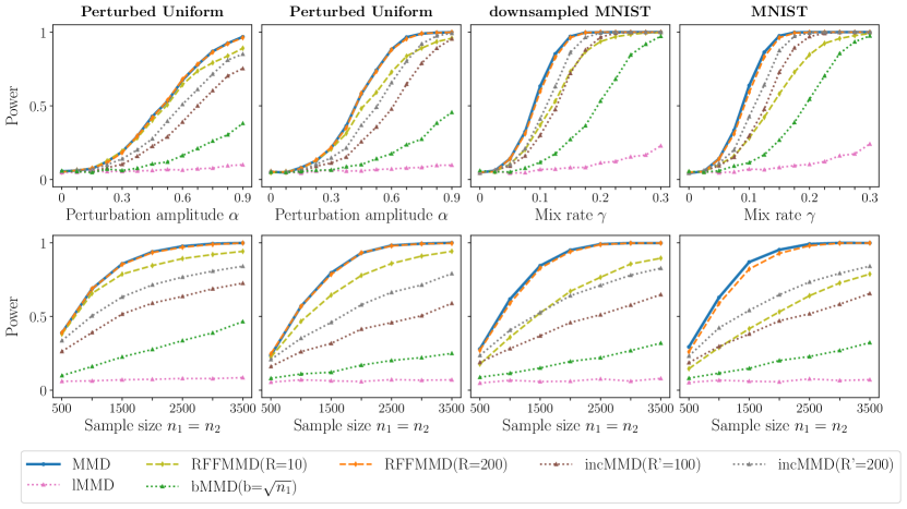
  • Scenario 3: Perturbed uniforms. Motivated by the experiments conducted in Schrab et al., (2022, 2023); Biggs et al., (2023), we investigate the test powers for capturing perturbations in uniform distributions on \mathbb{R} or 2\mathbb{R}^{2}. Specifically, for td,t\in\mathbb{R}^{d}, we set the density of the null distribution as fX(t)=𝟙[0,1](t)f_{X}(t)=\mathds{1}_{[0,1]}(t) and that of the alternative as fY(t)=𝟙[0,1](t)+αEd,p(t)f_{Y}(t)=\mathds{1}_{[0,1]}(t)+\alpha E_{d,p}(t) where α[0,p]\alpha\in[0,p] is perturbation amplitude and Ed,p(t)E_{d,p}(t) is the dd-dimensional perturbation function of size pp, defined as Ed,p(t):=p1edu{1,,p}di=1dθuG(ptiui)E_{d,p}(t):=p^{-1}e^{d}\sum_{u\in\{1,\ldots,p\}^{d}}\prod^{d}_{i=1}\theta_{u}G(pt_{i}-u_{i}) with {θu}u{1,,p}d{1,1}pd.\{\theta_{u}\}_{u\in\{1,\ldots,p\}^{d}}\in\{-1,1\}^{p^{d}}. The perturbation shape function G(t)G(t) is given by:

    G(t):=exp(11(4t+3)2)𝟙(1,12)(t)exp(11(4t+1)2)𝟙(12,0)(t),t.G(t):=\exp\left(-\frac{1}{1-(4t+3)^{2}}\right)\mathds{1}_{\left(-1,-\frac{1}{2}\right)}(t)-\exp\left(-\frac{1}{1-(4t+1)^{2}}\right)\mathds{1}_{\left(-\frac{1}{2},0\right)}(t),\quad t\in\mathbb{R}.

    We set E1,2(t)E_{1,2}(t) as an one-dimensional alternative and E2,1(t)E_{2,1}(t) as a two-dimensional alternative. In this case, the perturbation amplitude α=0\alpha=0 implies the null hypothesis and we consider different scenarios by varying α\alpha from 0 to 0.90.9. Additionally, we fix the perturbation amplitude at α=0.6\alpha=0.6 for E1,2(t)E_{1,2}(t) and α=0.45\alpha=0.45 for E2,1(t),E_{2,1}(t), and vary the sample sizes n1=n2n_{1}=n_{2}.

  • Scenario 4: MNIST. To evaluate the performance of the methods in real-world settings, we consider a task of distinguishing between the distribution of even-number images and the distribution of odd-number images in the MNIST dataset. Each data point zz is an image with dimension d=28×28=784d=28\times 28=784 (without downsampling) or d=7×7=49d=7\times 7=49 (with downsampling), with labels Lz{0,1,,9}L_{z}\in\{0,1,\ldots,9\}. We collect the images of even numbers to define a distribution Peven:={z:Lz{0,2,4,6,8}}P_{\text{even}}:=\{z:L_{z}\in\{0,2,4,6,8\}\} and collect the images of odd numbers to define another distribution Podd:={z:Lz{1,3,5,7,9}}P_{\text{odd}}:=\{z:L_{z}\in\{1,3,5,7,9\}\}. Given a mixing rate γ[0,1]\gamma\in[0,1], we set PX=PevenP_{X}=P_{\text{even}} and PY=(1γ)Peven+γPoddP_{Y}=(1-\gamma)P_{\text{even}}+\gamma P_{\text{odd}}. Accordingly, we regard the case γ=0\gamma=0 as the null hypothesis and vary γ\gamma from 0 to 0.30.3 to evaluate the power performance. When we vary the sample sizes n1=n2n_{1}=n_{2}, we fix the mixing rate at γ=0.1\gamma=0.1.

Refer to caption
Figure 1: Power experiments with two different settings: (i) univariate Gaussian distribution, (ii) high-dimensional Gaussian distribution. The sample sizes are set to n1=n2=1000{n_{1}}={n_{2}}=1000 for the first row of graphs. For the second row of graphs, parameters are set to μ=0.15\mu=0.15 in the first column, σ=1.3\sigma=1.3 in the second column, d=1000d=1000 in the third column, and σ=1.03\sigma=1.03 in the fourth column.

The simulation results for the first two scenarios are displayed in Figure 1, whereas the simulation results for the last two scenarios can be found in Figure 2. We first note that the test power of RFF-MMD test increases monotonically with RR, converging to the power of the quadratic-time MMD test. This empirically illustrates that the RFF-MMD test approximates the quadratic time MMD test as RR increases. Also, the empirical results demonstrate that different values of RR are required depending on the underlying distribution to match the power of the RFF-MMD test with that of the quadratic-time MMD test. Specifically, the RFF-MMD test matched the power of the original MMD test in all cases when R=200R=200, except in Scenario 2, where it matched when R=1000R=1000. It is also worth noting that the RFF-MMD test outperforms other efficient methods in Scenarios 1 and 3, even with RR as small as 10.

In Scenario 2, which involves a high-dimensional Gaussian setting, we observed that the power of the RFF-MMD test drops more sharply than that of the incMMD test when the sample size is fixed and the dimension increases. Conversely, when the dimension is fixed and the sample size increases, the power of the RFF-MMD test converges to that of the quadratic time MMD test more quickly than the incMMD test. A similar phenomenon was observed in Scenario 4: as the dimension increases from downsampled MNIST to MNIST data, the power curve of the RFF-MMD test shifts downward, while the power curves of other methods show little variation for the same mixing rate. However, when fixing the mixing rate and varying the sample size, the power of the RFF-MMD test increases faster than that of the incMMD test. This can be explained by the fact that the RFF-MMD test involves kernel approximation. As the dimension increases while the number of random features remains fixed, the accuracy of the kernel approximation decreases, leading to a relatively faster decline in power compared to the incMMD test. Conversely, when the dimension is fixed and the sample size varies, the incMMD test considers only a subset of the samples for computing the test statistic, resulting in a relatively slower increase in power compared to the RFF-MMD test.

Refer to caption
Figure 2: Power experiments with two different settings: (i) perturbed uniform distribution, (ii) MNIST. The sample sizes are set to n1=n2=1000{n_{1}}={n_{2}}=1000 for the first row of graphs. For the second row of graphs, parameters are set to α=0.6\alpha=0.6 in the first column, α=0.45\alpha=0.45 in the second column, and γ=0.1\gamma=0.1 in the third and last column.

We empirically measured the computational time of the considered methods under Scenario 1, as recorded in Table 1. In the experiments, we varied the sample size from 250250 to 80008000, with a mean difference of μ=0.15\mu=0.15. To ensure the efficiency of the experiments, we measured the time taken to compute the test statistic once, rather than the time taken to perform the permutation test. The results were approximated by averaging over 10001000 repetitions. From Table 1, we experimentally confirmed that while the computational time of the conventional MMD increases quadratically with the sample size, the computational times of RFF-MMD and incMMD increase linearly. Additionally, the last row of Table 1 demonstrates that the time increases linearly with the number of features, which aligns with the theoretical computational time of O(NRd)O(NRd) for RFF-MMD. We also note that similar patterns were observed in other simulation scenarios.

Table 1: Computational time (in seconds) comparisons of the considered methods under Scenario 1.
Sample
size
MMD
RFF-MMD
R=10R=10
RFF-MMD
R=200R=200
RFF-MMD
R=1000R=1000
incMMD
R=100R^{\prime}=100
incMMD
R=200R^{\prime}=200
lMMD
bMMD
b=n1/2b=n^{1/2}
250 0.0088 0.0002 0.0009 0.0070 0.0057 0.0084 0.0001 0.0006
500 0.0411 0.0003 0.0017 0.0130 0.0140 0.0251 0.0001 0.0019
1000 0.1946 0.0004 0.0051 0.0254 0.0325 0.0681 0.0002 0.0053
2000 0.7983 0.0006 0.0097 0.0485 0.0744 0.1497 0.0004 0.0155
4000 3.2662 0.0010 0.0192 0.0966 0.1567 0.3128 0.0007 0.0439
8000 13.247 0.0020 0.0371 0.1933 0.3189 0.6391 0.0015 0.1426

6 Discussion

In this work, we laid the theoretical foundations for kernel MMD tests using random Fourier features. Firstly, we proved that pointwise consistency is attainable if and only if the number of random Fourier features tends to infinity with the sample size. This observation naturally motivates an investigation into the optimal choice of the number of random Fourier features that strikes a balance between computational efficiency and statistical power. We explored this time-power trade-off under the minimax testing framework, and showed that it is possible to attain minimax separation rates within sub-quadratic time under certain distributional assumptions. We also validated these theoretical findings through numerical studies.

Our work opens up several promising avenues for future work. A natural extension of our work is to adapt our techniques to other kernel-based inference methods, such as the Hilbert–Schmidt independence criterion, and investigate fundamental time-power trade-offs in different applications. From a technical standpoint, it remains open whether a similar result to Theorem 6 can be obtained for distributions with unbounded supports. Future work can also attempt to extend our results in Section 4 to other metrics such as the Hellinger distance (e.g., Hagrass et al.,, 2022) and explore further improvements under other smoothness conditions. Finally, it would be of interest to consider deterministic Fourier features, which are shown to better approximate a kernel than random Fourier features (e.g., Wesel and Batselier,, 2021), and apply those in our application. We leave all these intriguing yet challenging problems to future work.

Acknowledgments

We acknowledge support from the Basic Science Research Program through the National Research Foundation of Korea (NRF) funded by the Ministry of Education (2022R1A4A1033384), and the Korea government (MSIT) RS-2023-00211073. We are grateful to Yongho Jeon and Gyumin Lee for their careful proofreading and helpful discussion.

References

  • Arias-Castro et al., (2018) Arias-Castro, E., Pelletier, B., and Saligrama, V. (2018). Remember the curse of dimensionality: The case of goodness-of-fit testing in arbitrary dimension. Journal of Nonparametric Statistics, 30(2):448–471.
  • Balasubramanian et al., (2021) Balasubramanian, K., Li, T., and Yuan, M. (2021). On the optimality of kernel-embedding based goodness-of-fit tests. Journal of Machine Learning Research, 22(1):1–45.
  • Baraud, (2002) Baraud, Y. (2002). Non-asymptotic minimax rates of testing in signal detection. Bernoulli, 8(5):577–606.
  • Biggs et al., (2023) Biggs, F., Schrab, A., and Gretton, A. (2023). MMD-FUSE: Learning and combining kernels for two-sample testing without data splitting. In Advances in Neural Information Processing Systems, volume 36, pages 75151–75188.
  • Bochner, (1933) Bochner, S. (1933). Monotone Funktionen, Stieltjessche Integrale und harmonische Analyse. Mathematische Annalen, 108(1):378–410.
  • Bogachev, (2007) Bogachev, V. I. (2007). Measure Theory. Springer Berlin Heidelberg.
  • Cevid et al., (2022) Cevid, D., Michel, L., Näf, J., Bühlmann, P., and Meinshausen, N. (2022). Distributional random forests: Heterogeneity adjustment and multivariate distributional regression. Journal of Machine Learning Research, 23(333):1–79.
  • Chatalic et al., (2022) Chatalic, A., Schreuder, N., Rosasco, L., and Rudi, A. (2022). Nyström kernel mean embeddings. In Proceedings of the 39th International Conference on Machine Learning, volume 162 of Proceedings of Machine Learning Research, pages 3006–3024.
  • Chatterjee and Bhattacharya, (2023) Chatterjee, A. and Bhattacharya, B. B. (2023). Boosting the power of kernel two-sample tests. arXiv preprint arXiv:2302.10687.
  • Chung and Romano, (2016) Chung, E. and Romano, J. P. (2016). Multivariate and multiple permutation tests. Journal of Econometrics, 193(1):76–91.
  • Chwialkowski et al., (2015) Chwialkowski, K. P., Ramdas, A., Sejdinovic, D., and Gretton, A. (2015). Fast two-sample testing with analytic representations of probability measures. In Advances in Neural Information Processing Systems, volume 28, pages 1981–1989.
  • Domingo-Enrich et al., (2023) Domingo-Enrich, C., Dwivedi, R., and Mackey, L. (2023). Compress then test: Powerful kernel testing in near-linear time. In International Conference on Artificial Intelligence and Statistics, volume 206 of Proceedings of Machine Learning Research, pages 1174–1218.
  • Dwivedi and Mackey, (2021) Dwivedi, R. and Mackey, L. (2021). Kernel thinning. In Proceedings of Thirty Fourth Conference on Learning Theory, volume 134 of Proceedings of Machine Learning Research, pages 1753–1753.
  • Fromont et al., (2013) Fromont, M., Laurent, B., and Reynaud-Bouret, P. (2013). The two-sample problem for Poisson processes: Adaptive tests with a nonasymptotic wild bootstrap approach. The Annals of Statistics, 41(3):1431–1461.
  • (15) Gretton, A., Borgwardt, K. M., Rasch, M. J., Schölkopf, B., and Smola, A. (2012a). A kernel two-sample test. Journal of Machine Learning Research, 13(25):723–773.
  • (16) Gretton, A., Sejdinovic, D., Strathmann, H., Balakrishnan, S., Pontil, M., Fukumizu, K., and Sriperumbudur, B. K. (2012b). Optimal kernel choice for large-scale two-sample tests. In Advances in Neural Information Processing Systems, volume 25, pages 1214–1222.
  • Guo and Shah, (2024) Guo, F. R. and Shah, R. D. (2024). Rank-transformed subsampling: inference for multiple data splitting and exchangeable p-values. arXiv preprint arXiv:2301.02739.
  • Hagrass et al., (2022) Hagrass, O., Sriperumbudur, B. K., and Li, B. (2022). Spectral regularized kernel two-sample tests. arXiv preprint arXiv:2212.09201.
  • Hemerik and Goeman, (2018) Hemerik, J. and Goeman, J. (2018). Exact testing with random permutations. Test, 27(4):811–825.
  • Ingster, (1987) Ingster, Y. I. (1987). Minimax testing of nonparametric hypotheses on a distribution density in the LpL_{p} metrics. Theory of Probability & Its Applications, 31(2):333–337.
  • Ingster, (1993) Ingster, Y. I. (1993). Asymptotically minimax hypothesis testing for nonparametric alternatives. i, ii, iii. Mathematical Methods of Statistics, 2(2):85–114.
  • Jitkrittum et al., (2016) Jitkrittum, W., Szabó, Z., Chwialkowski, K. P., and Gretton, A. (2016). Interpretable distribution features with maximum testing power. In Advances in Neural Information Processing Systems, volume 29, pages 181–189.
  • Kim, (2021) Kim, I. (2021). Comparing a large number of multivariate distributions. Bernoulli, 27(1):419–441.
  • Kim et al., (2022) Kim, I., Balakrishnan, S., and Wasserman, L. (2022). Minimax optimality of permutation tests. The Annals of Statistics, 50(1):225–251.
  • Kim and Ramdas, (2024) Kim, I. and Ramdas, A. (2024). Dimension-agnostic inference using cross U-statistics. Bernoulli, 30(1):683–711.
  • Kim and Schrab, (2023) Kim, I. and Schrab, A. (2023). Differentially private permutation tests: Applications to kernel methods. arXiv preprint arXiv:2310.19043.
  • Kirchler et al., (2020) Kirchler, M., Khorasani, S., Kloft, M., and Lippert, C. (2020). Two-sample testing using deep learning. In Proceedings of the Twenty Third International Conference on Artificial Intelligence and Statistics, volume 108 of Proceedings of Machine Learning Research, pages 1387–1398.
  • Lee, (1990) Lee, J. (1990). U-statistics: Theory and Practice. CRC Press.
  • Lehmann and Romano, (2006) Lehmann, E. and Romano, J. (2006). Testing Statistical Hypotheses. Springer New York.
  • Li and Yuan, (2019) Li, T. and Yuan, M. (2019). On the optimality of gaussian kernel based nonparametric tests against smooth alternatives. arXiv preprint arXiv:1909.03302.
  • Liu et al., (2022) Liu, F., Huang, X., Chen, Y., and Suykens, J. A. K. (2022). Random Features for Kernel Approximation: A Survey on Algorithms, Theory, and Beyond. IEEE Transactions on Pattern Analysis and Machine Intelligence, 44(10):7128–7148.
  • Liu et al., (2020) Liu, F., Xu, W., Lu, J., Zhang, G., Gretton, A., and Sutherland, D. J. (2020). Learning deep kernels for non-parametric two-sample tests. In Proceedings of the 37th International Conference on Machine Learning, volume 119 of Proceedings of Machine Learning Research, pages 6316–6326.
  • Pólya, (1949) Pólya, G. (1949). Remarks on characteristic functions. In Proceedings of the Berkeley Symposium on Mathematical Statistics and Probability, pages 115–123.
  • Rahimi and Recht, (2007) Rahimi, A. and Recht, B. (2007). Random features for large-scale kernel machines. In Advances in Neural Information Processing Systems, volume 20, pages 1177–1184.
  • Ramdas et al., (2015) Ramdas, A., Jakkam Reddi, S., Poczos, B., Singh, A., and Wasserman, L. (2015). On the decreasing power of kernel and distance based nonparametric hypothesis tests in high dimensions. Proceedings of the AAAI Conference on Artificial Intelligence, 29(1):3571–3577.
  • Romano and Siegel, (1986) Romano, J. P. and Siegel, A. F. (1986). Counterexamples in Probability and Statistics. CRC Press.
  • Schrab et al., (2023) Schrab, A., Kim, I., Albert, M., Laurent, B., Guedj, B., and Gretton, A. (2023). MMD aggregated two-sample test. Journal of Machine Learning Research, 24(194):1–81.
  • Schrab et al., (2022) Schrab, A., Kim, I., Guedj, B., and Gretton, A. (2022). Efficient Aggregated Kernel Tests using Incomplete U-statistics. In Advances in Neural Information Processing Systems, volume 35, pages 18793–18807.
  • Shekhar et al., (2023) Shekhar, S., Kim, I., and Ramdas, A. (2023). A permutation-free kernel independence test. Journal of Machine Learning Research, 24(369):1–68.
  • Sriperumbudur and Szabo, (2015) Sriperumbudur, B. and Szabo, Z. (2015). Optimal rates for random fourier features. In Advances in Neural Information Processing Systems, volume 28, page 1144–1152.
  • Sriperumbudur et al., (2010) Sriperumbudur, B. K., Gretton, A., Fukumizu, K., Schölkopf, B., and Lanckriet, G. R. (2010). Hilbert space embeddings and metrics on probability measures. Journal of Machine Learning Research, 11(50):1517–1561.
  • Stolte et al., (2023) Stolte, M., Bommert, A., and Rahnenführer, J. (2023). A Review and Taxonomy of Methods for Quantifying Dataset Similarity. arXiv preprint arXiv:2312.04078.
  • Sutherland and Schneider, (2015) Sutherland, D. J. and Schneider, J. (2015). On the error of random fourier features. In Proceedings of the Thirty-First Conference on Uncertainty in Artificial Intelligence, page 862–871.
  • Sutherland et al., (2017) Sutherland, D. J., Tung, H.-Y., Strathmann, H., De, S., Ramdas, A., Smola, A., and Gretton, A. (2017). Generative models and model criticism via optimized maximum mean discrepancy. In International Conference on Learning Representations.
  • Wesel and Batselier, (2021) Wesel, F. and Batselier, K. (2021). Large-scale learning with fourier features and tensor decompositions. In Advances in Neural Information Processing Systems, volume 34, pages 17543–17554.
  • Yamada et al., (2019) Yamada, M., Wu, D., Tsai, Y. H., Ohta, H., Salakhutdinov, R., Takeuchi, I., and Fukumizu, K. (2019). Post selection inference with incomplete maximum mean discrepancy estimator. In International Conference on Learning Representations.
  • Yao et al., (2023) Yao, J., Erichson, N. B., and Lopes, M. E. (2023). Error estimation for random fourier features. In Proceedings of The 26th International Conference on Artificial Intelligence and Statistics, volume 206 of Proceedings of Machine Learning Research, pages 2348–2364.
  • Zaremba et al., (2013) Zaremba, W., Gretton, A., and Blaschko, M. (2013). B-test: A non-parametric, low variance kernel two-sample test. In Advances in Neural Information Processing Systems, volume 26, page 755–763.
  • Zhao and Meng, (2015) Zhao, J. and Meng, D. (2015). FastMMD: Ensemble of circular discrepancy for efficient two-sample test. Neural Computation, 27(6):1345–1372.

Appendix A Technical lemmas

In this section, we collect technical lemmas used in the main proofs of our results.

Lemma 9 (Bochner,, 1933, Bochner’s theorem,).

A translation-invariant bounded continuous kernel k(x,y)=κ(xy)k(x,y)=\kappa(x-y) on d\mathbb{R}^{d} is positive definite if and only if there exists a finite non-negative Borel measure Λ\Lambda on d\mathbb{R}^{d} such that

k(x,y)=de1ω(xy)𝑑Λ(ω).k(x,y)=\int_{\mathbb{R}^{d}}e^{\sqrt{-1}\omega^{\top}(x-y)}d\Lambda(\omega).

The following result is commonly known as Young’s convolution inequality.

Lemma 10 (Bogachev,, 2007, Theorem 3.9.4).

Let pp and qq be real numbers such that 1p,q,1\leq p,q\leq\infty, 1/p+1/q=1+1/r.1/p+1/q=1+1/r. Then, for any functions fLp(d)f\in L_{p}(\mathbb{R}^{d}) and gLq(d)g\in L_{q}(\mathbb{R}^{d}),

fgrfpgq.\|f\ast g\|_{r}\leq\|f\|_{p}\|g\|_{q}.

We next collect useful asymptotic tools from Chung and Romano, (2016) to analyze the limiting behavior of permutation distributions.

Lemma 11 (Chung and Romano, 2016, Lemma A.2).

Suppose Xn=(X1,,Xn)X^{n}=(X_{1},\ldots,X_{n}) has distribution PnP_{n} in 𝒳n,\mathcal{X}_{n}, and 𝐆n\boldsymbol{G}_{n} is a finite group of transformations gg of 𝒳n\mathcal{X}_{n} onto itself. Also, let GnG_{n} be a random variable that is uniform on 𝐆n\boldsymbol{G}_{n}. Assume XnX^{n} and GnG_{n} are mutually independent. For a dd-dimensional test statistic Bn=Bn(Xn),B_{n}=B_{n}(X^{n}), let R^nB\hat{R}_{n}^{B} denote the randomization distributions of a dd-dimensional random vector Bn,B_{n}, defined by

R^nB(t)=1|𝑮n|g𝑮n𝟙{Bn(gXn)t}.\displaystyle\hat{R}^{B}_{n}(t)=\frac{1}{|\boldsymbol{G}_{n}|}\sum_{g\in\boldsymbol{G}_{n}}\mathds{1}\{B_{n}(gX^{n})\leq t\}. (12)

Suppose, under Pn,P_{n},

Bn(GnXn)𝑝b\displaystyle B_{n}(G_{n}X^{n})\xrightarrow[]{p}b (13)

for a constant bd.b\in\mathbb{R}^{d}. Then under Pn,P_{n},

R^nB(t)=1|𝑮n|g𝑮n𝟙{Bn(gXn)t}𝑝δb(t)iftb,\hat{R}^{B}_{n}(t)=\frac{1}{|\boldsymbol{G}_{n}|}\sum_{g\in\boldsymbol{G}_{n}}\mathds{1}\{B_{n}(gX^{n})\leq t\}\xrightarrow[]{p}\delta_{b}(t)\quad\text{if}~{}t\neq b,

where δc\delta_{c} denotes the distribution function corresponding to the point mass function at cd.c\in\mathbb{R}^{d}.

Lemma 12 (Chung and Romano, 2016, Lemma A.3).

Let BnB_{n} and TnT_{n} be sequences of dd-dimensional random variables satisfying Equation (13) and

(Tn(GnXn),Tn(GnXn))𝑑(T,T),(T_{n}(G_{n}X^{n}),T_{n}(G^{\prime}_{n}X^{n}))\xrightarrow{d}(T,T^{\prime}),

where TT and TT^{\prime} are independent, each with common dd-variate cumulative distribution function RT().R^{T}(\cdot). Let R^nT+B\hat{R}^{T+B}_{n}(t) denote the randomization distribution of Tn+Bn,T_{n}+B_{n}, defined in Equation (12) with BB replaced by T+B.T+B. Then, R^nT+B(t)\hat{R}^{T+B}_{n}(t) converges to the cumulative distribution function of T+bT+b in probability. In other words,

R^nT+B(t)=1|𝑮n|g𝑮n𝟙{Tn(gXn)+Bn(gXn)t}𝑝RT+b(t),\hat{R}^{T+B}_{n}(t)=\frac{1}{|\boldsymbol{G}_{n}|}\sum_{g\in\boldsymbol{G}_{n}}\mathds{1}\{T_{n}(gX^{n})+B_{n}(gX^{n})\leq t\}\xrightarrow{p}R^{T+b}(t),

if RT+bR^{T+b} is continuous at td,t\in\mathbb{R}^{d}, where RT+b()R^{T+b}(\cdot) denotes the corresponding dd-variate cumulative distribution function of T+b.T+b.

Lemma 13 (Chung and Romano, 2016, Lemma A.6).

Suppose the randomization distribution of a test statistic TnT_{n} converges to TT in probability. In other words,

R^nT(t)=1|𝑮n|g𝑮n𝟙{Tn(gXn)t}𝑝RT(t),\hat{R}^{T}_{n}(t)=\frac{1}{|\boldsymbol{G}_{n}|}\sum_{g\in\boldsymbol{G}_{n}}\mathds{1}\{T_{n}(gX^{n})\leq t\}\xrightarrow{p}R^{T}(t),

if RTR^{T} is continuous at td,t\in\mathbb{R}^{d}, where RT()R^{T}(\cdot) denotes the corresponding cumulative distribution function of tt. Let hh be a measurable map from d\mathbb{R}^{d} to s.\mathbb{R}^{s}. Let CC be the set of points in d\mathbb{R}^{d} for which hh is continuous. If (TC)=1,\mathbb{P}(T\in C)=1, then the randomization distribution of h(Tn)h(T_{n}) converges h(T)h(T) in probability.

Lemma 14 (Chung and Romano, 2016, Theorem 2.1).

Suppose that X1,,Xn1X_{1},\ldots,X_{n_{1}} are n1{n_{1}} i.i.d. random samples from the dd-dimensional distribution PXP_{X}, where Xi=(Xi,1,,Xi,d)X_{i}=(X_{i,1},\ldots,X_{i,d})^{\top} for i=1,,n1i=1,\ldots,n_{1} with mean vector μ\mu and covariance matrix ΣX\Sigma_{X} , and inedpendently, Y1,,Yn2Y_{1},\ldots,Y_{n_{2}} be n2{n_{2}} i.i.d. random samples from the dd-dimensional distribution PYP_{Y}, where Yi=(Yi,1,,Yi,d)Y_{i}=(Y_{i,1},\ldots,Y_{i,d})^{\top} for i=1,,n2i=1,\ldots,n_{2} with the common mean vector μ\mu and covariance matrix ΣY.\Sigma_{Y}. Let N=n1+n2N={n_{1}}+{n_{2}} and write Z=(Z1,,ZN)=(X1,,Xn1,Y1,,Yn2).Z=(Z_{1},\ldots,Z_{N})=(X_{1},\ldots,X_{n_{1}},Y_{1},\ldots,Y_{n_{2}}). Consider a test statistic Tn1,n2(Z1,,ZN)=n11/2[i=1n1Xin1n2j=1n2Yi]T_{{n_{1}},{n_{2}}}(Z_{1},\ldots,Z_{N})={n_{1}}^{-1/2}\big{[}\sum_{i=1}^{n_{1}}X_{i}-\frac{n_{1}}{n_{2}}\sum_{j=1}^{n_{2}}Y_{i}\big{]} and its permutation distribution

R^n1,n2T(t)=1N!π𝑮N𝟙{Tn1,n2(Zπ(1),,Zπ(N))t}\hat{R}^{T}_{{n_{1}},{n_{2}}}(t)=\frac{1}{N!}\sum_{\pi\in\boldsymbol{G}_{N}}\mathds{1}\{T_{{n_{1}},{n_{2}}}(Z_{\pi(1)},\ldots,Z_{\pi(N)})\leq t\}

where 𝐆N\boldsymbol{G}_{N} denotes the N!N! permutations of {1,2,,N}\{1,2,\ldots,N\} and tdt\in\mathbb{R}^{d^{\prime}}. Assume 0<Var(Xi,k)<0<\operatorname{Var}(X_{i,k})<\infty and 0<Var(Yj,k)<0<\operatorname{Var}(Y_{j,k})<\infty for all i=1,,n1,i=1,\ldots,{n_{1}}, j=1,,n2,j=1,\ldots,{n_{2}}, and k=1,,d.k=1,\ldots,d. Let n1,n2,{n_{1}},{n_{2}}\rightarrow\infty, p=limn1,n2n1n1+n2p=\lim_{{n_{1}},{n_{2}}\rightarrow\infty}\frac{{n_{1}}}{{n_{1}}+{n_{2}}} and assume that Σ¯=p1pΣX+ΣY\bar{\Sigma}=\frac{p}{1-p}\Sigma_{X}+\Sigma_{Y} is positive definite. Then,

suptRd|R^n1,n2T(t)G(t)|𝑝0,\sup_{t\in R^{d^{\prime}}}\big{|}\hat{R}^{T}_{{n_{1}},{n_{2}}}(t)-G(t)\big{|}\xrightarrow{p}0,

where GG denotes the dd-variate normal distribution with mean 𝟎\boldsymbol{0} and variance Σ¯.\bar{\Sigma}.

The following result is a slight modification of Ramdas et al., (2015, Proposition 1) tailored to our kernel setting.

Lemma 15 (Ramdas et al., 2015, Proposition 1).

Suppose PX=N(μ1,Σ)P_{X}=N(\mu_{1},\Sigma) and PY=N(μ2,Σ)P_{Y}=N(\mu_{2},\Sigma). The squared MMD between PXP_{X} and PYP_{Y} using a Gaussian kernel κλ(xy)=i=1d1πλiexp{(xiyi)2λi2}\kappa_{\lambda}(x-y)=\prod^{d}_{i=1}\frac{1}{\sqrt{\pi}\lambda_{i}}\exp{\bigl{\{}-\frac{(x_{i}-y_{i})^{2}}{\lambda_{i}^{2}}\bigr{\}}} has the following explicit form:

MMD2(PX,PY;k)=2(14π)d/21exp{(μXμY)(Σ+D(λ2/4))1(μXμY)/4}|Σ+D(λ2/4)|1/2,\mathrm{MMD}^{2}(P_{X},P_{Y};\mathcal{H}_{k})=2\left(\frac{1}{4\pi}\right)^{d/2}\frac{1-\exp\big{\{}-(\mu_{X}-\mu_{Y})^{\top}\left(\Sigma+D(\lambda^{2}/4)\right)^{-1}(\mu_{X}-\mu_{Y})/4\big{\}}}{\left|\Sigma+D(\lambda^{2}/4)\right|^{1/2}},

where D(λ2/4)=diag(λ12/4,,λd2/4).D(\lambda^{2}/4)=\mathrm{diag}(\lambda_{1}^{2}/4,\ldots,\lambda_{d}^{2}/4).

The next lemma facilitates the calculation of 𝔼ω[(𝔼X×Y[U1|ω])2]\mathbb{E}_{\omega}\big{[}\big{(}\mathbb{E}_{X\times Y}[U_{1}\,|\,\omega]\big{)}^{2}\big{]}. The proof can be found in Appendix B.8.

Lemma 16.

Let X,X′′X^{\prime},X^{\prime\prime} and Y,Y′′Y^{\prime},Y^{\prime\prime} be the independent copies of XX and YY, respectively. Then, the following two equations hold:

𝔼ω[(𝔼X×Y[U1|ω])2]\displaystyle\mathbb{E}_{\omega}\big{[}\big{(}\mathbb{E}_{X\times Y}[U_{1}\,|\,\omega]\big{)}^{2}\big{]} =2κ(0)MMD2(PXX,PX′′Y;k)+2κ(0)MMD2(PYY,PXY′′;k)\displaystyle=2\kappa(0)\mathrm{MMD}^{2}(P_{X-X^{\prime}},P_{X^{\prime\prime}-Y};\mathcal{H}_{k})+2\kappa(0)\mathrm{MMD}^{2}(P_{Y-Y^{\prime}},P_{X-Y^{\prime\prime}};\mathcal{H}_{k})
κ(0)MMD2(PX+X,PY+Y;k)and\displaystyle\quad-\kappa(0)\mathrm{MMD}^{2}(P_{X+X^{\prime}},P_{Y+Y^{\prime}};\mathcal{H}_{k})\quad\text{and}
𝔼ω[(𝔼X×Y[U1|ω])2]\displaystyle\mathbb{E}_{\omega}\big{[}\big{(}\mathbb{E}_{X\times Y}[U_{1}\,|\,\omega]\big{)}^{2}\big{]} =2κ(0)MMD2(PX+X,PX′′+Y;k)+2κ(0)MMD2(PY+Y,PX+Y′′;k)\displaystyle=2\kappa(0)\mathrm{MMD}^{2}(P_{X+X^{\prime}},P_{X^{\prime\prime}+Y};\mathcal{H}_{k})+2\kappa(0)\mathrm{MMD}^{2}(P_{Y+Y^{\prime}},P_{X+Y^{\prime\prime}};\mathcal{H}_{k})
κ(0)MMD2(PX+X,PY+Y;k).\displaystyle\quad-\kappa(0)\mathrm{MMD}^{2}(P_{X+X^{\prime}},P_{Y+Y^{\prime}};\mathcal{H}_{k}).

The next lemma serve as a main block in the proof of Propositions 8. The proof can be found in Appendix B.9.

Lemma 17.

For the class of distribution pairs, 𝒞N,Σ\mathcal{C}_{N,\Sigma}, in Equation (11) and the Gaussian kernel kλ(x,y)k_{\lambda}(x,y) with any fixed bandwidth λ=(λ1,,λd)(0,)d\lambda=(\lambda_{1},\ldots,\lambda_{d})^{\top}\in(0,\infty)^{d}, the inequality in Equation (10) holds with c=2c=2. Specifically, there exists a constant C=C(d,λ,Σ)>0C=C(d,\lambda,\Sigma)>0 such that

𝔼ω[(𝔼X×Y[U1|ω])2]\displaystyle\mathbb{E}_{\omega}\big{[}\big{(}\mathbb{E}_{X\times Y}[U_{1}\,|\,\omega]\big{)}^{2}\big{]} C(𝔼ω[𝔼X×Y[U1|ω]])c=C(d,λ,Σ)(MMD2(PX,PY;k))2.\displaystyle\leq C\big{(}\mathbb{E}_{\omega}\big{[}\mathbb{E}_{X\times Y}[U_{1}\,|\,\omega]\big{]}\big{)}^{c}=C(d,\lambda,\Sigma)\big{(}\mathrm{MMD}^{2}(P_{X},P_{Y};\mathcal{H}_{k})\big{)}^{2}.
Remark 17.1.

Regarding the range of c(1,2]c\in(1,2] in Equation (10), note that when c>2c>2, the inequality in Equation (10) yields MMD1\mathrm{MMD}\gtrsim 1 and this is not of our interest (in fact, this condition becomes vacuous since MMD\mathrm{MMD} using a bounded kernel is bounded above by a constant). More specifically, by Jensen’s inequality, we have MMD4𝔼ω[(𝔼X×Y[U1|ω])2]\mathrm{MMD}^{4}\leq\mathbb{E}_{\omega}\big{[}\big{(}\mathbb{E}_{X\times Y}[U_{1}\,|\,\omega]\big{)}^{2}\big{]} and then the inequality in Equation (10) implies

MMD4(PX,PY;kλ)CMMD2c(PX,PY;kλ)\displaystyle\mathrm{MMD}^{4}(P_{X},P_{Y};\mathcal{H}_{k_{\lambda}})\leq C\mathrm{MMD}^{2c}(P_{X},P_{Y};\mathcal{H}_{k_{\lambda}})
\displaystyle\equiv~{} MMD2(2c)(PX,PY;kλ)C\displaystyle\mathrm{MMD}^{2(2-c)}(P_{X},P_{Y};\mathcal{H}_{k_{\lambda}})\leq C
\displaystyle\equiv~{} 1C12(c2)=CMMD(PX,PY;kλ).\displaystyle\frac{1}{C^{\frac{1}{2(c-2)}}}=C^{\prime}\leq\mathrm{MMD}(P_{X},P_{Y};\mathcal{H}_{k_{\lambda}}).

Therefore we may see some computational gain when c>2c>2 but it is only possible when the minimum separation is of constant order as MMD1\mathrm{MMD}\gtrsim 1.

Appendix B Proofs

Notation and terminology.

We start by organizing the notation and the terminology we use throughout this appendix. Unless explicitly stated otherwise, the symbol ()\mathbb{P}(\cdot) denotes the probability measure that takes into account all inherent uncertainties. In addition, we represent constants as C1,C2,C_{1},C_{2},\ldots, which may depend on “fixed” parameters such as M1,M2,M3,α,β,d,sM_{1},M_{2},M_{3},\alpha,\beta,d,s that do not vary with the sample sizes n1{n_{1}} and n2{n_{2}}. The specific values of these constants may vary in different places. We use the notation An𝑝AA_{n}\xrightarrow{p}A to denote that the sequence of the random variables AnA_{n} converges in probability to a random variable A.A. We also introduce a terminology for the convergence of permutation distributions. For a given generic test statistic Tn1,n2T_{{n_{1}},{n_{2}}} and a continuous random variable GG, denote the permutation distribution of Tn1,n2T_{{n_{1}},{n_{2}}} as FTn1,n2π():=1N!πΠN𝟙{Tn1,n2(Zπ(1),,Zπ(N))}F^{\pi}_{T_{{n_{1}},{n_{2}}}}(\cdot):=\frac{1}{N!}\sum_{\pi\in\Pi_{N}}\mathds{1}\{T_{{n_{1}},{n_{2}}}(Z_{\pi(1)},\dots,Z_{\pi(N)})\leq\cdot\} and the cumulative distribution function (CDF) of GG as FG():=(G)F_{G}(\cdot):=\mathbb{P}(G\leq\cdot). Suppose that

suptd|FTn1,n2π(t)FG(t)|𝑝0,\sup_{t\in\mathbb{R}^{d}}\big{|}F^{\pi}_{T_{{n_{1}},{n_{2}}}}(t)-F_{G}(t)\big{|}\xrightarrow{p}0,

or equivalently, for any given ϵ>0,\epsilon>0,

limn1,n2(suptd|FTn1,n2π(t)FG(t)|>ϵ)=0.\lim_{{n_{1}},{n_{2}}\rightarrow\infty}\mathbb{P}\bigg{(}\sup_{t\in\mathbb{R}^{d}}\big{|}F^{\pi}_{T_{{n_{1}},{n_{2}}}}(t)-F_{G}(t)\big{|}>\epsilon\bigg{)}=0.

In this case, we say that FTn1,n2πF^{\pi}_{T_{{n_{1}},{n_{2}}}} converges weakly in probability to GG, as in Chung and Romano, (2016). Also, if a sequence of random variables {Hn}n=1\{H_{n}\}_{n=1}^{\infty} converges in distribution to a continuous random variable HH, we use the expression that aligns with the above:

suptd|FHn(t)FH(t)|0,\sup_{t\in\mathbb{R}^{d}}\big{|}F_{H_{n}}(t)-F_{H}(t)\big{|}\rightarrow 0,

instead of Hn𝑑H.H_{n}\xrightarrow{d}H. Note that Pólya’s theorem can be generalized into the multivariate case (Guo and Shah,, 2024, Lemma C.7) and thus guarantees the equivalence between those two expressions under the assumption that HH is continuous.

B.1 Proof of Proposition 2

For simplicity, we consider the case where d=1d=1, as the scenario with d2d\geq 2 can be extended naturally by taking the Cartesian product of the one-dimensional cases. Also, we consider the case k=2k=2, since the case k=1k=1 is identical to Lemma 1, and the logic used for k=2k=2 can be extended to prove the cases for k3k\geq 3.

Now, suppose that k=2k=2. Given frequencies 𝝎R={ω1,,ωR},\boldsymbol{\omega}_{R}=\{\omega_{1},\ldots,\omega_{R}\}, recall that the feature mapping is defined as

𝝍𝝎R(x)=[cos(ω1x),sin(ω1x),,cos(ωRx),sin(ωRx)]2R,\boldsymbol{\psi}_{\boldsymbol{\omega}_{R}}(x)=[\cos(\omega_{1}^{\top}x),\sin(\omega_{1}^{\top}x),~{}\ldots~{},\cos(\omega_{R}^{\top}x),\sin(\omega_{R}^{\top}x)]^{\top}\in\mathbb{R}^{2R},

and 2\mathcal{E}_{2} can be written as

2:={𝒙d×R:𝔼X[𝝍𝒙(X)]=𝔼Y[𝝍𝒙(Y)],𝔼X[𝝍𝒙(X)𝝍𝒙(X)]=𝔼Y[𝝍𝒙(Y)𝝍𝒙(Y)]}.\mathcal{E}_{2}:=\bigl{\{}\boldsymbol{x}\in\mathbb{R}^{d\times R}:\mathbb{E}_{X}[\boldsymbol{\psi}_{\boldsymbol{x}}(X)]=\mathbb{E}_{Y}[\boldsymbol{\psi}_{\boldsymbol{x}}(Y)],~{}\mathbb{E}_{X}[\boldsymbol{\psi}_{\boldsymbol{x}}(X)\boldsymbol{\psi}_{\boldsymbol{x}}(X)^{\top}]=\mathbb{E}_{Y}[\boldsymbol{\psi}_{\boldsymbol{x}}(Y)\boldsymbol{\psi}_{\boldsymbol{x}}(Y)^{\top}]\bigr{\}}.

Then, the components of the second moment matrix of 𝝍𝝎R(X)\boldsymbol{\psi}_{\boldsymbol{\omega}_{R}}(X) should be one of the following terms:

𝔼X[cos(ωiX)cos(ωjX)],\displaystyle\mathbb{E}_{X}[\cos(\omega_{i}^{\top}X)\cos(\omega_{j}^{\top}X)], i,j=1,,R,or\displaystyle\quad i,j=1,\ldots,R,\quad\text{or}
𝔼X[cos(ωiX)sin(ωjX)],\displaystyle\mathbb{E}_{X}[\cos(\omega_{i}^{\top}X)\sin(\omega_{j}^{\top}X)], i,j=1,,R,or\displaystyle\quad i,j=1,\ldots,R,\quad\text{or}
𝔼X[sin(ωiX)sin(ωjX)],\displaystyle\mathbb{E}_{X}[\sin(\omega_{i}^{\top}X)\sin(\omega_{j}^{\top}X)], i,j=1,,R.\displaystyle\quad i,j=1,\ldots,R.

Similarly, the same argument holds true for 𝝍𝝎R(Y)\boldsymbol{\psi}_{\boldsymbol{\omega}_{R}}(Y). Hence, to show that 𝔼X[𝝍𝝎R(X)𝝍𝝎R(X)]=𝔼Y[𝝍𝒙(Y)𝝍𝒙(Y)]\mathbb{E}_{X}[\boldsymbol{\psi}_{\boldsymbol{\omega}_{R}}(X)\boldsymbol{\psi}_{\boldsymbol{\omega}_{R}}(X)^{\top}]=\mathbb{E}_{Y}[\boldsymbol{\psi}_{\boldsymbol{x}}(Y)\boldsymbol{\psi}_{\boldsymbol{x}}(Y)^{\top}] holds, it is enough to show that the following identities are satisfied simultaneously:

𝔼X[cos(ωiX)cos(ωjX)]\displaystyle\mathbb{E}_{X}[\cos(\omega_{i}^{\top}X)\cos(\omega_{j}^{\top}X)] =𝔼Y[cos(ωiY)cos(ωjY)],\displaystyle=\mathbb{E}_{Y}[\cos(\omega_{i}^{\top}Y)\cos(\omega_{j}^{\top}Y)],
𝔼X[cos(ωiX)sin(ωjX)]\displaystyle\mathbb{E}_{X}[\cos(\omega_{i}^{\top}X)\sin(\omega_{j}^{\top}X)] =𝔼Y[cos(ωiY)sin(ωjY)],\displaystyle=\mathbb{E}_{Y}[\cos(\omega_{i}^{\top}Y)\sin(\omega_{j}^{\top}Y)],
𝔼X[sin(ωiX)sin(ωjX)]\displaystyle\mathbb{E}_{X}[\sin(\omega_{i}^{\top}X)\sin(\omega_{j}^{\top}X)] =𝔼Y[sin(ωiY)sin(ωjY)],\displaystyle=\mathbb{E}_{Y}[\sin(\omega_{i}^{\top}Y)\sin(\omega_{j}^{\top}Y)],

for all i,j=1,,R.i,j=1,\ldots,R. By trigonometric identities, these identities are equivalent to

𝔼X[cos((ωiωj)X)+cos((ωi+ωj)X)]\displaystyle\mathbb{E}_{X}\big{[}\cos\big{(}(\omega_{i}-\omega_{j})^{\top}X\big{)}+\cos\big{(}(\omega_{i}+\omega_{j})^{\top}X\big{)}\big{]} =𝔼Y[cos((ωiωj)Y)+cos((ωi+ωj)Y)],\displaystyle=\mathbb{E}_{Y}\big{[}\cos\big{(}(\omega_{i}-\omega_{j})^{\top}Y\big{)}+\cos\big{(}(\omega_{i}+\omega_{j})^{\top}Y\big{)}\big{]},
𝔼X[sin((ωi+ωj)X)sin((ωiωj)X)]\displaystyle\mathbb{E}_{X}\big{[}\sin\big{(}(\omega_{i}+\omega_{j})^{\top}X\big{)}-\sin\big{(}(\omega_{i}-\omega_{j})^{\top}X\big{)}\big{]} =𝔼Y[sin((ωi+ωj)Y)sin((ωiωj)Y)],\displaystyle=\mathbb{E}_{Y}\big{[}\sin\big{(}(\omega_{i}+\omega_{j})^{\top}Y\big{)}-\sin\big{(}(\omega_{i}-\omega_{j})^{\top}Y\big{)}\big{]},
𝔼X[cos((ωiωj)X)cos((ωi+ωj)X)]\displaystyle\mathbb{E}_{X}\big{[}\cos\big{(}(\omega_{i}-\omega_{j})^{\top}X\big{)}-\cos\big{(}(\omega_{i}+\omega_{j})^{\top}X\big{)}\big{]} =𝔼Y[cos((ωiωj)Y)cos((ωi+ωj)Y)],\displaystyle=\mathbb{E}_{Y}\big{[}\cos\big{(}(\omega_{i}-\omega_{j})^{\top}Y\big{)}-\cos\big{(}(\omega_{i}+\omega_{j})^{\top}Y\big{)}\big{]},

for all i,j=1,,R.i,j=1,\ldots,R. Hence, if we show that the following identities

𝔼X[cos((ωi+ωj)X)]\displaystyle\mathbb{E}_{X}\big{[}\cos\big{(}(\omega_{i}+\omega_{j})^{\top}X\big{)}\big{]} =𝔼Y[cos((ωi+ωj)Y)],\displaystyle=\mathbb{E}_{Y}\big{[}\cos\big{(}(\omega_{i}+\omega_{j})^{\top}Y\big{)}\big{]},
𝔼X[sin((ωi+ωj)X)]\displaystyle\mathbb{E}_{X}\big{[}\sin\big{(}(\omega_{i}+\omega_{j})^{\top}X\big{)}\big{]} =𝔼Y[sin((ωi+ωj)Y)],\displaystyle=\mathbb{E}_{Y}\big{[}\sin\big{(}(\omega_{i}+\omega_{j})^{\top}Y\big{)}\big{]},
𝔼X[cos((ωiωj)X)]\displaystyle\mathbb{E}_{X}\big{[}\cos\big{(}(\omega_{i}-\omega_{j})^{\top}X\big{)}\big{]} =𝔼Y[cos((ωiωj)Y)],\displaystyle=\mathbb{E}_{Y}\big{[}\cos\big{(}(\omega_{i}-\omega_{j})^{\top}Y\big{)}\big{]},
𝔼X[sin((ωiωj)X)]\displaystyle\mathbb{E}_{X}\big{[}\sin\big{(}(\omega_{i}-\omega_{j})^{\top}X\big{)}\big{]} =𝔼Y[sin((ωiωj)Y)]\displaystyle=\mathbb{E}_{Y}\big{[}\sin\big{(}(\omega_{i}-\omega_{j})^{\top}Y\big{)}\big{]}

hold for all i,j=1,,Ri,j=1,\ldots,R given 𝝎R,\boldsymbol{\omega}_{R}, the second moment matrices of 𝝍𝝎R(X)\boldsymbol{\psi}_{\boldsymbol{\omega}_{R}}(X) and 𝝍𝝎R(Y)\boldsymbol{\psi}_{\boldsymbol{\omega}_{R}}(Y) become identical. Also, note that satisfying the first two identities is equivalent to the coincidence of characteristic functions ϕX(ω)\phi_{X}(\omega) and ϕY(ω)\phi_{Y}(\omega) at the point ωi+ωj,\omega_{i}+\omega_{j}, and the last two identities imply the coincidence of ϕX(ω)\phi_{X}(\omega) and ϕY(ω)\phi_{Y}(\omega) at the point ωiωj.\omega_{i}-\omega_{j}. Let us denote ωi+ωj\omega_{i}+\omega_{j} and ωiωj\omega_{i}-\omega_{j} as ωiR+j\omega_{iR+j} and ω2iR+j\omega_{2iR+j}, respectively, for all i,j=1,,Ri,j=1,\ldots,R, and then, a sufficient condition for 𝝎R2\boldsymbol{\omega}_{R}\in\mathcal{E}_{2} is ϕX(ωr)=ϕY(ωr)\phi_{X}(\omega_{r})=\phi_{Y}(\omega_{r}) for all r=1,,2R2+R.r=1,\ldots,2R^{2}+R. Now, observe that all random variables {ωr}r=12R2+R\{\omega_{r}\}^{2R^{2}+R}_{r=1} have continuous probability distributions, and thus, for any ϵ>0\epsilon>0, we can find I=I(ϵ)>0I=I(\epsilon)>0 satisfying (ωr[I,I])(2R2+R)1ϵ\mathbb{P}(\omega_{r}\in[-I,I])\leq(2R^{2}+R)^{-1}\epsilon for all r=1,,2R2+R.r=1,\ldots,2R^{2}+R. Then,

(ω1,,ω2R2+R[I,I]c)\displaystyle\mathbb{P}(\omega_{1},\ldots,\omega_{2R^{2}+R}\in[-I,I]^{c}) 1r=12R2+R(ωr[I,I])\displaystyle\geq 1-\sum^{2R^{2}+R}_{r=1}\mathbb{P}(\omega_{r}\in[-I,I])
1ϵ.\displaystyle\geq 1-\epsilon.

Here, according to Pólya’s criterion (Pólya,, 1949, Theorem 1), we can find uncountably many characteristic functions that vanish outside the interval [I,I],[-I,I], and let us denote this set as 𝒜k,ϵ.\mathcal{A}_{k,\epsilon}. A representative example of these functions (see e.g., Chwialkowski et al.,, 2015, Proposition 1) is a set {fδ}δ>I1\{f_{\delta}\}_{\delta>I^{-1}} where

fδ(ω)={1δ|ω| when |ω|1δ,0 when |ω|1δ.\displaystyle f_{\delta}(\omega)=\left\{\begin{array}[]{lll}1-\delta|\omega|&\text{ when }&|\omega|\leq\frac{1}{\delta},\\[5.0pt] 0&\text{ when }&|\omega|\geq\frac{1}{\delta}.\end{array}\right.

Then, for any distribution pair PX,PY𝒜k,ϵ,P_{X},P_{Y}\in\mathcal{A}_{k,\epsilon}, we have

𝝎R(𝝎R2)\displaystyle\mathbb{P}_{\boldsymbol{\omega}_{R}}(\boldsymbol{\omega}_{R}\in\mathcal{E}_{2}) (ω1,,ω2R2+R[I,I]c)\displaystyle\geq\mathbb{P}(\omega_{1},\ldots,\omega_{2R^{2}+R}\in[-I,I]^{c})
1r=12R2+R(ωr[I,I])\displaystyle\geq 1-\sum^{2R^{2}+R}_{r=1}\mathbb{P}(\omega_{r}\in[-I,I])
1ϵ,\displaystyle\geq 1-\epsilon,

and this completes the proof.

B.2 Proof of Theorem 3

Recall that we use a permutation test defined as follows:

Δn1,n2,Rα:=𝟙(V>qn1,n2,1α).\Delta_{{n_{1}},{n_{2}},R}^{\alpha}:=\mathds{1}(V>q_{{n_{1}},{n_{2}},1-\alpha}).

We first note that the permutation test is invariant under multiplying a positive constant n1{n_{1}} to the test statistic. Therefore, throughout the proof of Theorem 3, we consider n1V{n_{1}}V as a test statistic and its permutation quantile n1qn1,n2,1α{n_{1}}q_{{n_{1}},{n_{2}},1-\alpha} instead of VV and qn1,n2,1αq_{{n_{1}},{n_{2}},1-\alpha}, respectively. Now, note that both the test statistic n1V{n_{1}}V and the permutation quantile n1qn1,n2,1α{n_{1}}q_{{n_{1}},{n_{2}},1-\alpha} are random variables. Our strategy to prove Theorem 3 is to first assume the ME condition (7), 𝝎R\boldsymbol{\omega}_{R}\in\mathcal{E}, which holds for any distribution pair PX,PY𝒜ϵP_{X},P_{Y}\in\mathcal{A}_{\epsilon} with high probability by Lemma 1. For such fixed 𝝎R\boldsymbol{\omega}_{R}, we analyze the asymptotic behavior of n1V{n_{1}}V and show that the test power is strictly smaller than one for an uncountable number of pairs of distributions PXP_{X} and PYP_{Y}.

Asymptotic behavior of the unconditional distribution

Let us start by investigating the test statistic n1V{n_{1}}V with a fixed 𝝎R\boldsymbol{\omega}_{R}\in\mathcal{E}. For the sake of notation, we denote the covariances of 𝝍𝝎R(X)\boldsymbol{\psi}_{\boldsymbol{\omega}_{R}}(X) and 𝝍𝝎R(Y)\boldsymbol{\psi}_{\boldsymbol{\omega}_{R}}(Y) as Σ𝝍𝝎R(X)\Sigma_{\boldsymbol{\psi}_{\boldsymbol{\omega}_{R}}(X)} and Σ𝝍𝝎R(Y)\Sigma_{\boldsymbol{\psi}_{\boldsymbol{\omega}_{R}}(Y)}, respectively. Note that 𝝍𝝎R(X)\boldsymbol{\psi}_{\boldsymbol{\omega}_{R}}(X) and 𝝍𝝎R(Y)\boldsymbol{\psi}_{\boldsymbol{\omega}_{R}}(Y) are trigonometric functions, having finite variance. Hence the central limit theorem guarantees that the unconditional distribution of n11/2T{n_{1}}^{1/2}T converges in distribution to N(0,Σ~)N(0,\tilde{\Sigma}) where Σ~=Σ𝝍𝝎R(X)+p1pΣ𝝍𝝎R(Y)2R×2R\tilde{\Sigma}=\Sigma_{\boldsymbol{\psi}_{\boldsymbol{\omega}_{R}}(X)}+\frac{p}{1-p}\Sigma_{\boldsymbol{\psi}_{\boldsymbol{\omega}_{R}}(Y)}\in\mathbb{R}^{2R\times 2R}. Letting k~=rank(Σ~)\tilde{k}=\operatorname{rank}(\tilde{\Sigma}), consider an eigendecomposition of Σ~\tilde{\Sigma}:

Σ~=Q~D~Q~.\tilde{\Sigma}=\tilde{Q}\tilde{D}\tilde{Q}^{\top}.

Here, D~=diag(λ~1,,λ~k~)k~×k~\tilde{D}=\mathrm{diag}(\tilde{\lambda}_{1},\ldots,\tilde{\lambda}_{\tilde{k}})\in\mathbb{R}^{\tilde{k}\times\tilde{k}} is a diagonal matrix formed from the non-zero eigenvalues of Σ~\tilde{\Sigma}, and Q~2R×k~\tilde{Q}\in\mathbb{R}^{2R\times\tilde{k}} is an orthogonal matrix with columns corresponding to the eigenvectors of Σ~\tilde{\Sigma}. Then, a Gaussian random vector AN(0,Σ~)A\sim N(0,\tilde{\Sigma}) can be decomposed as A=Q~D12GA=\tilde{Q}D^{\frac{1}{2}}G where G=(G1,,Gk~)N(0,Ik~×k~)G=(G_{1},\ldots,G_{\tilde{k}})^{\top}\sim N(0,I_{\tilde{k}\times\tilde{k}}). Therefore, the distribution of Ak~2\|A\|^{2}_{\mathbb{R}^{\tilde{k}}} can be derived as follows:

Ak~2=AA\displaystyle\|A\|^{2}_{\mathbb{R}^{\tilde{k}}}=A^{\top}A =GD~12Q~Q~D~12G=GD~12D~12G\displaystyle=G^{\top}\tilde{D}^{\frac{1}{2}}\tilde{Q}^{\top}\tilde{Q}\tilde{D}^{\frac{1}{2}}G=G^{\top}\tilde{D}^{\frac{1}{2}}\tilde{D}^{\frac{1}{2}}G
=i=1k~λ~iGi2.\displaystyle=\sum^{\tilde{k}}_{i=1}\tilde{\lambda}_{i}G^{2}_{i}.

Based on the fact that n11/2T{n_{1}}^{1/2}T converges in distribution to AA, the continuous mapping theorem guarantees

suptd|Fn1V(t)Fλ~iGi2(t)|0\sup_{t\in\mathbb{R}^{d}}\big{|}F_{{n_{1}}V}(t)-F_{\sum\tilde{\lambda}_{i}G_{i}^{2}}(t)\big{|}\rightarrow 0 (14)

for fixed 𝝎R\boldsymbol{\omega}_{R}\in\mathcal{E}, where Fλ~iGi2F_{\sum\tilde{\lambda}_{i}G_{i}^{2}} is the CDF of i=1k~λ~iGi2.\sum^{\tilde{k}}_{i=1}\tilde{\lambda}_{i}G_{i}^{2}. If k~=2R\tilde{k}=2R, then the limiting distribution becomes i=12Rλ~iGi2\sum^{2R}_{i=1}\tilde{\lambda}_{i}G_{i}^{2}. Even when k~\tilde{k} is strictly less than 2R2R, we note that the distribution Fλ~iGi2F_{\sum\tilde{\lambda}_{i}G_{i}^{2}} can also be regarded as the distribution of i=12Rλ~iGi2\sum^{2R}_{i=1}\tilde{\lambda}_{i}G_{i}^{2} instead of i=1k~λ~iGi2,\sum^{\tilde{k}}_{i=1}\tilde{\lambda}_{i}G_{i}^{2}, since we can extend the eigenvalue set {λ~i}i=1k~\{\tilde{\lambda}_{i}\}_{i=1}^{\tilde{k}} to {λ~i}i=12R\{\tilde{\lambda}_{i}\}_{i=1}^{2R} by including zero eigenvalues.

Asymptotic behavior of the permutation distribution

We now examine the asymptotic behavior of the permutation distribution of n1V{n_{1}}V and n1qn1,n2,1α{n_{1}}q_{{n_{1}},{n_{2}},1-\alpha} for fixed 𝝎R\boldsymbol{\omega}_{R}\in\mathcal{E}. First, let k¯=rank(Σ¯)\bar{k}=\operatorname{rank}(\bar{\Sigma}) where Σ¯=p1pΣ𝝍𝝎R(X)+Σ𝝍𝝎R(Y)\bar{\Sigma}=\frac{p}{1-p}\Sigma_{\boldsymbol{\psi}_{\boldsymbol{\omega}_{R}}(X)}+\Sigma_{\boldsymbol{\psi}_{\boldsymbol{\omega}_{R}}(Y)}, and consider an eigendecomposition

Σ¯\displaystyle\bar{\Sigma} =QDQ=[Q¯|Q0][D¯𝟎𝟎𝟎][Q¯|Q0]\displaystyle=QDQ^{\top}=\left[\bar{Q}\,|\,Q_{0}\right]\left[\begin{array}[]{c|c}\bar{D}&\mathbf{0}\\ \hline\cr\mathbf{0}&\mathbf{0}\end{array}\right]\left[\bar{Q}\,|\,Q_{0}\right]^{\top}
=Q¯D¯Q¯,\displaystyle=\bar{Q}\bar{D}\bar{Q}^{\top},

where D2R×2RD\in\mathbb{R}^{2R\times 2R} is a diagonal matrix composed of D¯\bar{D} and zeros, D¯=diag(λ¯1,,λ¯k¯)k¯×k¯\bar{D}=\text{diag}(\bar{\lambda}_{1},\ldots,\bar{\lambda}_{\bar{k}})\in\mathbb{R}^{\bar{k}\times\bar{k}} is a diagonal matrix formed from the non-zero eigenvalues of Σ¯\bar{\Sigma}. In addition Q¯2R×k¯\bar{Q}\in\mathbb{R}^{2R\times\bar{k}} denotes an orthogonal matrix whose columns are the eigenvectors of Σ¯\bar{\Sigma} and Q02R×(2Rk¯)Q_{0}\in\mathbb{R}^{2R\times(2R-\bar{k})} denotes an orthogonal matrix that makes Q=[Q¯|Q0]2R×2RQ=\left[\bar{Q}\,|\,Q_{0}\right]\in\mathbb{R}^{2R\times 2R} also orthogonal. Note that n1V{n_{1}}V can be decomposed as

n1V\displaystyle{n_{1}}V =n1TT\displaystyle={n_{1}}T^{\top}T (15)
=n1TQQT\displaystyle={n_{1}}T^{\top}QQ^{\top}T
=n1TQ¯Q¯T+n1TQ0Q0T.\displaystyle={n_{1}}T^{\top}\bar{Q}\bar{Q}^{\top}T+{n_{1}}T^{\top}Q_{0}Q_{0}^{\top}T.

For the first term, note that Q¯T=1n1i=1n1Q¯𝝍𝝎R(Xi)1n2j=1n2Q¯𝝍𝝎R(Yj)\bar{Q}^{\top}T=\frac{1}{n_{1}}\sum_{i=1}^{n_{1}}\bar{Q}^{\top}\boldsymbol{\psi}_{\boldsymbol{\omega}_{R}}(X_{i})-\frac{1}{{n_{2}}}\sum_{j=1}^{n_{2}}\bar{Q}^{\top}\boldsymbol{\psi}_{\boldsymbol{\omega}_{R}}(Y_{j}) and 𝔼X[Q¯𝝍𝝎R(X)]=𝔼YQ[Q¯𝝍𝝎R(Y)]\mathbb{E}_{X}[\bar{Q}^{\top}\boldsymbol{\psi}_{\boldsymbol{\omega}_{R}}(X)]=\mathbb{E}_{Y\sim Q}[\bar{Q}^{\top}\boldsymbol{\psi}_{\boldsymbol{\omega}_{R}}(Y)] for 𝝎R\boldsymbol{\omega}_{R}\in\mathcal{E}. Furthermore, we observe that

p1pΣQ¯𝝍𝝎R(X)+ΣQ¯𝝍𝝎R(Y)\displaystyle\frac{p}{1-p}\Sigma_{\bar{Q}\boldsymbol{\psi}_{\boldsymbol{\omega}_{R}}(X)}+\Sigma_{\bar{Q}\boldsymbol{\psi}_{\boldsymbol{\omega}_{R}}(Y)} =p1pQ¯Σ𝝍𝝎R(X)Q¯+Q¯Σ𝝍𝝎R(Y)Q¯\displaystyle=\frac{p}{1-p}\bar{Q}^{\top}\Sigma_{\boldsymbol{\psi}_{\boldsymbol{\omega}_{R}}(X)}\bar{Q}+\bar{Q}^{\top}\Sigma_{\boldsymbol{\psi}_{\boldsymbol{\omega}_{R}}(Y)}\bar{Q}
=Q¯(p1pΣ𝝍𝝎R(X)+Σ𝝍𝝎R(Y))Q¯\displaystyle=\bar{Q}^{\top}\Big{(}\frac{p}{1-p}\Sigma_{\boldsymbol{\psi}_{\boldsymbol{\omega}_{R}}(X)}+\Sigma_{\boldsymbol{\psi}_{\boldsymbol{\omega}_{R}}(Y)}\Big{)}\bar{Q}
=Q¯Σ¯Q¯\displaystyle=\bar{Q}^{\top}\bar{\Sigma}\bar{Q}
=D¯.\displaystyle=\bar{D}.

Since D¯\bar{D} is positive definite, we apply Lemma 14 to n11/2Q¯T{n_{1}}^{1/2}\bar{Q}^{\top}T and conclude that the permutation distribution of n11/2Q¯{n_{1}}^{1/2}\bar{Q}^{\top} converges weakly in probability to N(0,D¯)N(0,\bar{D}) for fixed 𝝎R\boldsymbol{\omega}_{R}\in\mathcal{E}. Therefore, the continuous mapping theorem for permutation distribution (Chung and Romano,, 2016, Lemma A.6) guarantees that the permutation distribution of n1TQ¯Q¯T{n_{1}}T^{\top}\bar{Q}\bar{Q}^{\top}T converges weakly in probability to i=1k¯λ¯iGi2\sum^{\bar{k}}_{i=1}\bar{\lambda}_{i}G_{i}^{2} for 𝝎R\boldsymbol{\omega}_{R}\in\mathcal{E}. More formally, if we denote the permutation distribution of n1TQ¯Q¯T{n_{1}}T^{\top}\bar{Q}\bar{Q}^{\top}T as F(n11/2Q¯T)2π(t)F^{\pi}_{({n_{1}}^{1/2}\bar{Q}T)^{2}}(t), for any ϵ>0,\epsilon>0, we have

limn1,n2(supt|F(n11/2Q¯T)2π(t)Fλ¯iGi2(t)|>ϵ|𝝎R=𝝎)=0\lim_{{n_{1}},{n_{2}}\rightarrow\infty}\mathbb{P}\Big{(}\sup_{t\in\mathbb{R}}\big{|}F^{\pi}_{({n_{1}}^{1/2}\bar{Q}T)^{2}}(t)-F_{\sum\bar{\lambda}_{i}G_{i}^{2}}(t)\big{|}>\epsilon\,\Big{|}\,\boldsymbol{\omega}_{R}=\boldsymbol{\omega}\Big{)}=0

for each fixed 𝝎\boldsymbol{\omega}\in\mathcal{E}, where Fλ¯iGi2F_{\sum\bar{\lambda}_{i}G_{i}^{2}} denotes the CDF of i=1k¯λ¯iGi2.\sum^{\bar{k}}_{i=1}\bar{\lambda}_{i}G_{i}^{2}.

For the second term in Equation (15), we note that the null space of the sum of two positive semidefinite matrices is the intersection of the null spaces of each of them. Since Q0Q_{0} is the null space of Σ¯=p1pΣ𝝍𝝎R(X)+Σ𝝍𝝎R(Y)\bar{\Sigma}=\frac{p}{1-p}\Sigma_{\boldsymbol{\psi}_{\boldsymbol{\omega}_{R}}(X)}+\Sigma_{\boldsymbol{\psi}_{\boldsymbol{\omega}_{R}}(Y)} and Σ¯\bar{\Sigma} is positive semidefinite, the columns of Q0Q_{0} are in the null space of Σ𝝍𝝎R(X)\Sigma_{\boldsymbol{\psi}_{\boldsymbol{\omega}_{R}}(X)} and Σ𝝍𝝎R(Y)\Sigma_{\boldsymbol{\psi}_{\boldsymbol{\omega}_{R}}(Y)}. This implies that Q0𝝍𝝎R(X)=𝟎Q_{0}^{\top}\boldsymbol{\psi}_{\boldsymbol{\omega}_{R}}(X)=\mathbf{0} and Q0𝝍𝝎R(Y)=𝟎Q_{0}^{\top}\boldsymbol{\psi}_{\boldsymbol{\omega}_{R}}(Y)=\mathbf{0}. Hence, for any permutation πΠN\pi\in\Pi_{N}, we have

Q0T(Zπ(1),,Zπ(N))=1n1i=1n1Q0𝝍𝝎R(Zπ(i))1n2j=n1+1NQ0𝝍𝝎R(Zπ(j))=𝟎,Q_{0}^{\top}T(Z_{\pi(1)},\ldots,Z_{\pi(N)})=\frac{1}{n_{1}}\sum_{i=1}^{n_{1}}Q_{0}^{\top}\boldsymbol{\psi}_{\boldsymbol{\omega}_{R}}(Z_{\pi(i)})-\frac{1}{{n_{2}}}\sum_{j={n_{1}}+1}^{N}Q_{0}^{\top}\boldsymbol{\psi}_{\boldsymbol{\omega}_{R}}(Z_{\pi(j)})=\mathbf{0},

and we conclude that the permutation distribution of n1TQ0Q0T{n_{1}}T^{\top}Q_{0}Q_{0}^{\top}T is degenerate at zero. Combining the results, Equation (15) implies Fn1Vπ(t)=F(n11/2Q¯T)2π(t)F^{\pi}_{{n_{1}}V}(t)=F^{\pi}_{({n_{1}}^{1/2}\bar{Q}T)^{2}}(t), thus for any ϵ>0,\epsilon>0,

limn1,n2(supt|Fn1Vπ(t)Fλ¯iGi2(t)|>ϵ|𝝎R=𝝎)=0,\lim_{{n_{1}},{n_{2}}\rightarrow\infty}\mathbb{P}\Big{(}\sup_{t\in\mathbb{R}}\big{|}F^{\pi}_{{n_{1}}V}(t)-F_{\sum\bar{\lambda}_{i}G_{i}^{2}}(t)\big{|}>\epsilon\,\Big{|}\,\boldsymbol{\omega}_{R}=\boldsymbol{\omega}\Big{)}=0,

for each fixed 𝝎\boldsymbol{\omega}\in\mathcal{E}. Similar to Equation (14), we can include zero eigenvalues and Fλ¯iGi2F_{\sum\bar{\lambda}_{i}G_{i}^{2}} can be seen as the distribution of i=12Rλ¯iGi2\sum^{2R}_{i=1}\bar{\lambda}_{i}G_{i}^{2}, instead of i=1k¯λ¯iGi2.\sum^{\bar{k}}_{i=1}\bar{\lambda}_{i}G_{i}^{2}.

When a sequence of “random” distribution functions converges weakly in probability to a fixed distribution function, it ensures convergence in its quantile (Lehmann and Romano,, 2006, Lemma 11.2.1 (ii)). Hence, the critical value n1qn1,n2,1α{n_{1}}q_{{n_{1}},{n_{2}},1-\alpha} of n1V{n_{1}}V converges in probability to qR,1αq_{R,1-\alpha}, where qR,1αq_{R,1-\alpha} is the (1α)(1-\alpha)-quantile of i=12Rλ¯iGi2\sum^{2R}_{i=1}\bar{\lambda}_{i}G_{i}^{2} under the ME condition. In other words, for any ϵ>0,\epsilon>0,

limn1,n2(|n1qn1,n2,1αqR,1α|>ϵ|𝝎R=𝝎)=0\lim_{{n_{1}},{n_{2}}\rightarrow\infty}\mathbb{P}\big{(}|{n_{1}}q_{{n_{1}},{n_{2}},1-\alpha}-q_{R,1-\alpha}|>\epsilon\,\big{|}\,\boldsymbol{\omega}_{R}=\boldsymbol{\omega}\big{)}=0 (16)

for each fixed 𝝎\boldsymbol{\omega}\in\mathcal{E}.

Constructing PXP_{X} and PYP_{Y}

We start by summarizing the analysis we have done so far. For the permutation test Δn1,n2,Rα:=𝟙(n1V>n1qn1,n2,1α)\Delta_{{n_{1}},{n_{2}},R}^{\alpha}:=\mathds{1}({n_{1}}V>{n_{1}}q_{{n_{1}},{n_{2}},1-\alpha}) with 𝝎R\boldsymbol{\omega}_{R}\in{\mathcal{E}}, which implies that the 1-ME condition holds, we have shown that the unconditional distribution of the test statistic n1V{n_{1}}V, denoted as Fn1VF_{{n_{1}}V}, converges in distribution to i=12Rλ~iGi2\sum^{2R}_{i=1}\tilde{\lambda}_{i}G_{i}^{2} and the critical value n1qn1,n2,1α{n_{1}}q_{{n_{1}},{n_{2}},1-\alpha} of permtation distribution Fn1VπF^{\pi}_{{n_{1}}V} converges in probability to qR,1αq_{R,1-\alpha}, that is, the (1α)(1-\alpha)-quantile of i=12¯Rλ¯iGi2\sum^{\bar{2}R}_{i=1}\bar{\lambda}_{i}G_{i}^{2}. Since {λ~i}i=12R\{\tilde{\lambda}_{i}\}_{i=1}^{2R} and {λ¯i}i=12R\{\bar{\lambda}_{i}\}_{i=1}^{2R} are the eigenvalues of Σ~\tilde{\Sigma} and Σ¯\bar{\Sigma}, the asymptotic power depends on the difference between these matrices. Note that they are given as

Σ~=Σ𝝍𝝎R(X)+p1pΣ𝝍𝝎R(Y)andΣ¯=p1pΣ𝝍𝝎R(X)+Σ𝝍𝝎R(Y),\tilde{\Sigma}=\Sigma_{\boldsymbol{\psi}_{\boldsymbol{\omega}_{R}}(X)}+\frac{p}{1-p}\Sigma_{\boldsymbol{\psi}_{\boldsymbol{\omega}_{R}}(Y)}\quad\text{and}\quad\bar{\Sigma}=\frac{p}{1-p}\Sigma_{\boldsymbol{\psi}_{\boldsymbol{\omega}_{R}}(X)}+\Sigma_{\boldsymbol{\psi}_{\boldsymbol{\omega}_{R}}(Y)},

which involves the second moments of the feature mappings.

Here, given 𝝎R\boldsymbol{\omega}_{R}\in\mathcal{E}, suppose that the matrices Σ~\tilde{\Sigma} and Σ¯\bar{\Sigma} coincide for some distribution pair PX,PYP_{X},P_{Y}. This implies that the permutation distribution Fn1VπF^{\pi}_{{n_{1}}V} and the unconditional distribution Fn1VF_{{n_{1}}V} become asymptotically identical for such fixed 𝝎R\boldsymbol{\omega}_{R}, and thus we can expect that the test fails to distinguish those distributions PXP_{X} and PYP_{Y} in this case. To formalize this scenario, consider an extension of the 1-ME condition to include second moments. Recall that the 1-ME condition is 𝝎R,\boldsymbol{\omega}_{R}\in{\mathcal{E}}, meaning that the first moments of the feature mappings are identical. Now, consider the 2-ME condition, 𝝎R2,\boldsymbol{\omega}_{R}\in{\mathcal{E}_{2}}, which implies the coincidence up to the second moments of the feature mappings. i.e.,

2:={𝒙d×R:𝔼X[𝝍𝒙(X)]=𝔼Y[𝝍𝒙(Y)],𝔼X[𝝍𝒙(X)𝝍𝒙(X)]=𝔼Y[𝝍𝒙(Y)𝝍𝒙(Y)]}.\mathcal{E}_{2}:=\bigl{\{}\boldsymbol{x}\in\mathbb{R}^{d\times R}:\mathbb{E}_{X}[\boldsymbol{\psi}_{\boldsymbol{x}}(X)]=\mathbb{E}_{Y}[\boldsymbol{\psi}_{\boldsymbol{x}}(Y)],~{}\mathbb{E}_{X}[\boldsymbol{\psi}_{\boldsymbol{x}}(X)\boldsymbol{\psi}_{\boldsymbol{x}}(X)^{\top}]=\mathbb{E}_{Y}[\boldsymbol{\psi}_{\boldsymbol{x}}(Y)\boldsymbol{\psi}_{\boldsymbol{x}}(Y)^{\top}]\bigr{\}}.

Then, note that Proposition 2 guarantees that the 2-ME condition holds for any distribution pair PX,PY𝒜k,ϵP_{X},P_{Y}\in\mathcal{A}_{k,\epsilon} with arbitrarily high probability 1ϵ1-\epsilon. Also, observe that if 𝝎R2,\boldsymbol{\omega}_{R}\in{\mathcal{E}_{2}}, then the covariance matrices of the feature mapping Σ𝝍𝝎R(X)\Sigma_{\boldsymbol{\psi}_{\boldsymbol{\omega}_{R}}(X)} and Σ𝝍𝝎R(Y)\Sigma_{\boldsymbol{\psi}_{\boldsymbol{\omega}_{R}}(Y)} are the same, and this indicates that the matrices Σ~\tilde{\Sigma} and Σ¯\bar{\Sigma} coincide. We again emphasize that Fn1VπF^{\pi}_{{n_{1}}V} and Fn1VF_{{n_{1}}V} become asymptotically identical in this case. Therefore, for such 𝝎R2,\boldsymbol{\omega}_{R}\in{\mathcal{E}_{2}}, the critical value n1qn1,n2,1α{n_{1}}q_{{n_{1}},{n_{2}},1-\alpha} converges in probability to the (1α)(1-\alpha)-quantile of the unconditional distribution, and combining this fact with Equation (14) and Equation (16), Slutsky’s theorem yields the convergence

limn1,n2(n1Vn1qn1,n2,1α|𝝎R=𝝎)=α,\lim_{{n_{1}},{n_{2}}\rightarrow\infty}\mathbb{P}({n_{1}}V\geq{n_{1}}q_{{n_{1}},{n_{2}},1-\alpha}\,|\,\boldsymbol{\omega}_{R}=\boldsymbol{\omega})=\alpha, (17)

for fixed 𝝎2\boldsymbol{\omega}\in{\mathcal{E}_{2}}. For a given ϵ(0,1)\epsilon\in(0,1), let PXP_{X} and PYP_{Y} be distinct distributions in 𝒜k,ϵ\mathcal{A}_{k,\epsilon} defined in Proposition 2. Then, we obtain the following result:

(Δn1,n2,Rα=1)\displaystyle\mathbb{P}(\Delta_{{n_{1}},{n_{2}},R}^{\alpha}=1) =2(Δn1,n2,Rα=1|𝝎R=𝝎)f𝝎R(𝝎)𝑑𝝎+2c(Δn1,n2,Rα=1|𝝎R=𝝎)f𝝎R(𝝎)𝑑𝝎\displaystyle=\int_{\mathcal{E}_{2}}\mathbb{P}(\Delta_{{n_{1}},{n_{2}},R}^{\alpha}=1\,|\,\boldsymbol{\omega}_{R}=\boldsymbol{\omega})f_{\boldsymbol{\omega}_{R}}(\boldsymbol{\omega})d\boldsymbol{\omega}+\int_{\mathcal{E}_{2}^{c}}\mathbb{P}(\Delta_{{n_{1}},{n_{2}},R}^{\alpha}=1\,|\,\boldsymbol{\omega}_{R}=\boldsymbol{\omega})f_{\boldsymbol{\omega}_{R}}(\boldsymbol{\omega})d\boldsymbol{\omega}
2(Δn1,n2,Rα=1|𝝎R=𝝎)f𝝎R(𝝎)𝑑𝝎+ϵ\displaystyle\leq\int_{\mathcal{E}_{2}}\mathbb{P}(\Delta_{{n_{1}},{n_{2}},R}^{\alpha}=1\,|\,\boldsymbol{\omega}_{R}=\boldsymbol{\omega})f_{\boldsymbol{\omega}_{R}}(\boldsymbol{\omega})d\boldsymbol{\omega}+\epsilon

Since the probability is bounded by 1, by taking limits on both sides and applying the dominated convergence theorem, we get the desired result:

limn1,n2(Δn1,n2,Rα=1)\displaystyle\lim_{{n_{1}},{n_{2}}\rightarrow\infty}\mathbb{P}(\Delta_{{n_{1}},{n_{2}},R}^{\alpha}=1) limn1,n22(Δn1,n2,Rα=1|𝝎R=𝝎)f𝝎R(𝝎)𝑑𝝎+ϵ\displaystyle\leq\lim_{{n_{1}},{n_{2}}\rightarrow\infty}\int_{\mathcal{E}_{2}}\mathbb{P}(\Delta_{{n_{1}},{n_{2}},R}^{\alpha}=1\,|\,\boldsymbol{\omega}_{R}=\boldsymbol{\omega})f_{\boldsymbol{\omega}_{R}}(\boldsymbol{\omega})d\boldsymbol{\omega}+\epsilon
2limn1,n2(Δn1,n2,Rα=1|𝝎R=𝝎)f𝝎R(𝝎)d𝝎+ϵ\displaystyle\leq\int_{\mathcal{E}_{2}}\lim_{{n_{1}},{n_{2}}\rightarrow\infty}\mathbb{P}(\Delta_{{n_{1}},{n_{2}},R}^{\alpha}=1\,|\,\boldsymbol{\omega}_{R}=\boldsymbol{\omega})f_{\boldsymbol{\omega}_{R}}(\boldsymbol{\omega})d\boldsymbol{\omega}+\epsilon
α+ϵ\displaystyle\leq\alpha+\epsilon

where the last inequality follows from Equation 17.

B.3 Proof of Corollary 4

As shown by Zhao and Meng, (2015, Appendix A.1), the unbiased estimator of MMD can be written as

MMD^u2(𝒳n1,𝒴n2;k)\displaystyle\widehat{\mathrm{MMD}}_{u}^{2}(\mathcal{X}_{n_{1}},\mathcal{Y}_{n_{2}};\mathcal{H}_{k}) =MMD^b2(𝒳n1,𝒴n2;k)+1n11i=1n1j=1n11n12k(Xi,Xj)+1n21i=1n2j=1n21n22k(Yi,Yj)\displaystyle=\widehat{\mathrm{MMD}}_{b}^{2}(\mathcal{X}_{n_{1}},\mathcal{Y}_{n_{2}};\mathcal{H}_{k})+\frac{1}{{n_{1}}-1}\sum^{n_{1}}_{i=1}\sum^{n_{1}}_{j=1}\frac{1}{{n_{1}^{2}}}k(X_{i},X_{j})+\frac{1}{{n_{2}}-1}\sum^{n_{2}}_{i=1}\sum^{n_{2}}_{j=1}\frac{1}{{n_{2}^{2}}}k(Y_{i},Y_{j})
κ(0)(1n11+1n21),\displaystyle\quad-\kappa(0)\bigg{(}\frac{1}{{n_{1}}-1}+\frac{1}{{n_{2}}-1}\bigg{)},

where k(x,y)=κ(xy)k(x,y)=\kappa(x-y). By replacing the kernel k(x,y)k(x,y) with k^(x,y)=𝝍𝝎R(x),𝝍𝝎R(y)\hat{k}(x,y)=\langle\boldsymbol{\psi}_{\boldsymbol{\omega}_{R}}(x),\boldsymbol{\psi}_{\boldsymbol{\omega}_{R}}(y)\rangle, we get

rMMD^u2(𝒳n1,𝒴n2;𝝎R)\displaystyle\text{r}\widehat{\mathrm{MMD}}_{u}^{2}(\mathcal{X}_{n_{1}},\mathcal{Y}_{n_{2}};\boldsymbol{\omega}_{R}) =rMMD^b2(𝒳n1,𝒴n2;𝝎R)+1n11i=1n1j=1n11n12k^(Xi,Xj)\displaystyle=\text{r}\widehat{\mathrm{MMD}}_{b}^{2}(\mathcal{X}_{n_{1}},\mathcal{Y}_{n_{2}};\boldsymbol{\omega}_{R})+\frac{1}{{n_{1}}-1}\sum^{n_{1}}_{i=1}\sum^{n_{1}}_{j=1}\frac{1}{{n_{1}^{2}}}\hat{k}(X_{i},X_{j}) (18)
+1n21i=1n2j=1n21n22k^(Yi,Yj)κ(0)(1n11+1n21)\displaystyle\quad+\frac{1}{{n_{2}}-1}\sum^{n_{2}}_{i=1}\sum^{n_{2}}_{j=1}\frac{1}{{n_{2}^{2}}}\hat{k}(Y_{i},Y_{j})-\kappa(0)\bigg{(}\frac{1}{{n_{1}}-1}+\frac{1}{{n_{2}}-1}\bigg{)}
=rMMD^b2(𝒳n1,𝒴n2;𝝎R)+1n111n1i=1n1𝝍𝝎R(Xi)2R2\displaystyle=\text{r}\widehat{\mathrm{MMD}}_{b}^{2}(\mathcal{X}_{n_{1}},\mathcal{Y}_{n_{2}};\boldsymbol{\omega}_{R})+\frac{1}{{n_{1}}-1}\bigg{\|}\frac{1}{n_{1}}\sum^{n_{1}}_{i=1}\boldsymbol{\psi}_{\boldsymbol{\omega}_{R}}(X_{i})\bigg{\|}_{\mathbb{R}^{2R}}^{2}
+1n211n2i=1n2𝝍𝝎R(Yi)2R2κ(0)(1n11+1n21).\displaystyle\quad+\frac{1}{{n_{2}}-1}\bigg{\|}\frac{1}{{n_{2}}}\sum^{n_{2}}_{i=1}\boldsymbol{\psi}_{\boldsymbol{\omega}_{R}}(Y_{i})\bigg{\|}_{\mathbb{R}^{2R}}^{2}-\kappa(0)\bigg{(}\frac{1}{{n_{1}}-1}+\frac{1}{{n_{2}}-1}\bigg{)}.

Recall that we use the test statistics given as n1V=n1rMMD^b2(𝒳n1,𝒴n2;𝝎R){n_{1}}V={n_{1}}\cdot\text{r}\widehat{\mathrm{MMD}}_{b}^{2}(\mathcal{X}_{n_{1}},\mathcal{Y}_{n_{2}};\boldsymbol{\omega}_{R}) and n1U=n1rMMD^u2(𝒳n1,𝒴n2;𝝎R){n_{1}}U={n_{1}}\cdot\text{r}\widehat{\mathrm{MMD}}_{u}^{2}(\mathcal{X}_{n_{1}},\mathcal{Y}_{n_{2}};\boldsymbol{\omega}_{R}) in the permutation tests defined in Theorem 3 and Corollary 4, respectively. Also, throughout the proof of Theorem 4, we assume κ(0)=1\kappa(0)=1, which can be done without loss of generality as mentioned earlier in Section 2.3. Then, multiplying n1{n_{1}} on both sides of Equation (18), we get

n1U=n1V+n1n111n1i=1n1𝝍𝝎R(Xi)2R2+n1n211n2i=1n2𝝍𝝎R(Yi)2R2n1n11n1n21.{n_{1}}U={n_{1}}V+\frac{{n_{1}}}{{n_{1}}-1}\bigg{\|}\frac{1}{n_{1}}\sum^{n_{1}}_{i=1}\boldsymbol{\psi}_{\boldsymbol{\omega}_{R}}(X_{i})\bigg{\|}_{\mathbb{R}^{2R}}^{2}+\frac{{n_{1}}}{{n_{2}}-1}\bigg{\|}\frac{1}{{n_{2}}}\sum^{n_{2}}_{i=1}\boldsymbol{\psi}_{\boldsymbol{\omega}_{R}}(Y_{i})\bigg{\|}_{\mathbb{R}^{2R}}^{2}-\frac{n_{1}}{{n_{1}}-1}-\frac{{n_{1}}}{{n_{2}}-1}. (19)

Our aim is to show that the unconditional distribution of the second and third terms and their permutation distribution are asymptotically the same under the ME condition. To start with, recall that the ME condition is 𝝎R,\boldsymbol{\omega}_{R}\in\mathcal{E}, implying 𝔼[𝝍𝝎R(X)]=𝔼[𝝍𝝎R(Y)].\mathbb{E}[\boldsymbol{\psi}_{\boldsymbol{\omega}_{R}}(X)]=\mathbb{E}[\boldsymbol{\psi}_{\boldsymbol{\omega}_{R}}(Y)]. Let us denote the exact value of this expectation as μ𝝎R\mu_{\boldsymbol{\omega}_{R}} for such fixed 𝝎R\boldsymbol{\omega}_{R}\in\mathcal{E}. Then, as 1n1i=1n1𝝍𝝎R(Xi)\frac{1}{n_{1}}\sum^{n_{1}}_{i=1}\boldsymbol{\psi}_{\boldsymbol{\omega}_{R}}(X_{i}) and 1n2i=1n2𝝍𝝎R(Yi)\frac{1}{{n_{2}}}\sum^{n_{2}}_{i=1}\boldsymbol{\psi}_{\boldsymbol{\omega}_{R}}(Y_{i}) are the sample means of 𝝍𝝎R(Xi)\boldsymbol{\psi}_{\boldsymbol{\omega}_{R}}(X_{i}) and 𝝍𝝎R(Yi)\boldsymbol{\psi}_{\boldsymbol{\omega}_{R}}(Y_{i}) with finite variance, the law of large numbers ensures that

1n1i=1n1𝝍𝝎R(Xi)𝑝μ𝝎Rand1n2i=1n2𝝍𝝎R(Yi)𝑝μ𝝎R.\frac{1}{n_{1}}\sum^{n_{1}}_{i=1}\boldsymbol{\psi}_{\boldsymbol{\omega}_{R}}(X_{i})\xrightarrow{p}\mu_{\boldsymbol{\omega}_{R}}\quad\text{and}\quad\frac{1}{{n_{2}}}\sum^{n_{2}}_{i=1}\boldsymbol{\psi}_{\boldsymbol{\omega}_{R}}(Y_{i})\xrightarrow{p}\mu_{\boldsymbol{\omega}_{R}}.

Therefore, by applying the continuous mapping theorem and Slutsky’s theorem, it can be shown that

supt|Fn1U(t)Ln1V+c(t)|0,\sup_{t\in\mathbb{R}}\big{|}F_{{n_{1}}U}(t)-L_{{n_{1}}V+c}(t)\big{|}\rightarrow 0, (20)

where Fn1U(t)F_{{n_{1}}U}(t) denotes the unconditional distribution of n1U{n_{1}}U and Ln1V+cL_{{n_{1}}V+c} denotes the asymptotic unconditional distribution of n1V+c(p,μ𝝎R):=n1V+(1+p1p)μ𝝎R2R21p1p{n_{1}}V+c(p,\mu_{\boldsymbol{\omega}_{R}}):={n_{1}}V+\big{(}1+\frac{p}{1-p}\big{)}\|\mu_{\boldsymbol{\omega}_{R}}\|_{\mathbb{R}^{2R}}^{2}-1-\frac{p}{1-p}. Note that we derived the asymptotic unconditional distribution of n1V{n_{1}}V in Equation (14).

For the case of the permutation distribution, we reformulate the 2R2R-dimensional vectors as follows:

ΨN(i)(Z1,,ZN):=i=1Nνi𝝍𝝎R(Zi),ΨN(ii)(Z1,,ZN):=i=1N(1νi)𝝍𝝎R(Zi),\Psi^{(i)}_{N}(Z_{1},\dots,Z_{N}):=\sum^{N}_{i=1}\nu_{i}\boldsymbol{\psi}_{\boldsymbol{\omega}_{R}}(Z_{i}),\quad\Psi^{(ii)}_{N}(Z_{1},\dots,Z_{N}):=\sum^{N}_{i=1}(1-\nu_{i})\boldsymbol{\psi}_{\boldsymbol{\omega}_{R}}(Z_{i}),

where νi=𝟙(in1)\nu_{i}=\mathds{1}(i\leq{n_{1}}). Then, we observe that 1n1i=1n1𝝍𝝎R(Xi)\frac{1}{n_{1}}\sum^{n_{1}}_{i=1}\boldsymbol{\psi}_{\boldsymbol{\omega}_{R}}(X_{i}) and 1n2i=1n2𝝍𝝎R(Yi)\frac{1}{{n_{2}}}\sum^{n_{2}}_{i=1}\boldsymbol{\psi}_{\boldsymbol{\omega}_{R}}(Y_{i}) in Equation (19) can be written as 1n1ΨN(i)(Z1,,ZN)\frac{1}{n_{1}}\Psi^{(i)}_{N}(Z_{1},\dots,Z_{N}) and 1n2ΨN(ii)(Z1,,ZN).\frac{1}{{n_{2}}}\Psi^{(ii)}_{N}(Z_{1},\dots,Z_{N}). Let FXπF^{\pi}_{X} denote the permutation distribution of 1n1ΨN(i)(Z1,,ZN)\frac{1}{n_{1}}\Psi^{(i)}_{N}(Z_{1},\dots,Z_{N}), defined by

FXπ(t):=1N!πΠN𝟙{1n1ΨN(i)(Zπ(1),,Zπ(N))t},F^{\pi}_{X}(t):=\frac{1}{N!}\sum_{\pi\in\Pi_{N}}\mathds{1}\bigg{\{}\frac{1}{n_{1}}\Psi^{(i)}_{N}(Z_{\pi(1)},\dots,Z_{\pi(N)})\leq t\bigg{\}},

and let FYπF^{\pi}_{Y} denote the permutation distribution of 1n2ΨN(ii)(Z1,,ZN)\frac{1}{{n_{2}}}\Psi^{(ii)}_{N}(Z_{1},\dots,Z_{N}) defined similarly. Let GG be a random variable that is uniformly distributed over ΠN\Pi_{N}. If we can show 1n1ΨN(i)(ZG(1),,ZG(N))𝑝μ𝝎R\frac{1}{n_{1}}\Psi^{(i)}_{N}(Z_{G(1)},\dots,Z_{G(N)})\xrightarrow{p}\mu_{\boldsymbol{\omega}_{R}} and 1n2ΨN(ii)(ZG(1),,ZG(N))𝑝μ𝝎R\frac{1}{{n_{2}}}\Psi^{(ii)}_{N}(Z_{G(1)},\dots,Z_{G(N)})\xrightarrow{p}\mu_{\boldsymbol{\omega}_{R}}, then the desired results FXπ𝑝μ𝝎RF^{\pi}_{X}\xrightarrow{p}\mu_{\boldsymbol{\omega}_{R}} and FYπ𝑝μ𝝎RF^{\pi}_{Y}\xrightarrow{p}\mu_{\boldsymbol{\omega}_{R}} are followed by Lemma 11. Since RR\in\mathbb{N} is a fixed number, it suffices to show that each component of 1n1ΨN(i)(ZG(1),,ZG(N))\frac{1}{n_{1}}\Psi^{(i)}_{N}(Z_{G(1)},\dots,Z_{G(N)}) converges to the corresponding component of μ𝝎R\mu_{\boldsymbol{\omega}_{R}} in probability.

For 1k2R1\leq k\leq 2R, let us denote the kk-th component of ΨN(i)(ZG(1),,ZG(N))\Psi^{(i)}_{N}(Z_{G(1)},\dots,Z_{G(N)}), 𝝍𝝎R(Zi)\boldsymbol{\psi}_{\boldsymbol{\omega}_{R}}(Z_{i}) and μ𝝎R\mu_{\boldsymbol{\omega}_{R}} as ΨN(i)(Z,G)k\Psi^{(i)}_{N}(Z,G)_{k}, 𝝍𝝎R(Zi)k\boldsymbol{\psi}_{\boldsymbol{\omega}_{R}}(Z_{i})_{k} and μR,k\mu_{R,k}, respectively. Note that

𝔼[1n1ΨN(i)(Z,G)k]\displaystyle\mathbb{E}\left[\frac{1}{n_{1}}\Psi^{(i)}_{N}(Z,G)_{k}\right] =1n1i=1N𝔼[νG(i)𝝍𝝎R(ZG(i))k]\displaystyle=\frac{1}{n_{1}}\sum^{N}_{i=1}\mathbb{E}\left[\nu_{G(i)}\boldsymbol{\psi}_{\boldsymbol{\omega}_{R}}(Z_{G(i)})_{k}\right]
=1n1i=1N𝔼[νG(i)]𝔼[𝝍𝝎R(ZG(i))k]\displaystyle=\frac{1}{n_{1}}\sum^{N}_{i=1}\mathbb{E}\left[\nu_{G(i)}\right]\mathbb{E}\left[\boldsymbol{\psi}_{\boldsymbol{\omega}_{R}}(Z_{G(i)})_{k}\right]
=(a)1n1i=1Nn1N𝔼Z[𝔼G[𝝍𝝎R(ZG(i))k|Z1,,ZN]]\displaystyle\stackrel{{\scriptstyle(a)}}{{=}}\frac{1}{n_{1}}\sum^{N}_{i=1}\frac{n_{1}}{N}~{}\mathbb{E}_{Z}\Bigr{[}\mathbb{E}_{G}\left[\boldsymbol{\psi}_{\boldsymbol{\omega}_{R}}(Z_{G(i)})_{k}|Z_{1},\ldots,Z_{N}\right]\Bigr{]}
=(b)1Ni=1N𝔼Z[1Nj=1N𝝍𝝎R(Zj)k]\displaystyle\stackrel{{\scriptstyle(b)}}{{=}}\frac{1}{N}\sum^{N}_{i=1}\mathbb{E}_{Z}\bigg{[}\frac{1}{N}\sum^{N}_{j=1}\boldsymbol{\psi}_{\boldsymbol{\omega}_{R}}(Z_{j})_{k}\bigg{]}
=1Ni=1N1N(n1𝔼[𝝍𝝎R(X)k]+n2𝔼[𝝍𝝎R(Y)k])\displaystyle=\frac{1}{N}\sum^{N}_{i=1}\frac{1}{N}\big{(}{n_{1}}\cdot\mathbb{E}[\boldsymbol{\psi}_{\boldsymbol{\omega}_{R}}(X)_{k}]+{n_{2}}\cdot\mathbb{E}[\boldsymbol{\psi}_{\boldsymbol{\omega}_{R}}(Y)_{k}]\big{)}
=μR,k,\displaystyle=\mu_{R,k},

where (a)(a) uses the the fact that 𝔼[νG(i)]=n1N\mathbb{E}[\nu_{G(i)}]=\frac{n_{1}}{N} for 1iN1\leq i\leq N, and (b)(b) holds since GG is uniformly distributed over ΠN\Pi_{N}.

Furthermore, we note that

𝔼[νG(1)2]=n12N2,\displaystyle\mathbb{E}\big{[}\nu_{G(1)}^{2}\big{]}=\frac{{n_{1}^{2}}}{N^{2}},
𝔼[νG(1)νG(2)]=n1(n11)N(N1),\displaystyle\mathbb{E}\big{[}\nu_{G(1)}\nu_{G(2)}\big{]}=\frac{{n_{1}}({n_{1}}-1)}{N(N-1)},
𝔼[𝝍𝝎R(X)k2]1,𝔼[𝝍𝝎R(Y)k2]1,\displaystyle\mathbb{E}\big{[}\boldsymbol{\psi}_{\boldsymbol{\omega}_{R}}(X)_{k}^{2}\big{]}\leq 1,\quad\mathbb{E}\left[\boldsymbol{\psi}_{\boldsymbol{\omega}_{R}}(Y)_{k}^{2}\right]\leq 1,

and also

𝔼[𝝍𝝎R(ZG(1))k𝝍𝝎R(ZG(2))k]\displaystyle\mathbb{E}\big{[}\boldsymbol{\psi}_{\boldsymbol{\omega}_{R}}(Z_{G(1)})_{k}\boldsymbol{\psi}_{\boldsymbol{\omega}_{R}}(Z_{G(2)})_{k}\big{]} =1N(N1)1ijN𝔼[𝝍𝝎R(Zi)k𝝍𝝎R(Zj)k]\displaystyle=\frac{1}{N(N-1)}\sum_{1\leq i\neq j\leq N}\mathbb{E}\big{[}\boldsymbol{\psi}_{\boldsymbol{\omega}_{R}}(Z_{i})_{k}\boldsymbol{\psi}_{\boldsymbol{\omega}_{R}}(Z_{j})_{k}\big{]}
=1N(N1)1ijN𝔼[𝝍𝝎R(Zi)k]𝔼[𝝍𝝎R(Zj)k]\displaystyle=\frac{1}{N(N-1)}\sum_{1\leq i\neq j\leq N}\mathbb{E}\big{[}\boldsymbol{\psi}_{\boldsymbol{\omega}_{R}}(Z_{i})_{k}]\mathbb{E}[\boldsymbol{\psi}_{\boldsymbol{\omega}_{R}}(Z_{j})_{k}\big{]}
=1N(N1)N(N1)μR,k2\displaystyle=\frac{1}{N(N-1)}\cdot N(N-1)\mu_{R,k}^{2}
=μR,k2.\displaystyle=\mu_{R,k}^{2}.

Based on these observations, we have

Var[1n1ΨN(i)(Z,G)k]\displaystyle\operatorname{Var}\bigg{[}\frac{1}{n_{1}}\Psi^{(i)}_{N}(Z,G)_{k}\bigg{]} =𝔼[1n12ΨN(i)(Z,G)k2]μR,k2\displaystyle=\mathbb{E}\bigg{[}\frac{1}{n_{1}^{2}}\Psi^{(i)}_{N}(Z,G)_{k}^{2}\bigg{]}-\mu_{R,k}^{2}
=1n12𝔼[i=1Nj=1NνG(i)νG(j)𝝍𝝎R(ZG(i))k𝝍𝝎R(ZG(j))k]μR,k2\displaystyle=\frac{1}{{n_{1}^{2}}}\mathbb{E}\bigg{[}\sum^{N}_{i=1}\sum^{N}_{j=1}\nu_{G(i)}\nu_{G(j)}\boldsymbol{\psi}_{\boldsymbol{\omega}_{R}}(Z_{G(i)})_{k}\boldsymbol{\psi}_{\boldsymbol{\omega}_{R}}(Z_{G(j)})_{k}\bigg{]}-\mu_{R,k}^{2}
=1n12i=1Nj=1N𝔼[νG(i)νG(j)]𝔼[𝝍𝝎R(ZG(i))k𝝍𝝎R(ZG(j))k]μR,k2\displaystyle=\frac{1}{{n_{1}^{2}}}\sum^{N}_{i=1}\sum^{N}_{j=1}\mathbb{E}\big{[}\nu_{G(i)}\nu_{G(j)}\big{]}\mathbb{E}\big{[}\boldsymbol{\psi}_{\boldsymbol{\omega}_{R}}(Z_{G(i)})_{k}\boldsymbol{\psi}_{\boldsymbol{\omega}_{R}}(Z_{G(j)})_{k}\big{]}-\mu_{R,k}^{2}
=1n12i=1N𝔼[νG(i)2]𝔼[𝝍𝝎R(ZG(i))k2]\displaystyle=\frac{1}{{n_{1}^{2}}}\sum^{N}_{i=1}\mathbb{E}\big{[}\nu_{G(i)}^{2}\big{]}\mathbb{E}\big{[}\boldsymbol{\psi}_{\boldsymbol{\omega}_{R}}(Z_{G(i)})_{k}^{2}\big{]}
+1n121ijN𝔼[νG(i)νG(j)]𝔼[𝝍𝝎R(ZG(i))k𝝍𝝎R(ZG(j))k]μR,k2\displaystyle\quad+\frac{1}{{n_{1}^{2}}}\sum_{1\leq i\neq j\leq N}\mathbb{E}\big{[}\nu_{G(i)}\nu_{G(j)}\big{]}\mathbb{E}\left[\boldsymbol{\psi}_{\boldsymbol{\omega}_{R}}(Z_{G(i)})_{k}\boldsymbol{\psi}_{\boldsymbol{\omega}_{R}}(Z_{G(j)})_{k}\right]-\mu_{R,k}^{2}
=Nn12𝔼[νG(1)2]𝔼[𝝍𝝎R(ZG(1))k2]\displaystyle=\frac{N}{{n_{1}^{2}}}\mathbb{E}\big{[}\nu_{G(1)}^{2}\big{]}\mathbb{E}\big{[}\boldsymbol{\psi}_{\boldsymbol{\omega}_{R}}(Z_{G(1)})_{k}^{2}\big{]}
+N(N1)n12𝔼[νG(1)νG(2)]𝔼[𝝍𝝎R(ZG(1))k𝝍𝝎R(ZG(2))k]μR,k2\displaystyle\quad+\frac{N(N-1)}{{n_{1}^{2}}}\mathbb{E}\big{[}\nu_{G(1)}\nu_{G(2)}\big{]}\mathbb{E}\big{[}\boldsymbol{\psi}_{\boldsymbol{\omega}_{R}}(Z_{G(1)})_{k}\boldsymbol{\psi}_{\boldsymbol{\omega}_{R}}(Z_{G(2)})_{k}\big{]}-\mu_{R,k}^{2}
Nn12n12N21+N(N1)n12n1(n11)N(N1)μR,k2μR,k2\displaystyle\leq\frac{N}{{n_{1}^{2}}}\cdot\frac{{n_{1}^{2}}}{N^{2}}\cdot 1+\frac{N(N-1)}{{n_{1}^{2}}}\cdot\frac{{n_{1}}({n_{1}}-1)}{N(N-1)}\cdot\mu_{R,k}^{2}-\mu_{R,k}^{2}
=1N1n1μR,k2\displaystyle=\frac{1}{N}-\frac{1}{{n_{1}}}\mu_{R,k}^{2}
0.\displaystyle\rightarrow 0.

Therefore, we now have 1n1ΨN(i)(Z,G)k𝑝μR,k\frac{1}{n_{1}}\Psi^{(i)}_{N}(Z,G)_{k}\xrightarrow{p}\mu_{R,k} for each kk, and this implies

1n1ΨN(i)(ZG(1),,ZG(N))𝑝μ𝝎R.\frac{1}{n_{1}}\Psi^{(i)}_{N}(Z_{G(1)},\dots,Z_{G(N)})\xrightarrow{p}\mu_{\boldsymbol{\omega}_{R}}.

Similarly, we can get

1n2ΨN(ii)(ZG(1),,ZG(N))𝑝μ𝝎R.\frac{1}{{n_{2}}}\Psi^{(ii)}_{N}(Z_{G(1)},\dots,Z_{G(N)})\xrightarrow{p}\mu_{\boldsymbol{\omega}_{R}}.

For the final step, letting Fn1UπF_{{n_{1}}U}^{\pi} denote the permutation distribution function of n1U{n_{1}}U, and we apply the continuous mapping theorem for permutation distributions (Lemma 13) and Slutsky’s theorem extended for permutation distributions (Lemma 12) to conclude that

limn1,n2(supt|Fn1Uπ(t)Ln1V+cπ(t)|>ϵ)=0,\lim_{{n_{1}},{n_{2}}\rightarrow\infty}\mathbb{P}\Big{(}\sup_{t\in\mathbb{R}}\big{|}F^{\pi}_{{n_{1}}U}(t)-L^{\pi}_{{n_{1}}V+c}(t)\big{|}>\epsilon\Big{)}=0,

where Ln1V+cπL^{\pi}_{{n_{1}}V+c} is the asymptotic permutation distribution of n1V+c(p,μ𝝎R){n_{1}}V+c(p,\mu_{\boldsymbol{\omega}_{R}}) under the ME condition. Therefore, in the same manner as Equation (16), we have

limn1,n2(|n1qn1,n2,1αu(qR,1α+c(p,μ𝝎R))|>ϵ|𝝎R=𝝎)=0\lim_{{n_{1}},{n_{2}}\rightarrow\infty}\mathbb{P}\Big{(}\left|{n_{1}}q_{{n_{1}},{n_{2}},1-\alpha}^{u}-\big{(}q_{R,1-\alpha}+c(p,\mu_{\boldsymbol{\omega}_{R}})\big{)}\right|>\epsilon\,\Big{|}\,\boldsymbol{\omega}_{R}=\boldsymbol{\omega}\Big{)}=0

for fixed 𝝎,\boldsymbol{\omega}\in\mathcal{E}, where qR,1αq_{R,1-\alpha} denotes the (1α)(1-\alpha)-quantile of the distribution of i=12Rλ¯iGi2.\sum^{2R}_{i=1}\bar{\lambda}_{i}G_{i}^{2}. Combining the result with Equation (20), Slutsky’s theorem yields

limn1,n2(n1Un1qn1,n2,1αu|𝝎R=𝝎)\displaystyle\lim_{{n_{1}},{n_{2}}\rightarrow\infty}\mathbb{P}\big{(}{n_{1}}U\geq{n_{1}}q_{{n_{1}},{n_{2}},1-\alpha}^{u}\,\big{|}\,\boldsymbol{\omega}_{R}=\boldsymbol{\omega}\big{)}
=\displaystyle= limn1,n2(n1V+c(p,μ𝝎R)qR,1α+c(p,μ𝝎R)|𝝎R=𝝎)\displaystyle\lim_{{n_{1}},{n_{2}}\rightarrow\infty}\mathbb{P}\big{(}{n_{1}}V+c(p,\mu_{\boldsymbol{\omega}_{R}})\geq q_{R,1-\alpha}+c(p,\mu_{\boldsymbol{\omega}_{R}})\,\big{|}\,\boldsymbol{\omega}_{R}=\boldsymbol{\omega}\big{)}
=\displaystyle= limn1,n2(n1V+c(p,μ𝝎R)n1qn1,n2,1α+c(p,μ𝝎R)|𝝎R=𝝎)\displaystyle\lim_{{n_{1}},{n_{2}}\rightarrow\infty}\mathbb{P}\big{(}{n_{1}}V+c(p,\mu_{\boldsymbol{\omega}_{R}})\geq{n_{1}}q_{{n_{1}},{n_{2}},1-\alpha}+c(p,\mu_{\boldsymbol{\omega}_{R}})\,\big{|}\,\boldsymbol{\omega}_{R}=\boldsymbol{\omega}\big{)}
=\displaystyle= limn1,n2(n1Vn1qn1,n2,1α|𝝎R=𝝎)\displaystyle\lim_{{n_{1}},{n_{2}}\rightarrow\infty}\mathbb{P}\big{(}{n_{1}}V\geq{n_{1}}q_{{n_{1}},{n_{2}},1-\alpha}\,\big{|}\,\boldsymbol{\omega}_{R}=\boldsymbol{\omega}\big{)}

for fixed 𝝎.\boldsymbol{\omega}\in\mathcal{E}. Hence, the lack of consistency of the test Δn1,n2,Rα,u\Delta_{{n_{1}},{n_{2}},R}^{\alpha,u} follows from Theorem 3.

B.4 Proof of Theorem 5

Recall that we use a permutation test defined as follows:

Δn1,n2,Rα:=𝟙(V>qn1,n2,1α).\displaystyle\Delta_{{n_{1}},{n_{2}},R}^{\alpha}:=\mathds{1}(V>q_{{n_{1}},{n_{2}},1-\alpha}).

For pointwise consistency, our strategy is to find a sequence βn1,n2,R0\beta_{{n_{1}},{n_{2}},R}\rightarrow 0 such that

X×Y×ω(Δn1,n2,Rα(𝒳n1,𝒴n2)=0)βn1,n2,R\displaystyle\mathbb{P}_{X\times Y\times\omega}\big{(}\Delta_{{n_{1}},{n_{2}},R}^{\alpha}(\mathcal{X}_{n_{1}},\mathcal{Y}_{n_{2}})=0\big{)}\leq\beta_{{n_{1}},{n_{2}},R}

is true for n1,n2N(PX,PY){n_{1}},{n_{2}}\geq N_{(P_{X},P_{Y})} and RR(PX,PY)R\geq R_{(P_{X},P_{Y})}, where N(PX,PY)N_{(P_{X},P_{Y})} and R(PX,PY)R_{(P_{X},P_{Y})} are constants depending on a given (PX,PY)(P_{X},P_{Y}) with PXPYP_{X}\neq P_{Y}. Similarly, if we use the test Δn1,n2,Rα,u\Delta_{{n_{1}},{n_{2}},R}^{\alpha,u} instead of Δn1,n2,Rα\Delta_{{n_{1}},{n_{2}},R}^{\alpha}, our goal is to show that X×Y×ω(Δn1,n2,Rα,u(𝒳n1,𝒴n2)=0)βn1,n2,R.\mathbb{P}_{X\times Y\times\omega}(\Delta_{{n_{1}},{n_{2}},R}^{\alpha,u}(\mathcal{X}_{n_{1}},\mathcal{Y}_{n_{2}})=0)\leq\beta_{{n_{1}},{n_{2}},R}. To achieve this goal, we use the approach that replaces a random permutation quantile with a deterministic quantity (see Fromont et al.,, 2013; Kim et al.,, 2022; Schrab et al.,, 2023). First, we start by integrating frameworks to analyze tests Δn1,n2,Rα\Delta_{{n_{1}},{n_{2}},R}^{\alpha} and Δn1,n2,Rα,u\Delta_{{n_{1}},{n_{2}},R}^{\alpha,u} in a unified manner. Let us define four events,

𝒜V\displaystyle\mathcal{A}_{V} :={Vqn1,n2,1α},\displaystyle:=\{V\leq q_{{n_{1}},{n_{2}},1-\alpha}\},
𝒜U\displaystyle\mathcal{A}_{U} :={Uqn1,n2,1αu},\displaystyle:=\{U\leq q^{u}_{{n_{1}},{n_{2}},1-\alpha}\},

and

V,β:={𝔼[V]1βVar[V]+qn1,n2,1α},\displaystyle\mathcal{B}_{V,\beta}:=\bigg{\{}\mathbb{E}\left[V\right]\geq\sqrt{\frac{1}{\beta}\operatorname{Var}\left[V\right]}+q_{{n_{1}},{n_{2}},1-\alpha}\bigg{\}}, (21)
U,β:={𝔼[U]1βVar[U]+qn1,n2,1αu}.\displaystyle\mathcal{B}_{U,\beta}:=\bigg{\{}\mathbb{E}\left[U\right]\geq\sqrt{\frac{1}{\beta}\operatorname{Var}\left[U\right]}+q^{u}_{{n_{1}},{n_{2}},1-\alpha}\bigg{\}}. (22)

Observe that (𝒜V)β\mathbb{P}(\mathcal{A}_{V})\leq\beta implies X×Y×ω(Δn1,n2,Rα(𝒳n1,𝒴n2)=0)β,\mathbb{P}_{X\times Y\times\omega}\big{(}\Delta_{{n_{1}},{n_{2}},R}^{\alpha}(\mathcal{X}_{n_{1}},\mathcal{Y}_{n_{2}})=0\big{)}\leq\beta, and similarly (𝒜U)β\mathbb{P}(\mathcal{A}_{U})\leq\beta implies X×Y×ω(Δn1,n2,Rα,u(𝒳n1,𝒴n2)=0)β.\mathbb{P}_{X\times Y\times\omega}\big{(}\Delta_{{n_{1}},{n_{2}},R}^{\alpha,u}(\mathcal{X}_{n_{1}},\mathcal{Y}_{n_{2}})=0\big{)}\leq\beta. Then, for an event βV,βU,β,\mathcal{B}_{\beta}\subseteq\mathcal{B}_{V,\beta}\cap\mathcal{B}_{U,\beta}, we claim that (β)=1\mathbb{P}(\mathcal{B}_{\beta})=1 implies (𝒜V)β\mathbb{P}(\mathcal{A}_{V})\leq\beta and (𝒜U)β.\mathbb{P}(\mathcal{A}_{U})\leq\beta. To see this, observe that Chebyshev’s inequality yields

(𝒜V,β)\displaystyle\mathbb{P}\left(\mathcal{A}_{V},\mathcal{B}_{\beta}\right) (𝒜V,V,β)\displaystyle\leq\mathbb{P}\left(\mathcal{A}_{V},\mathcal{B}_{V,\beta}\right)
(V𝔼[V]1βVar[V])\displaystyle\leq\mathbb{P}\bigg{(}V\leq\mathbb{E}\left[V\right]-\sqrt{\frac{1}{\beta}\operatorname{Var}\left[V\right]}\bigg{)}
=(1βVar[V]𝔼[V]V)\displaystyle=\mathbb{P}\bigg{(}\sqrt{\frac{1}{\beta}\operatorname{Var}\left[V\right]}\leq\mathbb{E}\left[V\right]-V\bigg{)}
(|V𝔼[V]|1βVar[V])\displaystyle\leq\mathbb{P}\bigg{(}\big{|}V-\mathbb{E}[V]\big{|}\geq\sqrt{\frac{1}{\beta}\operatorname{Var}[V]}\bigg{)}
β.\displaystyle\leq\beta.

Then we have

(𝒜V)\displaystyle\mathbb{P}\left(\mathcal{A}_{V}\right) =(𝒜V,β)+(𝒜V,βc)\displaystyle=\mathbb{P}\left(\mathcal{A}_{V},\mathcal{B}_{\beta}\right)+\mathbb{P}\left(\mathcal{A}_{V},\mathcal{B}_{\beta}^{c}\right)
β+(𝒜V|βc)(βc)\displaystyle\leq\beta+\mathbb{P}\left(\mathcal{A}_{V}\,|\,\mathcal{B}_{\beta}^{c}\right)\mathbb{P}\left(\mathcal{B}_{\beta}^{c}\right)
=β+0=β,\displaystyle=\beta+0=\beta,

and we can get a similar result with 𝒜U.\mathcal{A}_{U}. Therefore, our focus is on carefully identifying an event β\mathcal{B}_{\beta} and demonstrating that (β)=1\mathbb{P}(\mathcal{B}_{\beta})=1 for sufficiently large n1,n2{n_{1}},{n_{2}} and RR. To obtain such β\mathcal{B}_{\beta}, we take a lower bound on the left-hand side and upper bound on the right-hand side in Equation (21) and Equation (22). Note that, as shown in Equation (18), the test statistic VV can be decomposed as

V=U+W,\displaystyle V=U+W, (23)

where

W=(κ(0)n111n111n1i=1n1𝝍𝝎R(Xi)2R2+κ(0)n211n211n2i=1n2𝝍𝝎R(Yi)2R2),W=\left(\frac{\kappa(0)}{n_{1}-1}-\frac{1}{n_{1}-1}\bigg{\|}\frac{1}{n_{1}}\sum^{n_{1}}_{i=1}\boldsymbol{\psi}_{\boldsymbol{\omega}_{R}}(X_{i})\bigg{\|}_{\mathbb{R}^{2R}}^{2}+\frac{\kappa(0)}{n_{2}-1}-\frac{1}{n_{2}-1}\bigg{\|}\frac{1}{n_{2}}\sum^{n_{2}}_{i=1}\boldsymbol{\psi}_{\boldsymbol{\omega}_{R}}(Y_{i})\bigg{\|}_{\mathbb{R}^{2R}}^{2}\right),

and for all x,yd,x,y\in\mathbb{R}^{d},

|𝝍𝝎R(x),𝝍𝝎R(y)|=1Rr=1Rκ(0)|cos(ωr(xy))|κ(0).\displaystyle|\langle\boldsymbol{\psi}_{\boldsymbol{\omega}_{R}}(x),\boldsymbol{\psi}_{\boldsymbol{\omega}_{R}}(y)\rangle|=\frac{1}{R}\sum_{r=1}^{R}\kappa(0)|\cos({\omega_{r}^{\top}(x-y)})|\leq\kappa(0). (24)

Therefore, 1n1i=1n1𝝍𝝎R(Xi)2R2\big{\|}\frac{1}{n_{1}}\sum^{n_{1}}_{i=1}\boldsymbol{\psi}_{\boldsymbol{\omega}_{R}}(X_{i})\big{\|}_{\mathbb{R}^{2R}}^{2} and 1n2i=1n2𝝍𝝎R(Yi)2R2\big{\|}\frac{1}{n_{2}}\sum^{n_{2}}_{i=1}\boldsymbol{\psi}_{\boldsymbol{\omega}_{R}}(Y_{i})\big{\|}_{\mathbb{R}^{2R}}^{2} are less than or equal to κ(0)\kappa(0), and this implies that WW satisfies 0Wκ(0)((n11)1+(n21)1).0\leq W\leq\kappa(0)\big{(}({n_{1}}-1)^{-1}+({n_{2}}-1)^{-1}\big{)}. Now, as a lower bound for 𝔼[V]\mathbb{E}\left[V\right] and 𝔼[U]\mathbb{E}\left[U\right], we observe that

𝔼[V]\displaystyle\mathbb{E}\left[V\right] =𝔼[U+W]\displaystyle=\mathbb{E}\left[U+W\right]
=𝔼[U]+𝔼[W]\displaystyle=\mathbb{E}\left[U\right]+\mathbb{E}\left[W\right]
𝔼[U].\displaystyle\geq\mathbb{E}\left[U\right].

On the other hand, we note that Var[V]\operatorname{Var}\left[V\right] and Var[U]\operatorname{Var}\left[U\right] are both upper bounded by

1βVar[V]\displaystyle\sqrt{\frac{1}{\beta}\operatorname{Var}\left[V\right]} 2βVar[U]+2βVar[W]\displaystyle\leq\sqrt{\frac{2}{\beta}\operatorname{Var}\left[U\right]+\frac{2}{\beta}\operatorname{Var}\left[W\right]}
2βVar[U]+2βVar[W]\displaystyle\leq\sqrt{\frac{2}{\beta}\operatorname{Var}\left[U\right]}+\sqrt{\frac{2}{\beta}\operatorname{Var}\left[W\right]}
(a)2βVar[U]+12βκ(0)2(1n11+1n21)2\displaystyle\stackrel{{\scriptstyle(a)}}{{\leq}}\sqrt{\frac{2}{\beta}\operatorname{Var}\left[U\right]}+\sqrt{\frac{1}{2\beta}\kappa(0)^{2}\bigg{(}\frac{1}{{n_{1}}-1}+\frac{1}{{n_{2}}-1}\bigg{)}^{2}}
(b)2βVar[U]+2βκ(0)(1n1+1n2),\displaystyle\stackrel{{\scriptstyle(b)}}{{\leq}}\sqrt{\frac{2}{\beta}\operatorname{Var}\left[U\right]}+\sqrt{\frac{2}{\beta}}\kappa(0)\bigg{(}\frac{1}{{n_{1}}}+\frac{1}{{n_{2}}}\bigg{)},

where the inequality (a) follows the fact that the variance of bounded variable is also bounded, (b) follows from the fact that (x1)12x1(x-1)^{-1}\leq 2x^{-1} for all x2x\geq 2. For the critical value term, recall that the critical value is qn1,n2,1α=inf{t:FVπ(t)1α},q_{{n_{1}},{n_{2}},1-\alpha}=\inf\{t:F_{V}^{\pi}(t)\geq 1-\alpha\}, and if we substitute the test statistic VV with U,U, then the critical value is qn1,n2,1αu=inf{t:FUπ(t)1α}.q_{{n_{1}},{n_{2}},1-\alpha}^{u}=\inf\{t:F_{U}^{\pi}(t)\geq 1-\alpha\}. We claim that qn1,n2,1αq_{{n_{1}},{n_{2}},1-\alpha} and qn1,n2,1αuq_{{n_{1}},{n_{2}},1-\alpha}^{u} are both upper bounded by

qn1,n2,1αqn1,n2,1αu+κ(0)(1n11+1n21).\displaystyle q_{{n_{1}},{n_{2}},1-\alpha}\leq q_{{n_{1}},{n_{2}},1-\alpha}^{u}+\kappa(0)\bigg{(}\frac{1}{{n_{1}}-1}+\frac{1}{{n_{2}}-1}\bigg{)}.

To see this, note that we have |VU|κ(0)((n11)1+(n21)1)|V-U|\leq\kappa(0)\big{(}({n_{1}}-1)^{-1}+({n_{2}}-1)^{-1}\big{)} from Equation (23). Based on this fact, for given (Z1,,ZN)=(𝒳n1,𝒴n2)(Z_{1},\ldots,Z_{N})=(\mathcal{X}_{n_{1}},\mathcal{Y}_{n_{2}}) and 𝝎R\boldsymbol{\omega}_{R}, if a permutation πΠN\pi\in\Pi_{N} satisfies U(Zπ(1),,Zπ(N);𝝎R)qn1,n2,1α,U(Z_{\pi(1)},\dots,Z_{\pi(N)};\boldsymbol{\omega}_{R})\leq q_{{n_{1}},{n_{2}},1-\alpha}, then we also have V(Zπ(1),,Zπ(N);𝝎R)qn1,n2,1α+κ(0)((n11)1+(n21)1).V(Z_{\pi(1)},\dots,Z_{\pi(N)};\boldsymbol{\omega}_{R})\leq q_{{n_{1}},{n_{2}},1-\alpha}+\kappa(0)\big{(}({n_{1}}-1)^{-1}+({n_{2}}-1)^{-1}\big{)}. This yields the desired result qn1,n2,1αqn1,n2,1αu+κ(0)((n11)1+(n21)1),q_{{n_{1}},{n_{2}},1-\alpha}\leq q_{{n_{1}},{n_{2}},1-\alpha}^{u}+\kappa(0)\big{(}({n_{1}}-1)^{-1}+({n_{2}}-1)^{-1}\big{)}, and further, we also get qn1,n2,1αqn1,n2,1αu+2κ(0)(n11+n21),q_{{n_{1}},{n_{2}},1-\alpha}\leq q_{{n_{1}},{n_{2}},1-\alpha}^{u}+2\kappa(0)\big{(}{n_{1}}^{-1}+{n_{2}}^{-1}\big{)}, using (x1)12x1(x-1)^{-1}\leq 2x^{-1} for all x2.x\geq 2.

Combining the above results, we define an event

β:={𝔼[U]2βVar[U]+qn1,n2,1αu+κ(0)(2β+2)(1n1+1n2)},\displaystyle\mathcal{B}_{\beta}:=\bigg{\{}\mathbb{E}\left[U\right]\geq\sqrt{\frac{2}{\beta}\operatorname{Var}\left[U\right]}+q_{{n_{1}},{n_{2}},1-\alpha}^{u}+\kappa(0)\bigg{(}\sqrt{\frac{2}{\beta}}+2\bigg{)}\bigg{(}\frac{1}{{n_{1}}}+\frac{1}{{n_{2}}}\bigg{)}\bigg{\}}, (25)

then it is straightforward to see that βV,βU,β.\mathcal{B}_{\beta}\subseteq\mathcal{B}_{V,\beta}\cap\mathcal{B}_{U,\beta}. Now, our strategy is to show that the probability (β)\mathbb{P}(\mathcal{B}_{\beta}) becomes 1 with sufficiently large n1,n2{n_{1}},{n_{2}}, and RR. To start with, similar to Corollary 4, we can assume κ(0)=1\kappa(0)=1 throughout the proof. Then the event β\mathcal{B}_{\beta} becomes

β={𝔼[U]2βVar[U]+qn1,n2,1αu+(2β+2)(1n1+1n2)},\displaystyle\mathcal{B}_{\beta}=\bigg{\{}\mathbb{E}\left[U\right]\geq\sqrt{\frac{2}{\beta}\operatorname{Var}\left[U\right]}+q_{{n_{1}},{n_{2}},1-\alpha}^{u}+\bigg{(}\sqrt{\frac{2}{\beta}}+2\bigg{)}\bigg{(}\frac{1}{{n_{1}}}+\frac{1}{{n_{2}}}\bigg{)}\bigg{\}},

and now we examine the three terms in the above event.

Expectation of UU

For 𝔼[U],\mathbb{E}\left[U\right], we note that the test statistic UU is an unbiased estimator, and hence

𝔼[U]\displaystyle\mathbb{E}\left[U\right] =𝔼X×Y[𝔼ω[U|𝒳n1,𝒴n2]]\displaystyle=\mathbb{E}_{X\times Y}\big{[}\mathbb{E}_{\omega}\left[U\,|\,\mathcal{X}_{n_{1}},\mathcal{Y}_{n_{2}}\right]\big{]} (26)
=𝔼X×Y[MMD^u2(𝒳n1,𝒴n2;k)]\displaystyle=\mathbb{E}_{X\times Y}\big{[}\widehat{\mathrm{MMD}}_{u}^{2}(\mathcal{X}_{n_{1}},\mathcal{Y}_{n_{2}};\mathcal{H}_{k})\big{]}
=MMD2(PX,PY;k).\displaystyle=\mathrm{MMD}^{2}\left(P_{X},P_{Y};\mathcal{H}_{k}\right).

Upper bound for the variance of UU

For 2βVar[U],\sqrt{\frac{2}{\beta}\operatorname{Var}\left[U\right]}, consider the decomposition of Var[U]\operatorname{Var}\left[U\right] as follows:

Var[U]\displaystyle\operatorname{Var}\left[U\right] =𝔼X×Y[Varω[U|𝒳n1,𝒴n2]]+VarX×Y[𝔼ω[U|𝒳n1,𝒴n2]]\displaystyle=\mathbb{E}_{X\times Y}\big{[}\operatorname{Var}_{\omega}[U\,|\,\mathcal{X}_{n_{1}},\mathcal{Y}_{n_{2}}]\big{]}+\operatorname{Var}_{X\times Y}\big{[}\mathbb{E}_{\omega}[U\,|\,\mathcal{X}_{n_{1}},\mathcal{Y}_{n_{2}}]\big{]} (27)
=𝔼X×Y[Varω[U|𝒳n1,𝒴n2]]+VarX×Y[MMD^u2(𝒳n1,𝒴n2;k)].\displaystyle=\mathbb{E}_{X\times Y}\big{[}\operatorname{Var}_{\omega}[U\,|\,\mathcal{X}_{n_{1}},\mathcal{Y}_{n_{2}}]\big{]}+\operatorname{Var}_{X\times Y}\big{[}\widehat{\mathrm{MMD}}_{u}^{2}(\mathcal{X}_{n_{1}},\mathcal{Y}_{n_{2}};\mathcal{H}_{k})\big{]}.

For the first term in the last equation, recall that the statistic VV is

U(𝒳n1,𝒴n2;𝝎R)\displaystyle U(\mathcal{X}_{n_{1}},\mathcal{Y}_{n_{2}};\boldsymbol{\omega}_{R}) =1n1(n11)1ijn1𝝍𝝎R(Xi),𝝍𝝎R(Xj)2n1n2i=1n1j=1n2𝝍𝝎R(Xi),𝝍𝝎R(Yj)\displaystyle=\frac{1}{{n_{1}}({n_{1}}-1)}\sum_{1\leq i\neq j\leq{n_{1}}}\langle\boldsymbol{\psi}_{\boldsymbol{\omega}_{R}}(X_{i}),\boldsymbol{\psi}_{\boldsymbol{\omega}_{R}}(X_{j})\rangle-\frac{2}{{n_{1}}{n_{2}}}\sum_{i=1}^{n_{1}}\sum_{j=1}^{n_{2}}\langle\boldsymbol{\psi}_{\boldsymbol{\omega}_{R}}(X_{i}),\boldsymbol{\psi}_{\boldsymbol{\omega}_{R}}(Y_{j})\rangle
+1n2(n21)1ijn2𝝍𝝎R(Yi),𝝍𝝎R(Yj).\displaystyle\quad+\frac{1}{{n_{2}}({n_{2}}-1)}\sum_{1\leq i\neq j\leq{n_{2}}}\langle\boldsymbol{\psi}_{\boldsymbol{\omega}_{R}}(Y_{i}),\boldsymbol{\psi}_{\boldsymbol{\omega}_{R}}(Y_{j})\rangle.

Here, we emphasize that the inner product 𝝍𝝎R(Xi),𝝍𝝎R(Xj)\langle\boldsymbol{\psi}_{\boldsymbol{\omega}_{R}}(X_{i}),\boldsymbol{\psi}_{\boldsymbol{\omega}_{R}}(X_{j})\rangle and similar terms are actually the sample means. To be specific, observe that

𝝍𝝎R(Xi),𝝍𝝎R(Xj)=1Rr=1Rψωr(Xi),ψωr(Xj).\langle\boldsymbol{\psi}_{\boldsymbol{\omega}_{R}}(X_{i}),\boldsymbol{\psi}_{\boldsymbol{\omega}_{R}}(X_{j})\rangle=\frac{1}{R}\sum^{R}_{r=1}\langle{\psi_{\omega}}_{r}(X_{i}),{\psi_{\omega}}_{r}(X_{j})\rangle.

We note that as shown in Equation (29) when the samples 𝒳n1\mathcal{X}_{n_{1}} and 𝒴n2\mathcal{Y}_{n_{2}} are given, then the statistic UU can be seen as a mean of RR observations of U1(ωr)U_{1}(\omega_{r}), functions of i.i.d. random variables ω1,,ωR,\omega_{1},\ldots,\omega_{R}, defined as

U1:=\displaystyle U_{1}:= 1n1(n11)1ijn1ψω1(Xi),ψω1(Xj)2n1n2i=1n1j=1n2ψω1(Xi),ψω1(Yj)\displaystyle\frac{1}{{n_{1}}({n_{1}}-1)}\sum_{1\leq i\neq j\leq{n_{1}}}\langle{\psi_{\omega}}_{1}(X_{i}),{\psi_{\omega}}_{1}(X_{j})\rangle-\frac{2}{{n_{1}}{n_{2}}}\sum_{i=1}^{n_{1}}\sum_{j=1}^{n_{2}}\langle{\psi_{\omega}}_{1}(X_{i}),{\psi_{\omega}}_{1}(Y_{j})\rangle (28)
+1n2(n21)1ijn2ψω1(Yi),ψω1(Yj)\displaystyle\quad+\frac{1}{{n_{2}}({n_{2}}-1)}\sum_{1\leq i\neq j\leq{n_{2}}}\langle{\psi_{\omega}}_{1}(Y_{i}),{\psi_{\omega}}_{1}(Y_{j})\rangle
=\displaystyle= 1n1(n11)1ijn1κ(0)cos(ω1(XiXj))2n1n2i=1n1j=1n2κ(0)cos(ω1(XiYj))\displaystyle\frac{1}{{n_{1}}({n_{1}}-1)}\sum_{1\leq i\neq j\leq{n_{1}}}\kappa(0)\cos\big{(}{\omega_{1}^{\top}\left(X_{i}-X_{j}\right)}\big{)}-\frac{2}{{n_{1}}{n_{2}}}\sum_{i=1}^{n_{1}}\sum_{j=1}^{n_{2}}\kappa(0)\cos\big{(}{\omega_{1}^{\top}\left(X_{i}-Y_{j}\right)}\big{)}
+1n2(n21)1ijn2κ(0)cos(ω1(YiYj)).\displaystyle\quad+\frac{1}{{n_{2}}({n_{2}}-1)}\sum_{1\leq i\neq j\leq{n_{2}}}\kappa(0)\cos\big{(}{\omega_{1}^{\top}\left(Y_{i}-Y_{j}\right)}\big{)}.

Hence, the conditional variance of UU in Equation (27) can be written as

Var[U|𝒳n1,𝒴n2]=1RVar[U1|𝒳n1,𝒴n2].\displaystyle\operatorname{Var}[U\,|\,\mathcal{X}_{n_{1}},\mathcal{Y}_{n_{2}}]=\frac{1}{R}\operatorname{Var}[U_{1}\,|\,\mathcal{X}_{n_{1}},\mathcal{Y}_{n_{2}}]. (29)

Also, since |cos(x)|1|\!\cos(x)|\leq 1 for all xx\in\mathbb{R}, we note that |U1|4κ(0).|U_{1}|\leq 4\kappa(0). Therefore, since its variance is also bounded, we conclude that the first term in Equation (27) is bounded by

𝔼X×Y[Varω[U|𝒳n1,𝒴n2]]\displaystyle\mathbb{E}_{X\times Y}\big{[}\operatorname{Var}_{\omega}[U\,|\,\mathcal{X}_{n_{1}},\mathcal{Y}_{n_{2}}]\big{]} =1R𝔼X×Y[Varω[U1|𝒳n1,𝒴n2]]\displaystyle=\frac{1}{R}\mathbb{E}_{X\times Y}\big{[}\operatorname{Var}_{\omega}[U_{1}\,|\,\mathcal{X}_{n_{1}},\mathcal{Y}_{n_{2}}]\big{]} (30)
16κ(0)2R.\displaystyle\leq\frac{16\kappa(0)^{2}}{R}.

For the second term in Equation (27), we leverage the result of Kim et al., (2022, Appendix F). Let h(x1,x2,y1,y2):=k(x1,x2)+k(y1,y2)k(x1,y2)k(x2,y1).h(x_{1},x_{2},y_{1},y_{2}):=k(x_{1},x_{2})+k(y_{1},y_{2})-k(x_{1},y_{2})-k(x_{2},y_{1}). Then, there exists some positive constant C1C_{1} such that the variance of the unbiased estimator of MMD can be bounded as

Var[MMD^u2(𝒳n1,𝒴n2;k)]C1(σ1,02n1+σ0,12n2+(1n1+1n2)2σ2,22)\operatorname{Var}\big{[}\widehat{\mathrm{MMD}}_{u}^{2}(\mathcal{X}_{n_{1}},\mathcal{Y}_{n_{2}};\mathcal{H}_{k})\big{]}\leq C_{1}\bigg{(}\frac{\sigma^{2}_{1,0}}{{n_{1}}}+\frac{\sigma^{2}_{0,1}}{{n_{2}}}+\bigg{(}\frac{1}{{n_{1}}}+\frac{1}{{n_{2}}}\bigg{)}^{2}\sigma^{2}_{2,2}\bigg{)}

for

σ1,02\displaystyle\sigma^{2}_{1,0} :=Var[𝔼X,Y,Y[h(X,X,Y,Y)]],\displaystyle:=\operatorname{Var}\Big{[}\mathbb{E}_{X^{\prime},Y,Y^{\prime}}\big{[}h(X,X^{\prime},Y,Y^{\prime})\big{]}\Big{]},
σ0,12\displaystyle\sigma^{2}_{0,1} :=Var[𝔼X,X,Y[h(X,X,Y,Y)]],\displaystyle:=\operatorname{Var}\Big{[}\mathbb{E}_{X,X^{\prime},Y^{\prime}}\big{[}h(X,X^{\prime},Y,Y^{\prime})\big{]}\Big{]},
σ2,22\displaystyle\sigma^{2}_{2,2} :=Var[h(X,X,Y,Y)],\displaystyle:=\operatorname{Var}\Big{[}h(X,X^{\prime},Y,Y^{\prime})\Big{]},

where XX^{\prime} is an independent copy of XX, and YY^{\prime} is an independent copy of Y.Y. We note that the kernel kk is bounded and Bochner’s theorem (Lemma 9) guarantees the existence of the nonnegative Borel measure Λ\Lambda that satisfies

k(x,y)=κ(xy)=dcos(ω(xy))𝑑Λ(ω).k(x,y)=\kappa(x-y)=\int_{\mathbb{R}^{d}}\cos\bigl{(}{\omega^{\top}(x-y)}\bigr{)}d\Lambda(\omega).

Since |cos(x)|1|\!\cos(x)|\leq 1 for all xx\in\mathbb{R} and the measure Λ\Lambda is nonnegative, we have

k(x,y)=dcos(ω(xy))𝑑Λ(ω)d|cos(ω(xy))|𝑑Λ(ω)d1𝑑Λ(ω)=κ(0)\displaystyle k(x,y)=\int_{\mathbb{R}^{d}}\cos\bigl{(}{\omega^{\top}(x-y)}\bigr{)}d\Lambda(\omega)\leq\int_{\mathbb{R}^{d}}|\cos\bigl{(}{\omega^{\top}(x-y)}\bigr{)}|d\Lambda(\omega)\leq\int_{\mathbb{R}^{d}}1d\Lambda(\omega)=\kappa(0) (31)

for all x,yd.x,y\in\mathbb{R}^{d}. Therefore, the kernel kk is bounded by κ(0),\kappa(0), and the term |h(X,X,Y,Y)||h(X,X^{\prime},Y,Y^{\prime})| is bounded by 4κ(0)4\kappa(0). This yields

max(σ1,02,σ0,12,σ2,22)16κ(0)2.\max\left(\sigma^{2}_{1,0},\sigma^{2}_{0,1},\sigma^{2}_{2,2}\right)\leq 16\kappa(0)^{2}.

Now, we conclude that the second term in Equation (27) is bounded by

Var[MMD^u2(𝒳n1,𝒴n2;k)]\displaystyle\operatorname{Var}\big{[}\widehat{\mathrm{MMD}}_{u}^{2}(\mathcal{X}_{n_{1}},\mathcal{Y}_{n_{2}};\mathcal{H}_{k})\big{]} 16C1κ(0)2(1n1+1n2+(1n1+1n2)2).\displaystyle\leq 16C_{1}\kappa(0)^{2}\left(\frac{1}{{n_{1}}}+\frac{1}{{n_{2}}}+\bigg{(}\frac{1}{{n_{1}}}+\frac{1}{{n_{2}}}\bigg{)}^{2}\right). (32)

To sum up, combining results in Equations (30) and (32), we have

Var[U]\displaystyle\operatorname{Var}\left[U\right] 𝔼X×Y[Var[V|𝒳n1,𝒴n2]]+2Var[MMD^u2(𝒳n1,𝒴n2;k)]\displaystyle\leq\mathbb{E}_{X\times Y}\big{[}\operatorname{Var}[V\,|\,\mathcal{X}_{n_{1}},\mathcal{Y}_{n_{2}}]\big{]}+2\operatorname{Var}\big{[}\widehat{\mathrm{MMD}}_{u}^{2}(\mathcal{X}_{n_{1}},\mathcal{Y}_{n_{2}};\mathcal{H}_{k})\big{]}
16κ(0)2R+32C1κ(0)2(1n1+1n2+(1n1+1n2)2)\displaystyle\leq\frac{16\kappa(0)^{2}}{R}+32C_{1}\kappa(0)^{2}\Bigg{(}\frac{1}{{n_{1}}}+\frac{1}{{n_{2}}}+\bigg{(}\frac{1}{{n_{1}}}+\frac{1}{{n_{2}}}\bigg{)}^{2}\Bigg{)}
κ(0)2(16R+C2(1n1+1n2)),\displaystyle\leq\kappa(0)^{2}\Bigg{(}\frac{16}{R}+C_{2}\bigg{(}\frac{1}{{n_{1}}}+\frac{1}{{n_{2}}}\bigg{)}\Bigg{)},

for C2:=64C1C_{2}:=64C_{1}, as (n11+n21)2n11+n21\left({n_{1}}^{-1}+{n_{2}}^{-1}\right)^{2}\leq{n_{1}}^{-1}+{n_{2}}^{-1} for n1,n22{n_{1}},{n_{2}}\geq 2. Therefore, we have

2βVar[U]\displaystyle\sqrt{\frac{2}{\beta}\operatorname{Var}\left[U\right]} κ(0)β32R+2C2(1n1+1n2)\displaystyle\leq\frac{\kappa(0)}{\sqrt{\beta}}\sqrt{\frac{32}{R}+2C_{2}\bigg{(}\frac{1}{{n_{1}}}+\frac{1}{{n_{2}}}\bigg{)}} (33)
1β(6R+C3(1n1+1n2)),\displaystyle\leq\frac{1}{\sqrt{\beta}}\Bigg{(}\frac{6}{\sqrt{R}}+C_{3}\bigg{(}\frac{1}{\sqrt{n_{1}}}+\frac{1}{\sqrt{n_{2}}}\bigg{)}\Bigg{)},

for C3=2C2,C_{3}=\sqrt{2C_{2}}, where we use the fact that x+yx+y\sqrt{x+y}\leq\sqrt{x}+\sqrt{y} for x,y0,x,y\geq 0, and the assumption κ(0)=1.\kappa(0)=1.

Upper bound for the critical value qn1,n2,1αuq_{{n_{1}},{n_{2}},1-\alpha}^{u}

In order to derive an upper bound for qn1,n2,1αu,q_{{n_{1}},{n_{2}},1-\alpha}^{u}, we use the property of U-statistics as done by Kim et al., (2022, Appendix E, F). First, observe that Chebyshev’s inequality yields

π(|Uπ𝔼π[Uπ|𝒳n1,𝒴n2,𝝎R]|1αVarπ[Uπ|𝒳n1,𝒴n2,𝝎R]|𝒳n1,𝒴n2,𝝎R)α,\mathbb{P}_{\pi}\bigg{(}\big{|}U_{\pi}-\mathbb{E}_{\pi}[U_{\pi}\,|\,\mathcal{X}_{n_{1}},\mathcal{Y}_{n_{2}},\boldsymbol{\omega}_{R}]\big{|}\geq\sqrt{\frac{1}{\alpha}\operatorname{Var}_{\pi}[U_{\pi}\,|\,\mathcal{X}_{n_{1}},\mathcal{Y}_{n_{2}},\boldsymbol{\omega}_{R}]}\,\bigg{|}\,\mathcal{X}_{n_{1}},\mathcal{Y}_{n_{2}},\boldsymbol{\omega}_{R}\bigg{)}\leq\alpha,

and by the definition of quantile, we have an upper bound of qn1,n2,1αuq_{{n_{1}},{n_{2}},1-\alpha}^{u}:

qn1,n2,1αu𝔼π[Uπ|𝒳n1,𝒴n2,𝝎R]+1αVarπ[Uπ|𝒳n1,𝒴n2,𝝎R].\displaystyle q_{{n_{1}},{n_{2}},1-\alpha}^{u}\leq\mathbb{E}_{\pi}[U_{\pi}\,|\,\mathcal{X}_{n_{1}},\mathcal{Y}_{n_{2}},\boldsymbol{\omega}_{R}]+\sqrt{\frac{1}{\alpha}\operatorname{Var}_{\pi}[U_{\pi}\,|\,\mathcal{X}_{n_{1}},\mathcal{Y}_{n_{2}},\boldsymbol{\omega}_{R}]}.

For the first term of the right-hand side, since the U-statistic is centered at zero under the permutation law (see e.g., Kim et al.,, 2022, Appendix F), we can deduce that 𝔼π[Uπ|𝒳n1,𝒴n2,𝝎R]=0.\mathbb{E}_{\pi}[U_{\pi}\,|\,\mathcal{X}_{n_{1}},\mathcal{Y}_{n_{2}},\boldsymbol{\omega}_{R}]=0. Similarly, for the second term, observe that

Varπ[Uπ|𝒳n1,𝒴n2,𝝎R]\displaystyle\operatorname{Var}_{\pi}[U_{\pi}\,|\,\mathcal{X}_{n_{1}},\mathcal{Y}_{n_{2}},\boldsymbol{\omega}_{R}] =𝔼π[(Uπ)2|𝒳n1,𝒴n2,𝝎R](𝔼π[Uπ|𝒳n1,𝒴n2,𝝎R])2\displaystyle=\mathbb{E}_{\pi}\big{[}(U_{\pi})^{2}\,|\,\mathcal{X}_{n_{1}},\mathcal{Y}_{n_{2}},\boldsymbol{\omega}_{R}\big{]}-\big{(}\mathbb{E}_{\pi}[U_{\pi}\,|\,\mathcal{X}_{n_{1}},\mathcal{Y}_{n_{2}},\boldsymbol{\omega}_{R}]\big{)}^{2}
=𝔼π[(Uπ)2|𝒳n1,𝒴n2,𝝎R].\displaystyle=\mathbb{E}_{\pi}\big{[}(U_{\pi})^{2}\,|\,\mathcal{X}_{n_{1}},\mathcal{Y}_{n_{2}},\boldsymbol{\omega}_{R}\big{]}.

Here, we note that this statistic has been carefully studied in Kim et al., (2022, Appendix F), and the following result holds true:

𝔼π[(Uπ)2|𝒳n1,𝒴n2,𝝎R]\displaystyle\mathbb{E}_{\pi}\big{[}(U_{\pi})^{2}\,|\,\mathcal{X}_{n_{1}},\mathcal{Y}_{n_{2}},\boldsymbol{\omega}_{R}\big{]} (34)
=\displaystyle= 1n12(n11)2n22(n21)2(i1,,j2)𝐈𝔼π[h^(Zπ(i1),Zπ(i2);Zπ(n1+j1),Zπ(n1+j2))\displaystyle\frac{1}{{n_{1}}^{2}({n_{1}}-1)^{2}{n_{2}}^{2}({n_{2}}-1)^{2}}\sum_{(i_{1},\dots,j^{\prime}_{2})\in\mathbf{I}}\mathbb{E}_{\pi}\Big{[}\hat{h}\big{(}Z_{\pi(i_{1})},Z_{\pi(i_{2})};Z_{\pi(n_{1}+j_{1})},Z_{\pi(n_{1}+j_{2})}\big{)}
×h^(Zπ(i1),Zπ(i2);Zπ(n1+j1),Zπ(n1+j2))|𝒳n1,𝒴n2,𝝎R],\displaystyle\,\qquad\qquad\qquad\qquad\qquad\qquad\qquad\qquad\times\hat{h}\big{(}Z_{\pi(i^{\prime}_{1})},Z_{\pi(i^{\prime}_{2})};Z_{\pi(n_{1}+j^{\prime}_{1})},Z_{\pi(n_{1}+j^{\prime}_{2})}\big{)}\,\Big{|}\,\mathcal{X}_{n_{1}},\mathcal{Y}_{n_{2}},\boldsymbol{\omega}_{R}\Big{]},

where h^(x1,x2;y1,y2)\hat{h}(x_{1},x_{2};y_{1},y_{2}) is a kernel defined as h^(x1,x2;y1,y2):=k^(x1,x2)+k^(y1,y2)k^(x1,y2)k^(x2,y1)\hat{h}(x_{1},x_{2};y_{1},y_{2}):=\hat{k}(x_{1},x_{2})+\hat{k}(y_{1},y_{2})-\hat{k}(x_{1},y_{2})-\hat{k}(x_{2},y_{1}), and 𝐈\mathbf{I} is a set of index defined as 𝐈:={(i1,i2,i1,i2,j1,j2,j1,j2)+8:(i1,i2),(i1,i2)𝐢2m,(j1,j2),(j1,j2)𝐢2n,#|{i1,i2}{i1,i2}|+#|{j1,j2}{j1,j2}|>1}.\mathbf{I}:=\{(i_{1},i_{2},i^{\prime}_{1},i^{\prime}_{2},j_{1},j_{2},j^{\prime}_{1},j^{\prime}_{2})\in\mathbb{N}^{8}_{+}:(i_{1},i_{2}),(i^{\prime}_{1},i^{\prime}_{2})\in\mathbf{i}^{m}_{2},(j_{1},j_{2}),(j^{\prime}_{1},j^{\prime}_{2})\in\mathbf{i}^{n}_{2},\#|\{i_{1},i_{2}\}\cap\{i^{\prime}_{1},i^{\prime}_{2}\}|+\#|\{j_{1},j_{2}\}\cap\{j^{\prime}_{1},j^{\prime}_{2}\}|>1\}. Here #|A|\#|A| denotes the cardinality of a set AA, and (l1,l2)𝐢2k(l_{1},l_{2})\in\mathbf{i}^{k}_{2} implies 1l1l2k.1\leq l_{1}\neq l_{2}\leq k. Recall that k^(x,y)=𝝍𝝎R(x),𝝍𝝎R(y)\hat{k}(x,y)=\langle\boldsymbol{\psi}_{\boldsymbol{\omega}_{R}}(x),\boldsymbol{\psi}_{\boldsymbol{\omega}_{R}}(y)\rangle is the approximated kernel defined in Equation (3), and we have a bound |k^(x,y)|κ(0)|\hat{k}(x,y)|\leq\kappa(0) for all x,ydx,y\in\mathbb{R}^{d}, in Equation (24). This implies |h^()|4κ(0),|\hat{h}(\cdot)|\leq 4\kappa(0), and thus |h^()×h^()|16κ(0)2.|\hat{h}(\cdot)\times\hat{h}(\cdot)|\leq 16\kappa(0)^{2}. Using this observation and counting the number of 𝐈\mathbf{I} (Kim et al.,, 2022, Appendix F) yields

𝔼π[(Uπ)2|𝒳n1,𝒴n2,𝝎R]\displaystyle\mathbb{E}_{\pi}\big{[}(U_{\pi})^{2}\,|\,\mathcal{X}_{n_{1}},\mathcal{Y}_{n_{2}},\boldsymbol{\omega}_{R}\big{]} 16n12(n11)2n22(n21)2(i1,,j2)𝐈1\displaystyle\leq\frac{16}{{n_{1}^{2}}({n_{1}}-1)^{2}{n_{2}^{2}}({n_{2}}-1)^{2}}\sum_{(i_{1},\dots,j^{\prime}_{2})\in\mathbf{I}}1
C4κ(0)2(1n1+1n2)2\displaystyle\leq C_{4}\kappa(0)^{2}\bigg{(}\frac{1}{{n_{1}}}+\frac{1}{{n_{2}}}\bigg{)}^{2}

for some positive constant C4,C_{4}, regardless of the realized values of 𝒳n1,𝒴n2\mathcal{X}_{n_{1}},\mathcal{Y}_{n_{2}} and 𝝎R.\boldsymbol{\omega}_{R}. Therefore, we get

1αVarπ[Uπ|𝒳n1,𝒴n2,𝝎R]\displaystyle\sqrt{\frac{1}{\alpha}\operatorname{Var}_{\pi}[U_{\pi}\,|\,\mathcal{X}_{n_{1}},\mathcal{Y}_{n_{2}},\boldsymbol{\omega}_{R}]} C4ακ(0)(1n1+1n2)\displaystyle\leq\sqrt{\frac{C_{4}}{\alpha}}\kappa(0)\bigg{(}\frac{1}{{n_{1}}}+\frac{1}{{n_{2}}}\bigg{)}

and we conclude that

qn1,n2,1αu\displaystyle q_{{n_{1}},{n_{2}},1-\alpha}^{u} 1αVarπ[Uπ|𝒳n1,𝒴n2,𝝎R]\displaystyle\leq\sqrt{\frac{1}{\alpha}\operatorname{Var}_{\pi}[U_{\pi}\,|\,\mathcal{X}_{n_{1}},\mathcal{Y}_{n_{2}},\boldsymbol{\omega}_{R}]} (35)
C4ακ(0)(1n1+1n2)\displaystyle\leq\sqrt{\frac{C_{4}}{\alpha}}\kappa(0)\bigg{(}\frac{1}{{n_{1}}}+\frac{1}{{n_{2}}}\bigg{)}
C5(α)(1n1+1n2)\displaystyle\leq C_{5}(\alpha)\bigg{(}\frac{1}{{n_{1}}}+\frac{1}{{n_{2}}}\bigg{)}

for C5(α):=α1C4.C_{5}(\alpha):=\sqrt{\alpha^{-1}C_{4}}.

Finding βn1,n2,R\beta_{{n_{1}},{n_{2}},R}

Based on Equations (33) and (35) that we obtained so far, we can derive the result as follows:

2βVar[U]+qn1,n2,1αu+(2β+2)(1n1+1n2)\displaystyle\quad\sqrt{\frac{2}{\beta}\operatorname{Var}\left[U\right]}+q_{{n_{1}},{n_{2}},1-\alpha}^{u}+\bigg{(}\sqrt{\frac{2}{\beta}}+2\bigg{)}\bigg{(}\frac{1}{{n_{1}}}+\frac{1}{{n_{2}}}\bigg{)}
1β(6R+C3(1n1+1n2)+2(1n1+1n2))+(C5(α)+2)(1n1+1n2)\displaystyle\leq\frac{1}{\sqrt{\beta}}\Bigg{(}\frac{6}{\sqrt{R}}+C_{3}\bigg{(}\frac{1}{\sqrt{n_{1}}}+\frac{1}{\sqrt{n_{2}}}\bigg{)}+\sqrt{2}\bigg{(}\frac{1}{{n_{1}}}+\frac{1}{{n_{2}}}\bigg{)}\Bigg{)}+\left(C_{5}(\alpha)+2\right)\bigg{(}\frac{1}{{n_{1}}}+\frac{1}{{n_{2}}}\bigg{)}
C(α)(1βR+1βn1+1βn2+1n1+1n2)\displaystyle\leq C(\alpha)\bigg{(}\frac{1}{\sqrt{\beta R}}+\frac{1}{\sqrt{\beta{n_{1}}}}+\frac{1}{\sqrt{\beta{n_{2}}}}+\frac{1}{{n_{1}}}+\frac{1}{{n_{2}}}\bigg{)}

for a constant C(α):=max{6,C3+2,C5(α)+2}.C(\alpha):=\max\left\{6,C_{3}+\sqrt{2},C_{5}(\alpha)+2\right\}. Here, we consider a sequence that converges to zero, βn1,n2,R=max{1log(n1),1log(n2),1log(R)}.\beta_{{n_{1}},{n_{2}},R}=\max\big{\{}\frac{1}{\log({n_{1}})},\frac{1}{\log({n_{2}})},\frac{1}{\log(R)}\big{\}}. Then we get

2βVar[U]+qn1,n2,1αu+(2β+2)(1n1+1n2)\displaystyle\quad\sqrt{\frac{2}{\beta}\operatorname{Var}\left[U\right]}+q_{{n_{1}},{n_{2}},1-\alpha}^{u}+\bigg{(}\sqrt{\frac{2}{\beta}}+2\bigg{)}\bigg{(}\frac{1}{{n_{1}}}+\frac{1}{{n_{2}}}\bigg{)}
C(α)((logRR)1/2+(logn1n1)1/2+(logn2n2)1/2+1n1+1n2).\displaystyle\leq C(\alpha)\Bigg{(}\bigg{(}\frac{\log R}{R}\bigg{)}^{1/2}+\bigg{(}\frac{\log{n_{1}}}{{n_{1}}}\bigg{)}^{1/2}+\bigg{(}\frac{\log{n_{2}}}{{n_{2}}}\bigg{)}^{1/2}+\frac{1}{n_{1}}+\frac{1}{{n_{2}}}\Bigg{)}.

Since limx(logx/x)1/2=0\lim_{x\rightarrow\infty}(\log x/x)^{1/2}=0 and limx(1/x)=0\lim_{x\rightarrow\infty}(1/x)=0, there exist N(PX,PY)N_{(P_{X},P_{Y})} and R(PX,PY)R_{(P_{X},P_{Y})} such that n1,n2N(PX,PY){n_{1}},{n_{2}}\geq N_{(P_{X},P_{Y})} and RR(PX,PY)R\geq R_{(P_{X},P_{Y})} implies

MMD2(PX,PY;k)C(α)((logRR)1/2+(logn1n1)1/2+(logn2n2)1/2+1n1+1n2).\displaystyle\mathrm{MMD}^{2}\left(P_{X},P_{Y};\mathcal{H}_{k}\right)\geq C(\alpha)\left(\bigg{(}\frac{\log R}{R}\bigg{)}^{1/2}+\bigg{(}\frac{\log{n_{1}}}{{n_{1}}}\bigg{)}^{1/2}+\bigg{(}\frac{\log{n_{2}}}{{n_{2}}}\bigg{)}^{1/2}+\frac{1}{n_{1}}+\frac{1}{{n_{2}}}\right).

Then we can deduce that

(βn1,n2,R)\displaystyle\mathbb{P}(\mathcal{B}_{\beta_{{n_{1}},{n_{2}},R}}) ={𝔼[U]2βn1,n2,RVar[U]+qn1,n2,1αu+(2β+2)(1n1+1n2)}\displaystyle=\mathbb{P}\left\{\mathbb{E}\left[U\right]\geq\sqrt{\frac{2}{\beta_{{n_{1}},{n_{2}},R}}\operatorname{Var}\left[U\right]}+q_{{n_{1}},{n_{2}},1-\alpha}^{u}+\bigg{(}\sqrt{\frac{2}{\beta}}+2\bigg{)}\bigg{(}\frac{1}{{n_{1}}}+\frac{1}{{n_{2}}}\bigg{)}\right\}
{MMD2(PX,PY;k)2βn1,n2,RVar[U]+qn1,n2,1αu+(2β+2)(1n1+1n2)}\displaystyle\geq\mathbb{P}\left\{\mathrm{MMD}^{2}\left(P_{X},P_{Y};\mathcal{H}_{k}\right)\geq\sqrt{\frac{2}{\beta_{{n_{1}},{n_{2}},R}}\operatorname{Var}\left[U\right]}+q_{{n_{1}},{n_{2}},1-\alpha}^{u}+\bigg{(}\sqrt{\frac{2}{\beta}}+2\bigg{)}\bigg{(}\frac{1}{{n_{1}}}+\frac{1}{{n_{2}}}\bigg{)}\right\}
{MMD2(PX,PY;k)C(α)((logRR)1/2+(logn1n1)1/2+(logn2n2)1/2+1n1+1n2)}\displaystyle\geq\mathbb{P}\left\{\mathrm{MMD}^{2}\left(P_{X},P_{Y};\mathcal{H}_{k}\right)\geq C(\alpha)\left(\bigg{(}\frac{\log R}{R}\bigg{)}^{1/2}+\bigg{(}\frac{\log{n_{1}}}{{n_{1}}}\bigg{)}^{1/2}+\bigg{(}\frac{\log{n_{2}}}{{n_{2}}}\bigg{)}^{1/2}+\frac{1}{n_{1}}+\frac{1}{{n_{2}}}\right)\right\}
=1\displaystyle=1

for n1,n2N(PX,PY){n_{1}},{n_{2}}\geq N_{(P_{X},P_{Y})} and RR(PX,PY)R\geq R_{(P_{X},P_{Y})}. Note that the sequence βn1,n2,R\beta_{{n_{1}},{n_{2}},R} converges to 0 and this completes the proof.

B.5 Proof of Theorem 6

To begin with, we introduce some assumptions and useful facts for ease of analysis. Note that we use a translation invariant kernel which can be decomposed as

kλ(x,y)=κλ(xy):=i=1d1λiκi(xiyiλi)k_{\lambda}(x,y)=\kappa_{\lambda}(x-y):=\prod^{d}_{i=1}\frac{1}{\lambda_{i}}\kappa_{i}\left(\frac{x_{i}-y_{i}}{\lambda_{i}}\right)

for λ=(λ1,,λd)(0,)d.\lambda=(\lambda_{1},\ldots,\lambda_{d})\in(0,\infty)^{d}. Here, without loss of generality, we assume that i=1dκi(0)=1.\prod^{d}_{i=1}\kappa_{i}(0)=1. If not, this can be done by scaling the bandwidth and κ\kappa with a constant while the kernel kk remains unchanged. To be specific,

k(x,y)=i=1d1λiκi(xiyiλi)=i=1d1λiκi(xiyiλi)k(x,y)=\prod^{d}_{i=1}\frac{1}{\lambda_{i}}\kappa_{i}\left(\frac{x_{i}-y_{i}}{\lambda_{i}}\right)=\prod^{d}_{i=1}\frac{1}{\lambda^{*}_{i}}\kappa^{*}_{i}\left(\frac{x_{i}-y_{i}}{\lambda^{*}_{i}}\right)

holds where κi(x):=κi(x/κi(0))/κi(0),λi=λi/κi(0),\kappa^{*}_{i}(x):=\kappa_{i}(x/\kappa_{i}(0))/\kappa_{i}(0),~{}\lambda^{*}_{i}=\lambda_{i}/\kappa_{i}(0), and then i=1dκi(0)=1.\prod^{d}_{i=1}\kappa^{*}_{i}(0)=1. Now, note that our assumption yields κλ(0)=(λ1λd)1.\kappa_{\lambda}(0)=(\lambda_{1}\cdots\lambda_{d})^{-1}. Also, let us denote C0,C0>0C_{0},C^{\prime}_{0}>0 be a constant that satisfies

1n11+1n21C0n,\displaystyle\frac{1}{{n_{1}}-1}+\frac{1}{{n_{2}}-1}\leq\frac{C_{0}}{n}, (36)

and

1(n11)2+1(n21)2C0n2,\displaystyle\frac{1}{({n_{1}}-1)^{2}}+\frac{1}{({n_{2}}-1)^{2}}\leq\frac{C^{\prime}_{0}}{{n}^{2}}, (37)

respectively.

For the proof of Theorem 6, we follow a similar approach taken in Schrab et al., (2023) to derive an upper bound for the uniform separation rate. First, as in the proof of Theorem 5, we define an event that can be utilized concurrently for analyzing both tests Δn1,n2,Rα\Delta_{{n_{1}},{n_{2}},R}^{\alpha} and Δn1,n2,Rα,u\Delta_{{n_{1}},{n_{2}},R}^{\alpha,u}. Consider the following two events

V,β/2\displaystyle\mathcal{B}_{V,\beta/2} :={𝔼[V]2βVar[V]+qn1,n2,1α}and\displaystyle:=\bigg{\{}\mathbb{E}\left[V\right]\geq\sqrt{\frac{2}{\beta}\operatorname{Var}\left[V\right]}+q_{{n_{1}},{n_{2}},1-\alpha}\bigg{\}}\quad\text{and}
U,β/2\displaystyle\mathcal{B}_{U,\beta/2} :={𝔼[U]2βVar[U]+qn1,n2,1αu},\displaystyle:=\bigg{\{}\mathbb{E}\left[U\right]\geq\sqrt{\frac{2}{\beta}\operatorname{Var}\left[U\right]}+q^{u}_{{n_{1}},{n_{2}},1-\alpha}\bigg{\}},

and suppose that there exists an event β/2V,β/2U,β/2\mathcal{B}_{\beta/2}\subseteq\mathcal{B}_{V,\beta/2}\cap\mathcal{B}_{U,\beta/2} and (β/2)1β/2\mathbb{P}(\mathcal{B}_{\beta/2})\geq 1-\beta/2. Also, for the following two events,

𝒜V\displaystyle\mathcal{A}_{V} :={Vqn1,n2,1α}and\displaystyle:=\{V\leq q_{{n_{1}},{n_{2}},1-\alpha}\}\quad\text{and}
𝒜U\displaystyle\mathcal{A}_{U} :={Uqn1,n2,1αu},\displaystyle:=\{U\leq q^{u}_{{n_{1}},{n_{2}},1-\alpha}\},

recall that (𝒜V)β\mathbb{P}(\mathcal{A}_{V})\leq\beta implies X×Y(Δn1,n2,Rα(𝒳n1,𝒴n2)=0)β,\mathbb{P}_{X\times Y}(\Delta_{{n_{1}},{n_{2}},R}^{\alpha}(\mathcal{X}_{n_{1}},\mathcal{Y}_{n_{2}})=0)\leq\beta, and similarly (𝒜U)β\mathbb{P}(\mathcal{A}_{U})\leq\beta implies X×Y(Δn1,n2,Rα,u(𝒳n1,𝒴n2)=0)β.\mathbb{P}_{X\times Y}(\Delta_{{n_{1}},{n_{2}},R}^{\alpha,u}(\mathcal{X}_{n_{1}},\mathcal{Y}_{n_{2}})=0)\leq\beta. Then Chebyshev’s inequality yields the desired result as

(𝒜V)\displaystyle\mathbb{P}(\mathcal{A}_{V}) =(𝒜V,β/2)+(𝒜V|β/2c)(β/2c)\displaystyle=\mathbb{P}(\mathcal{A}_{V},\mathcal{B}_{\beta/2})+\mathbb{P}(\mathcal{A}_{V}\,|\,\mathcal{B}_{\beta/2}^{c})\mathbb{P}(\mathcal{B}_{\beta/2}^{c})
(𝒜V,V,β/2)+β2\displaystyle\leq\mathbb{P}(\mathcal{A}_{V},\mathcal{B}_{V,\beta/2})+\frac{\beta}{2}
(V𝔼[V]2βVar[V])+β2\displaystyle\leq\mathbb{P}\bigg{(}V\leq\mathbb{E}[V]-\sqrt{\frac{2}{\beta}\operatorname{Var}[V]}\bigg{)}+\frac{\beta}{2}
=(2βVar[V]𝔼[V]V)+β2\displaystyle=\mathbb{P}\bigg{(}\sqrt{\frac{2}{\beta}\operatorname{Var}\left[V\right]}\leq\mathbb{E}\left[V\right]-V\bigg{)}+\frac{\beta}{2}
(|V𝔼[V]|2βVar[V])+β2\displaystyle\leq\mathbb{P}\bigg{(}|V-\mathbb{E}[V]|\geq\sqrt{\frac{2}{\beta}\operatorname{Var}\left[V\right]}\bigg{)}+\frac{\beta}{2}
β2+β2=β,\displaystyle\leq\frac{\beta}{2}+\frac{\beta}{2}=\beta,

and similarly we can get (𝒜U)β.\mathbb{P}\left(\mathcal{A}_{U}\right)\leq\beta.

Therefore, our strategy is to identify such event β/2.\mathcal{B}_{\beta/2}. To begin with, we carefully analyze the difference between the statistics VV and UU, following the logic similar to Kim and Schrab, (2023, Appendix E.11). From Equation (23), the statistic VV can be decomposed as

V\displaystyle V =U+(κλ(0)n111n111n1i=1n1𝝍𝝎R(Xi)2R2+κλ(0)n211n211n2i=1n2𝝍𝝎R(Yi)2R2)\displaystyle=U+\left(\frac{\kappa_{\lambda}(0)}{{n_{1}}-1}-\frac{1}{{n_{1}}-1}\bigg{\|}\frac{1}{n_{1}}\sum^{n_{1}}_{i=1}\boldsymbol{\psi}_{\boldsymbol{\omega}_{R}}(X_{i})\bigg{\|}_{\mathbb{R}^{2R}}^{2}+\frac{\kappa_{\lambda}(0)}{{n_{2}}-1}-\frac{1}{{n_{2}}-1}\bigg{\|}\frac{1}{{n_{2}}}\sum^{n_{2}}_{i=1}\boldsymbol{\psi}_{\boldsymbol{\omega}_{R}}(Y_{i})\bigg{\|}_{\mathbb{R}^{2R}}^{2}\right)
=U+κλ(0)n11κλ(0)n1(n11)+κλ(0)n21κλ(0)n2(n21)\displaystyle=U+\frac{\kappa_{\lambda}(0)}{{n_{1}}-1}-\frac{\kappa_{\lambda}(0)}{{n_{1}}({n_{1}}-1)}+\frac{\kappa_{\lambda}(0)}{{n_{2}}-1}-\frac{\kappa_{\lambda}(0)}{{n_{2}}({n_{2}}-1)}
(1n12(n11)1ijn1k^(Xi,Xj)+1n22(n21)1ijn2k^(Yi,Yj):=W)\displaystyle\quad-\bigg{(}\underbrace{\frac{1}{{n_{1}^{2}}({n_{1}}-1)}\sum_{1\leq i\neq j\leq{n_{1}}}\hat{k}(X_{i},X_{j})+\frac{1}{{n_{2}^{2}}({n_{2}}-1)}\sum_{1\leq i\neq j\leq{n_{2}}}\hat{k}(Y_{i},Y_{j})}_{:=W^{\prime}}\bigg{)}
=UW+κλ(0)(1n1+1n2).\displaystyle=U-W^{\prime}+\kappa_{\lambda}(0)\bigg{(}\frac{1}{{n_{1}}}+\frac{1}{{n_{2}}}\bigg{)}.

Here, we claim that the event

β/2:={𝔼[U]4βVar[U]+qn1,n2,1αu+𝔼[W]+4βVar[W]+C0κλ(0)n2}\mathcal{B}_{\beta/2}:=\Bigg{\{}\mathbb{E}\left[U\right]\geq\sqrt{\frac{4}{\beta}\operatorname{Var}\left[U\right]}+q_{{n_{1}},{n_{2}},1-\alpha}^{u}+\mathbb{E}\left[W^{\prime}\right]+\sqrt{\frac{4}{\beta}\operatorname{Var}\left[W^{\prime}\right]}+C^{\prime}_{0}\frac{\kappa_{\lambda}(0)}{{n}^{2}}\Bigg{\}}

with a positive constant C0>0C^{\prime}_{0}>0 defined in Equation 37 satisfies β/2V,β/2U,β/2.\mathcal{B}_{\beta/2}\subseteq\mathcal{B}_{V,\beta/2}\cap\mathcal{B}_{U,\beta/2}. To see this, we would first show β/2U,β/2\mathcal{B}_{\beta/2}\subseteq\mathcal{B}_{U,\beta/2} and then show β/2V,β/2.\mathcal{B}_{\beta/2}\subseteq\mathcal{B}_{V,\beta/2}. Now, note that the nonnegativity of the kernel kk guarantees that the inequality

𝔼[W]\displaystyle\mathbb{E}\left[W^{\prime}\right] =𝔼X×Y[𝔼ω[W|𝒳n1,𝒴n2]]\displaystyle=\mathbb{E}_{X\times Y}\big{[}\mathbb{E}_{\omega}[W^{\prime}\,|\,\mathcal{X}_{n_{1}},\mathcal{Y}_{n_{2}}]\big{]}
=𝔼X[1n12(n11)1ijn1𝔼ω[k^(Xi,Xj)|𝒳n1,𝒴n2]]\displaystyle=\mathbb{E}_{X}\bigg{[}\frac{1}{{n_{1}^{2}}({n_{1}}-1)}\sum_{1\leq i\neq j\leq{n_{1}}}\mathbb{E}_{\omega}\big{[}\hat{k}(X_{i},X_{j})\,\big{|}\,\mathcal{X}_{n_{1}},\mathcal{Y}_{n_{2}}\big{]}\bigg{]}
+𝔼Y[1n22(n21)1ijn2𝔼ω[k^(Yi,Yj)|𝒳n1,𝒴n2]]\displaystyle\quad+\mathbb{E}_{Y}\bigg{[}\frac{1}{{n_{2}^{2}}({n_{2}}-1)}\sum_{1\leq i\neq j\leq{n_{2}}}\mathbb{E}_{\omega}\big{[}\hat{k}(Y_{i},Y_{j})\,\big{|}\,\mathcal{X}_{n_{1}},\mathcal{Y}_{n_{2}}\big{]}\bigg{]}
=𝔼X[1n12(n11)1ijn1k(Xi,Xj)]+𝔼Y[1n22(n21)1ijn2k(Yi,Yj)]\displaystyle=\mathbb{E}_{X}\bigg{[}\frac{1}{{n_{1}^{2}}({n_{1}}-1)}\sum_{1\leq i\neq j\leq{n_{1}}}k(X_{i},X_{j})\bigg{]}+\mathbb{E}_{Y}\bigg{[}\frac{1}{{n_{2}^{2}}({n_{2}}-1)}\sum_{1\leq i\neq j\leq{n_{2}}}k(Y_{i},Y_{j})\bigg{]}
=1n1𝔼X1×X2[k(X1,X2)]+1n2𝔼Y1×Y2[k(Y1,Y2)]\displaystyle=\frac{1}{n_{1}}\mathbb{E}_{X_{1}\times X_{2}}\big{[}k(X_{1},X_{2})\big{]}+\frac{1}{{n_{2}}}\mathbb{E}_{Y_{1}\times Y_{2}}\big{[}k(Y_{1},Y_{2})\big{]}
0.\displaystyle\geq 0.

Based on this observation, it can be shown that the right-hand side in the event β/2\mathcal{B}_{\beta/2} is an upper bound for the right-hand side in the event U,β/2\mathcal{B}_{U,\beta/2}, i.e.,

2βVar[U]+qn1,n2,1αu4βVar[U]+qn1,n2,1αu+𝔼[W]+4βVar[W]+C0κλ(0)n2,\displaystyle\sqrt{\frac{2}{\beta}\operatorname{Var}\left[U\right]}+q^{u}_{{n_{1}},{n_{2}},1-\alpha}\leq\sqrt{\frac{4}{\beta}\operatorname{Var}\left[U\right]}+q_{{n_{1}},{n_{2}},1-\alpha}^{u}+\mathbb{E}\left[W^{\prime}\right]+\sqrt{\frac{4}{\beta}\operatorname{Var}\left[W^{\prime}\right]}+C^{\prime}_{0}\frac{\kappa_{\lambda}(0)}{{n}^{2}},

and this implies β/2U,β/2.\mathcal{B}_{\beta/2}\subseteq\mathcal{B}_{U,\beta/2}.

For the inequality β/2V,β/2,\mathcal{B}_{\beta/2}\subseteq\mathcal{B}_{V,\beta/2}, observe that

𝔼[V]=𝔼[U]𝔼[W]+κλ(0)(1n1+1n2)\mathbb{E}[V]=\mathbb{E}[U]-\mathbb{E}[W^{\prime}]+\kappa_{\lambda}(0)\bigg{(}\frac{1}{{n_{1}}}+\frac{1}{{n_{2}}}\bigg{)}

and plugging this equality into the event V,β/2\mathcal{B}_{V,\beta/2} yields

V,β/2\displaystyle\mathcal{B}_{V,\beta/2} ={𝔼[V]2βVar[V]+qn1,n2,1α}\displaystyle=\bigg{\{}\mathbb{E}\left[V\right]\geq\sqrt{\frac{2}{\beta}\operatorname{Var}\left[V\right]}+q_{{n_{1}},{n_{2}},1-\alpha}\bigg{\}}
={𝔼[U]2βVar[V]+𝔼[W]+qn1,n2,1ακλ(0)(1n1+1n2)}.\displaystyle=\bigg{\{}\mathbb{E}\left[U\right]\geq\sqrt{\frac{2}{\beta}\operatorname{Var}\left[V\right]}+\mathbb{E}[W^{\prime}]+q_{{n_{1}},{n_{2}},1-\alpha}-\kappa_{\lambda}(0)\bigg{(}\frac{1}{{n_{1}}}+\frac{1}{{n_{2}}}\bigg{)}\bigg{\}}.

Here, note that we have

2βVar[V]\displaystyle\sqrt{\frac{2}{\beta}\operatorname{Var}[V]} 2βVar[UW]\displaystyle\leq\sqrt{\frac{2}{\beta}\operatorname{Var}[U-W^{\prime}]}
4βVar[U]+4βVar[W]\displaystyle\leq\sqrt{\frac{4}{\beta}\operatorname{Var}[U]+\frac{4}{\beta}\operatorname{Var}[W^{\prime}]}
4βVar[U]+4βVar[W]\displaystyle\leq\sqrt{\frac{4}{\beta}\operatorname{Var}[U]}+\sqrt{\frac{4}{\beta}\operatorname{Var}[W^{\prime}]}

and

qn1,n2,1ακλ(0)(1n1+1n2)\displaystyle q_{{n_{1}},{n_{2}},1-\alpha}-\kappa_{\lambda}(0)\bigg{(}\frac{1}{{n_{1}}}+\frac{1}{{n_{2}}}\bigg{)} qn1,n2,1αu+κλ(0)(1n11+1n21)κλ(0)(1n1+1n2)\displaystyle\leq q_{{n_{1}},{n_{2}},1-\alpha}^{u}+\kappa_{\lambda}(0)\bigg{(}\frac{1}{{n_{1}}-1}+\frac{1}{{n_{2}}-1}\bigg{)}-\kappa_{\lambda}(0)\bigg{(}\frac{1}{{n_{1}}}+\frac{1}{{n_{2}}}\bigg{)}
=qn1,n2,1αu+κλ(0)(1n1(n11)+1n2(n21))\displaystyle=q_{{n_{1}},{n_{2}},1-\alpha}^{u}+\kappa_{\lambda}(0)\bigg{(}\frac{1}{{n_{1}}({n_{1}}-1)}+\frac{1}{{n_{2}}({n_{2}}-1)}\bigg{)}
qn1,n2,1αu+C0κλ(0)n2\displaystyle\leq q_{{n_{1}},{n_{2}},1-\alpha}^{u}+C^{\prime}_{0}\frac{\kappa_{\lambda}(0)}{{n}^{2}}

for the constant C0>0C^{\prime}_{0}>0 defined in Equation 37. These two facts guarantee that the right-hand side in the event β/2\mathcal{B}_{\beta/2} is an upper bound for the right-hand side in the event V,β/2\mathcal{B}_{V,\beta/2}, i.e.,

2βVar[V]+qn1,n2,1αu4βVar[U]+qn1,n2,1αu+𝔼[W]+4βVar[W]+C0κλ(0)n2\displaystyle\sqrt{\frac{2}{\beta}\operatorname{Var}\left[V\right]}+q^{u}_{{n_{1}},{n_{2}},1-\alpha}\leq\sqrt{\frac{4}{\beta}\operatorname{Var}\left[U\right]}+q_{{n_{1}},{n_{2}},1-\alpha}^{u}+\mathbb{E}\left[W^{\prime}\right]+\sqrt{\frac{4}{\beta}\operatorname{Var}\left[W^{\prime}\right]}+C^{\prime}_{0}\frac{\kappa_{\lambda}(0)}{{n}^{2}}

and we conclude that β/2V,β/2.\mathcal{B}_{\beta/2}\subseteq\mathcal{B}_{V,\beta/2}.

Now, we move our focus to find a sufficient condition for (β/2)1β/2.\mathbb{P}(\mathcal{B}_{\beta/2})\geq 1-\beta/2. Observe that Chebyshev’s inequality yields

π(|Uπ𝔼π[Uπ|𝒳n1,𝒴n2,𝝎R]|1αVarπ[Uπ|𝒳n1,𝒴n2,𝝎R]|𝒳n1,𝒴n2,𝝎R)α,\mathbb{P}_{\pi}\Bigg{(}\big{|}U_{\pi}-\mathbb{E}_{\pi}[U_{\pi}\,|\,\mathcal{X}_{n_{1}},\mathcal{Y}_{n_{2}},\boldsymbol{\omega}_{R}]\big{|}\geq\sqrt{\frac{1}{\alpha}\operatorname{Var}_{\pi}[U_{\pi}\,|\,\mathcal{X}_{n_{1}},\mathcal{Y}_{n_{2}},\boldsymbol{\omega}_{R}]}\,\Bigg{|}\,\mathcal{X}_{n_{1}},\mathcal{Y}_{n_{2}},\boldsymbol{\omega}_{R}\Bigg{)}\leq\alpha,

and by the definition of a quantile, we have an upper bound for qn1,n2,1αuq_{{n_{1}},{n_{2}},1-\alpha}^{u}:

qn1,n2,1αu𝔼π[Uπ|𝒳n1,𝒴n2,𝝎R]+1αVarπ[Uπ|𝒳n1,𝒴n2,𝝎R].\displaystyle q_{{n_{1}},{n_{2}},1-\alpha}^{u}\leq\mathbb{E}_{\pi}[U_{\pi}\,|\,\mathcal{X}_{n_{1}},\mathcal{Y}_{n_{2}},\boldsymbol{\omega}_{R}]+\sqrt{\frac{1}{\alpha}\operatorname{Var}_{\pi}[U_{\pi}\,|\,\mathcal{X}_{n_{1}},\mathcal{Y}_{n_{2}},\boldsymbol{\omega}_{R}]}.

For the first term of the right-hand side, since the U-statistic is centered at zero under the permutation law (see e.g., Kim et al.,, 2022, Appendix F), we can deduce that 𝔼π[Uπ|𝒳n1,𝒴n2,𝝎R]=0.\mathbb{E}_{\pi}[U_{\pi}\,|\,\mathcal{X}_{n_{1}},\mathcal{Y}_{n_{2}},\boldsymbol{\omega}_{R}]=0. Then, since Markov’s inequality yields

(1αVarπ[Uπ|𝒳n1,𝒴n2,𝝎R]<2αβ𝔼[Varπ[Uπ|𝒳n1,𝒴n2,𝝎R]])1β2,\mathbb{P}\bigg{(}\sqrt{\frac{1}{\alpha}\operatorname{Var}_{\pi}[U_{\pi}\,|\,\mathcal{X}_{n_{1}},\mathcal{Y}_{n_{2}},\boldsymbol{\omega}_{R}]}<\sqrt{\frac{2}{\alpha\beta}\mathbb{E}\big{[}\operatorname{Var}_{\pi}[U_{\pi}\,|\,\mathcal{X}_{n_{1}},\mathcal{Y}_{n_{2}},\boldsymbol{\omega}_{R}]\big{]}}\bigg{)}\geq 1-\frac{\beta}{2},

we conclude that

𝔼[U]4βVar[U]+2αβ𝔼[Varπ[Uπ|𝒳n1,𝒴n2,𝝎R]]+𝔼[W]+4βVar[W]+C0κλ(0)n2\displaystyle\mathbb{E}\left[U\right]\geq\sqrt{\frac{4}{\beta}\operatorname{Var}\left[U\right]}+\sqrt{\frac{2}{\alpha\beta}\mathbb{E}\big{[}\operatorname{Var}_{\pi}[U_{\pi}\,|\,\mathcal{X}_{n_{1}},\mathcal{Y}_{n_{2}},\boldsymbol{\omega}_{R}]\big{]}}+\mathbb{E}\left[W^{\prime}\right]+\sqrt{\frac{4}{\beta}\operatorname{Var}\left[W^{\prime}\right]}+C^{\prime}_{0}\frac{\kappa_{\lambda}(0)}{{n}^{2}} (38)

is a sufficient condition for (β/2)1β/2.\mathbb{P}(\mathcal{B}_{\beta/2})\geq 1-\beta/2. Therefore, our goal is to analyze the above equation and to find a proper rate of RR and the bandwidth λ1,,λd\lambda_{1},\dots,\lambda_{d} in terms of R,n1R,{n_{1}} and n2{n_{2}} to uniformly control both types of errors.

Lower bound for 𝔼[U]\mathbb{E}\left[U\right]

We first note that 𝔼[U]=MMD2(PX,PY;kλ)\mathbb{E}\left[U\right]=\mathrm{MMD}^{2}\left(P_{X},P_{Y};\mathcal{H}_{k_{\lambda}}\right), and MMD2(PX,PY;kλ)\mathrm{MMD}^{2}\left(P_{X},P_{Y};\mathcal{H}_{k_{\lambda}}\right) can be written in L2L_{2} sense (Schrab et al.,, 2023, Appendix E.5):

MMD2(PX,PY;kλ)\displaystyle\mathrm{MMD}^{2}\left(P_{X},P_{Y};\mathcal{H}_{k_{\lambda}}\right) =ξ,ξκλ2\displaystyle=\langle\xi,\xi\ast\kappa_{\lambda}\rangle_{2}
=12(ξ22+ξκλ22ξξκλ22),\displaystyle=\frac{1}{2}\left(\|\xi\|^{2}_{2}+\|\xi\ast\kappa_{\lambda}\|^{2}_{2}-\|\xi-\xi\ast\kappa_{\lambda}\|^{2}_{2}\right),

where ξ:=pq,\xi:=p-q, κλ(u)=i=1d(1/λi)κi(ui/λi)\kappa_{\lambda}(u)=\prod^{d}_{i=1}(1/{\lambda_{i}})\kappa_{i}\left(u_{i}/{\lambda_{i}}\right) for ud,u\in\mathbb{R}^{d}, \ast denotes convoluton, and ,2\langle\cdot,\cdot\rangle_{2} is an inner product defined on L2(d),L^{2}(\mathbb{R}^{d}), i.e., f,g2=df(x)g(x)𝑑x\langle f,~{}g\rangle_{2}=\int_{\mathbb{R}^{d}}f(x)g(x)\>dx for f,gL2(d).f,g\in L^{2}(\mathbb{R}^{d}). Hence,

𝔼[U]=12(ξ22+ξκλ22ξξκλ22).\displaystyle\mathbb{E}\left[U\right]=\frac{1}{2}\left(\|\xi\|^{2}_{2}+\|\xi\ast\kappa_{\lambda}\|^{2}_{2}-\|\xi-\xi\ast\kappa_{\lambda}\|^{2}_{2}\right).

Now, we want to upper bound ξξκλ22\|\xi-\xi\ast\kappa_{\lambda}\|^{2}_{2}, and recall that we assumed the difference of the densities pqp-q lying in a Sobolev ball 𝒮ds(M1)\mathcal{S}_{d}^{s}(M_{1}). In this setting, as shown in Schrab et al., (2023, Appendix E.6), we have

ξξκλ22S2ξ22+C1(M1,d,s)i=1dλi2s\|\xi-\xi\ast\kappa_{\lambda}\|^{2}_{2}\leq S^{2}\|\xi\|^{2}_{2}+C_{1}(M_{1},d,s)\sum^{d}_{i=1}\lambda_{i}^{2s}

for some fixed constant S(0,1)S\in(0,1) and positive constant C1(M1,d,s).C_{1}(M_{1},d,s). Therefore, we conclude that

𝔼[U]\displaystyle\mathbb{E}\left[U\right] =12(ξ22+ξκλ22ξξκλ22)\displaystyle=\frac{1}{2}\left(\|\xi\|^{2}_{2}+\|\xi\ast\kappa_{\lambda}\|^{2}_{2}-\|\xi-\xi\ast\kappa_{\lambda}\|^{2}_{2}\right) (39)
1S22ξ22+12ξκλ22C1(M1,d,s)i=1dλi2s,\displaystyle\geq\frac{1-S^{2}}{2}\|\xi\|^{2}_{2}+\frac{1}{2}\|\xi\ast\kappa_{\lambda}\|^{2}_{2}-C_{1}^{\prime}(M_{1},d,s)\sum^{d}_{i=1}\lambda_{i}^{2s},

for C1(M1,d,s):=12C1(M1,d,s).C_{1}^{\prime}(M_{1},d,s):=\frac{1}{2}C_{1}(M_{1},d,s).

Upper bound for 4βVar[U]\sqrt{\frac{4}{\beta}\operatorname{Var}\left[U\right]}

Recall the statistic U1U_{1} that estimates the squared MMD with a single random feature, defined in Equation (28). Note that as shown in Equation (29), when the samples 𝒳n1\mathcal{X}_{n_{1}} and 𝒴n2\mathcal{Y}_{n_{2}} are given, then the statistic UU can be seen as the expectation of RR observations of U1(ωr)U_{1}(\omega_{r}), functions of i.i.d. random variables ω1,,ωR.\omega_{1},\ldots,\omega_{R}. Hence, we can decompose the variance of UU as follows:

Var[U]\displaystyle\operatorname{Var}\left[U\right] =𝔼X×Y[Varω[U|𝒳n1,𝒴n2]]+VarX×Y[𝔼ω[U|𝒳n1,𝒴n2]]\displaystyle=\mathbb{E}_{X\times Y}\big{[}\operatorname{Var}_{\omega}[U\,|\,\mathcal{X}_{n_{1}},\mathcal{Y}_{n_{2}}]\big{]}+\operatorname{Var}_{X\times Y}\big{[}\mathbb{E}_{\omega}[U\,|\,\mathcal{X}_{n_{1}},\mathcal{Y}_{n_{2}}]\big{]}
=𝔼X×Y[1RVarω[U1|𝒳n1,𝒴n2]]+VarX×Y[MMD^u2(𝒳n1,𝒴n2;k)]\displaystyle=\mathbb{E}_{X\times Y}\bigg{[}\frac{1}{R}\operatorname{Var}_{\omega}[U_{1}\,|\,\mathcal{X}_{n_{1}},\mathcal{Y}_{n_{2}}]\bigg{]}+\operatorname{Var}_{X\times Y}\big{[}\widehat{\mathrm{MMD}}_{u}^{2}(\mathcal{X}_{n_{1}},\mathcal{Y}_{n_{2}};\mathcal{H}_{k})\big{]}
1R𝔼X×Y[𝔼ω[(U1)2|𝒳n1,𝒴n2]]+VarX×Y[MMD^u2(𝒳n1,𝒴n2;k)]\displaystyle\leq\frac{1}{R}\mathbb{E}_{X\times Y}\Big{[}\mathbb{E}_{\omega}\big{[}(U_{1})^{2}\,\big{|}\,\mathcal{X}_{n_{1}},\mathcal{Y}_{n_{2}}\big{]}\Big{]}+\operatorname{Var}_{X\times Y}\big{[}\widehat{\mathrm{MMD}}_{u}^{2}(\mathcal{X}_{n_{1}},\mathcal{Y}_{n_{2}};\mathcal{H}_{k})\big{]}
=1R𝔼ω[𝔼X×Y[(U1)2|ω]]+VarX×Y[MMD^u2(𝒳n1,𝒴n2;k)]\displaystyle=\frac{1}{R}\mathbb{E}_{\omega}\Big{[}\mathbb{E}_{X\times Y}\big{[}(U_{1})^{2}\,\big{|}\,\omega\big{]}\Big{]}+\operatorname{Var}_{X\times Y}\big{[}\widehat{\mathrm{MMD}}_{u}^{2}(\mathcal{X}_{n_{1}},\mathcal{Y}_{n_{2}};\mathcal{H}_{k})\big{]}
=1R𝔼ω[VarX×Y[U1|ω]+(𝔼X×Y[U1|ω])2]+VarX×Y[MMD^u2(𝒳n1,𝒴n2;k)]\displaystyle=\frac{1}{R}\mathbb{E}_{\omega}\Big{[}\operatorname{Var}_{X\times Y}[U_{1}\,|\,\omega]+\big{(}\mathbb{E}_{X\times Y}[U_{1}\,|\,\omega]\big{)}^{2}\Big{]}+\operatorname{Var}_{X\times Y}\big{[}\widehat{\mathrm{MMD}}_{u}^{2}(\mathcal{X}_{n_{1}},\mathcal{Y}_{n_{2}};\mathcal{H}_{k})\big{]}
=1R𝔼ω[VarX×Y[U1|ω]]+1R𝔼ω[(𝔼X×Y[U1|ω])2]+VarX×Y[MMD^u2(𝒳n1,𝒴n2;k)].\displaystyle=\frac{1}{R}\mathbb{E}_{\omega}\big{[}\operatorname{Var}_{X\times Y}[U_{1}\,|\,\omega]\big{]}+\frac{1}{R}\mathbb{E}_{\omega}\big{[}\big{(}\mathbb{E}_{X\times Y}[U_{1}\,|\,\omega]\big{)}^{2}\big{]}+\operatorname{Var}_{X\times Y}\big{[}\widehat{\mathrm{MMD}}_{u}^{2}(\mathcal{X}_{n_{1}},\mathcal{Y}_{n_{2}};\mathcal{H}_{k})\big{]}.

Therefore, we have

4βVar[U]\displaystyle\sqrt{\frac{4}{\beta}\operatorname{Var}\left[U\right]} 4βR𝔼ω[VarX×Y[U1|ω]]+4βR𝔼ω[(𝔼X×Y[U1|ω])2]\displaystyle\leq\sqrt{\frac{4}{\beta R}\mathbb{E}_{\omega}\big{[}\operatorname{Var}_{X\times Y}[U_{1}\,|\,\omega]\big{]}}+\sqrt{\frac{4}{\beta R}\mathbb{E}_{\omega}\big{[}\big{(}\mathbb{E}_{X\times Y}[U_{1}\,|\,\omega]\big{)}^{2}\big{]}} (40)
+4βVarX×Y[MMD^u2(𝒳n1,𝒴n2;k)].\displaystyle\quad+\sqrt{\frac{4}{\beta}\operatorname{Var}_{X\times Y}\big{[}\widehat{\mathrm{MMD}}_{u}^{2}(\mathcal{X}_{n_{1}},\mathcal{Y}_{n_{2}};\mathcal{H}_{k})\big{]}}.

We start by analyzing the first term of the right hand side, 4βR𝔼ω[VarX×Y[U1|ω]]\sqrt{\frac{4}{\beta R}\mathbb{E}_{\omega}\big{[}\operatorname{Var}_{X\times Y}[U_{1}\,\big{|}\,\omega]\big{]}}. When ω\omega is fixed, we note that U1U_{1} is a two-sample U-statistic. We use the exact variance formula of the two-sample U-statistic (see e.g., page 38 of Lee,, 1990). To do so, let us define a kernel for a two-sample U-statistic,

hω(x1,x2;y1,y2):=ψω1(x1),ψω1(x2)+ψω1(y1),ψω1(y2)ψω1(x1),ψω1(y2)ψω1(x2),ψω1(y1),h_{\omega}(x_{1},x_{2};y_{1},y_{2}):=\langle\psi_{\omega_{1}}(x_{1}),\psi_{\omega_{1}}(x_{2})\rangle+\langle\psi_{\omega_{1}}(y_{1}),\psi_{\omega_{1}}(y_{2})\rangle-\langle\psi_{\omega_{1}}(x_{1}),\psi_{\omega_{1}}(y_{2})\rangle-\langle\psi_{\omega_{1}}(x_{2}),\psi_{\omega_{1}}(y_{1})\rangle,

where ψω1(x)=[κλ(0)cos(ωx),κλ(0)sin(ωx)]\psi_{\omega_{1}}(x)=[\sqrt{\kappa_{\lambda}(0)}\cos(\omega^{\top}x),\sqrt{\kappa_{\lambda}(0)}\sin(\omega^{\top}x)]^{\top} for a given ω\omega, and write the symmetrized kernel as

h¯ω(x1,x2;y1,y2):\displaystyle\bar{h}_{\omega}(x_{1},x_{2};y_{1},y_{2}): =12!2!1i1i221j1j22hω(xi1,xi2;yj1,yj2)\displaystyle=\frac{1}{2!2!}\sum_{1\leq i_{1}\neq i_{2}\leq 2}\sum_{1\leq j_{1}\neq j_{2}\leq 2}h_{\omega}(x_{i_{1}},x_{i_{2}};y_{j_{1}},y_{j_{2}})
=12ψω1(x1)ψω1(y1),ψω1(x2)ψω1(y2)+12ψω1(x1)ψω1(y2),ψω1(x2)ψω1(y1).\displaystyle=\frac{1}{2}\langle\psi_{\omega_{1}}(x_{1})-\psi_{\omega_{1}}(y_{1}),\psi_{\omega_{1}}(x_{2})-\psi_{\omega_{1}}(y_{2})\rangle+\frac{1}{2}\langle\psi_{\omega_{1}}(x_{1})-\psi_{\omega_{1}}(y_{2}),\psi_{\omega_{1}}(x_{2})-\psi_{\omega_{1}}(y_{1})\rangle.

Also, let

h¯ω,c,d(x1,,xc;y1,,yd)=𝔼X×Y[h¯ω(x1,,xc,Xc+1,,X2;y1,,yd,Yd+1,,Y2)],\bar{h}_{\omega,c,d}(x_{1},\dots,x_{c};y_{1},\dots,y_{d})=\mathbb{E}_{X\times Y}[\bar{h}_{\omega}(x_{1},\dots,x_{c},X_{c+1},\dots,X_{2};y_{1},\dots,y_{d},Y_{d+1},\dots,Y_{2})],

and

σˇω,c,d2=VarX×Y[𝔼X×Y[h¯ω,c,d(X1,,Xc;Y1,,Yd)]],\check{\sigma}_{\omega,c,d}^{2}=\operatorname{Var}_{X\times Y}\left[\mathbb{E}_{X\times Y}[\bar{h}_{\omega,c,d}(X_{1},\dots,X_{c};Y_{1},\dots,Y_{d})]\right],

for 0c,d2.0\leq c,d\leq 2. Then, the variance of the two-sample U-statistic is

VarX×Y[U1|ω]=c=02d=02(2c)(2d)(n122c)(n222d)(n12)1(n22)1σˇω,c,d2.\displaystyle\operatorname{Var}_{X\times Y}\left[U_{1}\,|\,\omega\right]=\sum_{c=0}^{2}\sum_{d=0}^{2}\binom{2}{c}\binom{2}{d}\binom{{n_{1}}-2}{2-c}\binom{{n_{2}}-2}{2-d}\binom{{n_{1}}}{2}^{-1}\binom{{n_{2}}}{2}^{-1}\check{\sigma}_{\omega,c,d}^{2}. (41)

Here, note that we have σˇω,c,d24κλ(0)2\check{\sigma}_{\omega,c,d}^{2}\leq 4\kappa_{\lambda}(0)^{2} for all 0c,d20\leq c,d\leq 2, since |ψω1(x),ψω1(y)|κλ(0)|\langle\psi_{\omega_{1}}(x),\psi_{\omega_{1}}(y)\rangle|\leq\kappa_{\lambda}(0) for all x,yd.x,y\in\mathbb{R}^{d}. Also, denote μω,X=𝔼X[ψω1(X)]\mu_{\omega,X}=\mathbb{E}_{X}\left[\psi_{\omega_{1}}(X)\right] and μω,Y=𝔼Y[ψω1(Y)]\mu_{\omega,Y}=\mathbb{E}_{Y}\left[\psi_{\omega_{1}}(Y)\right], and observe that

σˇω,1,02\displaystyle\check{\sigma}_{\omega,1,0}^{2} =𝔼X1[(𝔼X2,Y1,Y2[h¯ω(x1,X2;Y1,Y2)|X1=x1]μω,Xμω,Y2)2]\displaystyle=\mathbb{E}_{X_{1}}\Big{[}\big{(}\mathbb{E}_{X_{2},Y_{1},Y_{2}}\left[\bar{h}_{\omega}(x_{1},X_{2};Y_{1},Y_{2})\,\big{|}\,X_{1}=x_{1}\right]-\left\|\mu_{\omega,X}-\mu_{\omega,Y}\right\|^{2}\big{)}^{2}\Big{]} (42)
=𝔼X1[(ψω1(X1)μω,Y,μω,Xμω,Y)2]\displaystyle=\mathbb{E}_{X_{1}}\Big{[}\big{(}\langle\psi_{\omega_{1}}(X_{1})-\mu_{\omega,Y},\mu_{\omega,X}-\mu_{\omega,Y}\rangle\big{)}^{2}\Big{]}
(a)𝔼X1ψω1(X1)μω,Y2μω,Xμω,Y2\displaystyle\stackrel{{\scriptstyle(a)}}{{\leq}}\mathbb{E}_{X_{1}}\left\|\psi_{\omega_{1}}(X_{1})-\mu_{\omega,Y}\right\|^{2}\cdot\left\|\mu_{\omega,X}-\mu_{\omega,Y}\right\|^{2}
(b)4κλ(0)μω,Xμω,Y2,\displaystyle\stackrel{{\scriptstyle(b)}}{{\leq}}4\kappa_{\lambda}(0)\left\|\mu_{\omega,X}-\mu_{\omega,Y}\right\|^{2},

where inequality (a) is by the Cauchy–Schwarz inequality and inequality (b) is by the fact that κλ(0)ψω1(x),ψω1(y)κλ(0)-\kappa_{\lambda}(0)\leq\langle\psi_{\omega_{1}}(x),\psi_{\omega_{1}}(y)\rangle\leq\kappa_{\lambda}(0) for all x,yd.x,y\in\mathbb{R}^{d}. Similarly, we can get σˇω,0,124κλ(0)μω,Xμω,Y2.\check{\sigma}_{\omega,0,1}^{2}\leq 4\kappa_{\lambda}(0)\left\|\mu_{\omega,X}-\mu_{\omega,Y}\right\|^{2}. Now, followed by (41) and κλ(0)ψω1(x),ψω1(y)κλ(0)-\kappa_{\lambda}(0)\leq\langle\psi_{\omega_{1}}(x),\psi_{\omega_{1}}(y)\rangle\leq\kappa_{\lambda}(0) for all x,ydx,y\in\mathbb{R}^{d}, we can show that there exist universal constants C2,C2,C3,C3>0C_{2},C_{2}^{\prime},C_{3},C_{3}^{\prime}>0 such that

VarX×Y[U1|ω]\displaystyle\operatorname{Var}_{X\times Y}\left[U_{1}\,|\,\omega\right] C2κλ(0)μω,Xμω,Y2(1n1+1n2)+C3κλ(0)2(1n12+1n22+1n1n2)\displaystyle\leq C_{2}\kappa_{\lambda}(0)\left\|\mu_{\omega,X}-\mu_{\omega,Y}\right\|^{2}\bigg{(}\frac{1}{{n_{1}}}+\frac{1}{{n_{2}}}\bigg{)}+C_{3}\kappa_{\lambda}(0)^{2}\bigg{(}\frac{1}{{n_{1}^{2}}}+\frac{1}{{n_{2}^{2}}}+\frac{1}{{n_{1}}{n_{2}}}\bigg{)}
C2κλ(0)nμω,Xμω,Y2+C3κλ(0)2n2.\displaystyle\leq C_{2}^{\prime}\frac{\kappa_{\lambda}(0)}{n}\left\|\mu_{\omega,X}-\mu_{\omega,Y}\right\|^{2}+C_{3}^{\prime}\frac{\kappa_{\lambda}(0)^{2}}{{n}^{2}}.

Then, observe

𝔼ω[VarX×Y[U1|ω]]\displaystyle\mathbb{E}_{\omega}\big{[}\operatorname{Var}_{X\times Y}\left[U_{1}\,|\,\omega\right]\big{]} (a)C2κλ(0)nMMD2(PX,PY;kλ)+C3κλ(0)2n2\displaystyle\stackrel{{\scriptstyle(a)}}{{\leq}}C_{2}^{\prime}\frac{\kappa_{\lambda}(0)}{n}\mathrm{MMD}^{2}(P_{X},P_{Y};\mathcal{H}_{k_{\lambda}})+C_{3}^{\prime}\frac{\kappa_{\lambda}(0)^{2}}{{n}^{2}} (43)
(b)C2κλ(0)nξ22+C3κλ(0)2n2,\displaystyle\stackrel{{\scriptstyle(b)}}{{\leq}}C_{2}^{\prime}\frac{\kappa_{\lambda}(0)}{n}\|\xi\|^{2}_{2}+C_{3}^{\prime}\frac{\kappa_{\lambda}(0)^{2}}{{n}^{2}},

where (a) is according to the equality 𝔼ω[μω,Xμω,Y2]=MMD2(PX,PY;kλ)\mathbb{E}_{\omega}\big{[}\left\|\mu_{\omega,X}-\mu_{\omega,Y}\right\|^{2}\big{]}=\mathrm{MMD}^{2}(P_{X},P_{Y};\mathcal{H}_{k_{\lambda}}) and (b) follows from the fact that Young’s convolution inequality (Lemma 10) yields MMD2(PX,PY;kλ)=ξ,ξκλ2ξ2ξκλ2ξ22κλ1=ξ22.\mathrm{MMD}^{2}(P_{X},P_{Y};\mathcal{H}_{k_{\lambda}})=\langle\xi,\xi\ast\kappa_{\lambda}\rangle_{2}\leq\|\xi\|_{2}\|\xi\ast\kappa_{\lambda}\|_{2}\leq\|\xi\|^{2}_{2}\|\kappa_{\lambda}\|_{1}=\|\xi\|^{2}_{2}. Since we have dκλ(x)𝑑x=1\int_{\mathbb{R}^{d}}\kappa_{\lambda}(x)dx=1 and κλ(x)0\kappa_{\lambda}(x)\geq 0 for all xd.x\in\mathbb{R}^{d}. Hence, using x+yx+y\sqrt{x+y}\leq\sqrt{x}+\sqrt{y} for all x,y0,x,y\geq 0, we can conclude that

4βR𝔼ω[VarX×Y[U1|ω]]\displaystyle\sqrt{\frac{4}{\beta R}\mathbb{E}_{\omega}\big{[}\operatorname{Var}_{X\times Y}[U_{1}\,|\,\omega]\big{]}} C2′′(β)κλ(0)Rnξ2+C3′′(β)κλ(0)Rn,\displaystyle\leq C_{2}^{\prime\prime}(\beta)\sqrt{\frac{\kappa_{\lambda}(0)}{R{n}}}\|\xi\|_{2}+C_{3}^{\prime\prime}(\beta)\frac{\kappa_{\lambda}(0)}{\sqrt{R}{n}}, (44)

for C2′′(β):=4C2/βC_{2}^{\prime\prime}(\beta):=\sqrt{{4C_{2}^{\prime}}/\beta} and C3′′(β):=4C3/β.C_{3}^{\prime\prime}(\beta):=\sqrt{{4C_{3}^{\prime}}/\beta}.

Now, we analyze the second term in the right hand side of Equation (40), 4βR𝔼ω[(𝔼X×Y[U1|ω])2]\sqrt{\frac{4}{\beta R}\mathbb{E}_{\omega}\big{[}\big{(}\mathbb{E}_{X\times Y}[U_{1}\,|\,\omega]\big{)}^{2}\big{]}}. Note that 𝔼X×Y[U1|ω]\mathbb{E}_{X\times Y}[U_{1}\,|\,\omega] can be written as

𝔼X×Y[U1|ω]=[M3,M3]dκλ(0)cos(ω(xy))(pX(x)pY(x))(pX(y)pY(y))𝑑x𝑑y.\displaystyle\mathbb{E}_{X\times Y}[U_{1}\,|\,\omega]=\iint_{[-M_{3},M_{3}]^{d}}\kappa_{\lambda}(0)\cos\left(\omega^{\top}(x-y)\right)\left(p_{X}(x)-p_{Y}(x)\right)\left(p_{X}(y)-p_{Y}(y)\right)dxdy.

Therefore, for some positive constant C4(M3,d),C_{4}(M_{3},d), we have

𝔼ω[(𝔼X×Y[U1|ω])2]\displaystyle\mathbb{E}_{\omega}\big{[}\big{(}\mathbb{E}_{X\times Y}[U_{1}\,|\,\omega]\big{)}^{2}\big{]}
=\displaystyle= 𝔼ω[([M3,M3]dκλ(0)cos(ω(xy))(pX(x)pY(x))(pX(y)pY(y))𝑑x𝑑y)2]\displaystyle\mathbb{E}_{\omega}\left[\bigg{(}\iint_{[-M_{3},M_{3}]^{d}}\kappa_{\lambda}(0)\cos\left(\omega^{\top}(x-y)\right)\left(p_{X}(x)-p_{Y}(x)\right)\left(p_{X}(y)-p_{Y}(y)\right)dxdy\bigg{)}^{2}\right]
\displaystyle\leq 𝔼ω[([M3,M3]d|κλ(0)cos(ω(xy))||pX(x)pY(x)||pX(y)pY(y)|𝑑x𝑑y)2]\displaystyle\mathbb{E}_{\omega}\left[\bigg{(}\iint_{[-M_{3},M_{3}]^{d}}\left|\kappa_{\lambda}(0)\cos\left(\omega^{\top}(x-y)\right)\right|\left|p_{X}(x)-p_{Y}(x)\right|\left|p_{X}(y)-p_{Y}(y)\right|dxdy\bigg{)}^{2}\right]
\displaystyle\leq 𝔼ω[κλ(0)2([M3,M3]d|pX(x)pY(x)||pX(y)pY(y)|𝑑x𝑑y)2]\displaystyle\mathbb{E}_{\omega}\left[\kappa_{\lambda}(0)^{2}\bigg{(}\iint_{[-M_{3},M_{3}]^{d}}\left|p_{X}(x)-p_{Y}(x)\right|\left|p_{X}(y)-p_{Y}(y)\right|dxdy\bigg{)}^{2}\right]
=\displaystyle= κλ(0)2([M3,M3]d|pX(x)pY(x)|𝑑x)4\displaystyle\kappa_{\lambda}(0)^{2}\bigg{(}\int_{[-M_{3},M_{3}]^{d}}\left|p_{X}(x)-p_{Y}(x)\right|dx\bigg{)}^{4}
()\displaystyle\stackrel{{\scriptstyle(*)}}{{\leq}} C4(M3,d)κλ(0)2([M3,M3]d|pX(x)pY(x)|2𝑑x)2\displaystyle C_{4}(M_{3},d)\kappa_{\lambda}(0)^{2}\bigg{(}\int_{[-M_{3},M_{3}]^{d}}\left|p_{X}(x)-p_{Y}(x)\right|^{2}dx\bigg{)}^{2}
=\displaystyle= C4(M3,d)κλ(0)2ξ24,\displaystyle C_{4}(M_{3},d)\kappa_{\lambda}(0)^{2}\|\xi\|^{4}_{2},

where (){(*)} uses Jensen’s inequality since the supports of both density pp and qq are uniformly bounded. Hence, we can get

4βR𝔼ω[(𝔼X×Y[U1|ω])2]\displaystyle\sqrt{\frac{4}{\beta R}\mathbb{E}_{\omega}\big{[}\big{(}\mathbb{E}_{X\times Y}[U_{1}\,|\,\omega]\big{)}^{2}\big{]}} 4C4(M3,d)βRκλ(0)ξ22\displaystyle\leq\sqrt{\frac{4C_{4}(M_{3},d)}{\beta R}}\kappa_{\lambda}(0)\|\xi\|^{2}_{2} (45)
=C4(M3,β,d)κλ(0)Rξ22\displaystyle=C_{4}^{\prime}(M_{3},\beta,d)\frac{\kappa_{\lambda}(0)}{\sqrt{R}}\|\xi\|^{2}_{2}

for C4(M3,β,d):=2C4(M3,d)/β.C_{4}^{\prime}(M_{3},\beta,d):=2\sqrt{{C_{4}(M_{3},d)}/\beta}.

For the final term, 4βVar[MMD^u2(𝒳n1,𝒴n2;kλ)],\sqrt{\frac{4}{\beta}\operatorname{Var}\big{[}\widehat{\mathrm{MMD}}_{u}^{2}(\mathcal{X}_{n_{1}},\mathcal{Y}_{n_{2}};\mathcal{H}_{k_{\lambda}})\big{]}}, Schrab et al., (2023, Proposition 3) guarantees that there exists a positive constant C5(M2,d)C_{5}(M_{2},d) such that

Var[MMD^u2(𝒳n1,𝒴n2;kλ)]C5(M2,d)(ξκλ22n+κλ(0)n2).\displaystyle\operatorname{Var}\big{[}\widehat{\mathrm{MMD}}_{u}^{2}(\mathcal{X}_{n_{1}},\mathcal{Y}_{n_{2}};\mathcal{H}_{k_{\lambda}})\big{]}\leq C_{5}(M_{2},d)\bigg{(}\frac{\|\xi\ast\kappa_{\lambda}\|^{2}_{2}}{n}+\frac{\kappa_{\lambda}(0)}{{n}^{2}}\bigg{)}.

Then, similar to the proof of Schrab et al., (2023, Appendix E.5), we have

4βVar[MMD^u2(𝒳n1,𝒴n2;kλ)]\displaystyle\sqrt{\frac{4}{\beta}\operatorname{Var}\big{[}\widehat{\mathrm{MMD}}_{u}^{2}(\mathcal{X}_{n_{1}},\mathcal{Y}_{n_{2}};\mathcal{H}_{k_{\lambda}})\big{]}} 4C5(M2,d)ξκλ22βn+4C5(M2,d)κλ(0)βn2\displaystyle\leq\sqrt{\frac{4C_{5}(M_{2},d)\|\xi\ast\kappa_{\lambda}\|^{2}_{2}}{\beta{n}}+\frac{4C_{5}(M_{2},d)\kappa_{\lambda}(0)}{\beta{n}^{2}}} (46)
(a)212ξκλ222C5(M2,d)βn+2C5(M2,d)κλ(0)βn\displaystyle\stackrel{{\scriptstyle(a)}}{{\leq}}2\sqrt{\frac{1}{2}\|\xi\ast\kappa_{\lambda}\|^{2}_{2}\frac{2C_{5}(M_{2},d)}{\beta{n}}}+\frac{2\sqrt{C_{5}(M_{2},d)\kappa_{\lambda}(0)}}{\sqrt{\beta}{n}}
(b)12ξκλ22+2C5(M2,d)βn+2C5(M2,d)κλ(0)βn\displaystyle\stackrel{{\scriptstyle(b)}}{{\leq}}\frac{1}{2}\|\xi\ast\kappa_{\lambda}\|^{2}_{2}+\frac{2C_{5}(M_{2},d)}{\beta{n}}+\frac{2\sqrt{C_{5}(M_{2},d)\kappa_{\lambda}(0)}}{\sqrt{\beta}{n}}
12ξκλ22+C5(M2,β,d)n+C5(M2,β,d)κλ(0)n,\displaystyle\leq\frac{1}{2}\|\xi\ast\kappa_{\lambda}\|^{2}_{2}+\frac{C_{5}^{\prime}(M_{2},\beta,d)}{n}+C_{5}^{\prime}(M_{2},\beta,d)\frac{\sqrt{\kappa_{\lambda}(0)}}{{n}},

where (a)(a) used the fact that x+yx+y\sqrt{x+y}\leq\sqrt{x}+\sqrt{y} for all x,y>0,x,y>0, (b)(b) used 2xyx+y2\sqrt{xy}\leq x+y for all x,y>0,x,y>0, and the last inequality holds with C5(M2,β,d):=max{2C5(M2,d)/β,2C5(M2,d)/β}C_{5}^{\prime}(M_{2},\beta,d):=\max\{2C_{5}(M_{2},d)/\beta,2\sqrt{C_{5}(M_{2},d)/\beta}\}.

To sum up, given Equations (40), (44), (45) and (46), a valid upper bound for 1βVar[U]\sqrt{\frac{1}{\beta}\operatorname{Var}\left[U\right]} is

4βVar[U]\displaystyle\sqrt{\frac{4}{\beta}\operatorname{Var}\left[U\right]} 4βR𝔼ω[VarX×Y[U1|ω]]+4βR𝔼ω[(𝔼X×Y[U1|ω])2]\displaystyle\leq\sqrt{\frac{4}{\beta R}\mathbb{E}_{\omega}\big{[}\operatorname{Var}_{X\times Y}[U_{1}\,|\,\omega]\big{]}}+\sqrt{\frac{4}{\beta R}\mathbb{E}_{\omega}\big{[}\big{(}\mathbb{E}_{X\times Y}[U_{1}\,|\,\omega]\big{)}^{2}\big{]}} (47)
+4βVarX×Y[MMD^u2(𝒳n1,𝒴n2;k)]\displaystyle\quad+\sqrt{\frac{4}{\beta}\operatorname{Var}_{X\times Y}\big{[}\widehat{\mathrm{MMD}}_{u}^{2}(\mathcal{X}_{n_{1}},\mathcal{Y}_{n_{2}};\mathcal{H}_{k})\big{]}}
C2′′(β)κλ(0)Rnξ2+C3′′(β)κλ(0)Rn+C4(M3,β,d)κλ(0)ξ22R\displaystyle\leq C_{2}^{\prime\prime}(\beta)\sqrt{\frac{\kappa_{\lambda}(0)}{R{n}}}\|\xi\|_{2}+C_{3}^{\prime\prime}(\beta)\frac{\kappa_{\lambda}(0)}{\sqrt{R}{n}}+C_{4}^{\prime}(M_{3},\beta,d)\frac{\kappa_{\lambda}(0)\|\xi\|^{2}_{2}}{\sqrt{R}}
+12ξκλ22+C5(M2,β,d)n+C5(M2,β,d)κλ(0)n.\displaystyle\quad+\frac{1}{2}\|\xi\ast\kappa_{\lambda}\|^{2}_{2}+\frac{C_{5}^{\prime}(M_{2},\beta,d)}{n}+C_{5}^{\prime}(M_{2},\beta,d)\frac{\sqrt{\kappa_{\lambda}(0)}}{{n}}.

Upper bound for 4αβ𝔼[Varπ[Uπ|𝒳n1,𝒴n2,𝝎R]]\sqrt{\frac{4}{\alpha\beta}\mathbb{E}\big{[}\operatorname{Var}_{\pi}[U_{\pi}\,|\,\mathcal{X}_{n_{1}},\mathcal{Y}_{n_{2}},\boldsymbol{\omega}_{R}]\big{]}}

Since the U-statistic is centered at zero under the permutation law, we have

Varπ[Uπ|𝒳n1,𝒴n2,𝝎R]\displaystyle\operatorname{Var}_{\pi}[U_{\pi}\,|\,\mathcal{X}_{n_{1}},\mathcal{Y}_{n_{2}},\boldsymbol{\omega}_{R}] =𝔼π[(Uπ)2|𝒳n1,𝒴n2,𝝎R](𝔼π[Uπ|𝒳n1,𝒴n2,𝝎R])2\displaystyle=\mathbb{E}_{\pi}\big{[}(U_{\pi})^{2}\,\big{|}\,\mathcal{X}_{n_{1}},\mathcal{Y}_{n_{2}},\boldsymbol{\omega}_{R}\big{]}-\big{(}\mathbb{E}_{\pi}[U_{\pi}\,|\,\mathcal{X}_{n_{1}},\mathcal{Y}_{n_{2}},\boldsymbol{\omega}_{R}]\big{)}^{2}
=𝔼π[(Uπ)2|𝒳n1,𝒴n2,𝝎R].\displaystyle=\mathbb{E}_{\pi}\big{[}(U_{\pi})^{2}\,\big{|}\,\mathcal{X}_{n_{1}},\mathcal{Y}_{n_{2}},\boldsymbol{\omega}_{R}\big{]}.

Recall Equation (34) and note that the following result holds true (Kim et al.,, 2022, Appendix F):

𝔼π[(Uπ)2|𝒳n1,𝒴n2,𝝎R]\displaystyle\mathbb{E}_{\pi}\big{[}(U_{\pi})^{2}\,|\,\mathcal{X}_{n_{1}},\mathcal{Y}_{n_{2}},\boldsymbol{\omega}_{R}\big{]}
=\displaystyle= 1n12(n11)2n22(n21)2(i1,,j2)𝐈𝔼π[h^(Zπ(i1),Zπ(i2);Zπ(n1+j1),Zπ(n1+j2))\displaystyle\frac{1}{{n_{1}}^{2}({n_{1}}-1)^{2}{n_{2}}^{2}({n_{2}}-1)^{2}}\sum_{(i_{1},\dots,j^{\prime}_{2})\in\mathbf{I}}\mathbb{E}_{\pi}\Big{[}\hat{h}\big{(}Z_{\pi(i_{1})},Z_{\pi(i_{2})};Z_{\pi(n_{1}+j_{1})},Z_{\pi(n_{1}+j_{2})}\big{)}
×h^(Zπ(i1),Zπ(i2);Zπ(n1+j1),Zπ(n1+j2))|𝒳n1,𝒴n2,𝝎R],\displaystyle\,\qquad\qquad\qquad\qquad\qquad\qquad\qquad\qquad\times\hat{h}\big{(}Z_{\pi(i^{\prime}_{1})},Z_{\pi(i^{\prime}_{2})};Z_{\pi(n_{1}+j^{\prime}_{1})},Z_{\pi(n_{1}+j^{\prime}_{2})}\big{)}\,\Big{|}\,\mathcal{X}_{n_{1}},\mathcal{Y}_{n_{2}},\boldsymbol{\omega}_{R}\Big{]},

Also, it can be shown that there exists some positive constant C6C_{6} such that for any (i1,,j2)𝐈,(i_{1},\dots,j_{2}^{\prime})\in\mathbf{I},

|𝔼X×Y×ω[𝔼π\displaystyle\bigg{|}\mathbb{E}_{X\times Y\times\omega}\bigg{[}\mathbb{E}_{\pi} [h^(Zπ(i1),Zπ(i2);Zπ(n1+j1),Zπ(n1+j2))\displaystyle\Big{[}\hat{h}\big{(}Z_{\pi(i_{1})},Z_{\pi(i_{2})};Z_{\pi({n_{1}}+j_{1})},Z_{\pi({n_{1}}+j_{2})}\big{)}
×h^(Zπ(i1),Zπ(i2);Zπ(n1+j1),Zπ(n1+j2))|𝒳n1,𝒴n2,𝝎R]]|\displaystyle\times\hat{h}\big{(}Z_{\pi(i^{\prime}_{1})},Z_{\pi(i^{\prime}_{2})};Z_{\pi({n_{1}}+j^{\prime}_{1})},Z_{\pi({n_{1}}+j^{\prime}_{2})}\big{)}\,\Big{|}\,\mathcal{X}_{n_{1}},\mathcal{Y}_{n_{2}},\boldsymbol{\omega}_{R}\Big{]}\bigg{]}\bigg{|}
C6σˇ2,22,\displaystyle\leq C_{6}\check{\sigma}^{2}_{2,2},

where

σˇ2,22:=max{𝔼[k^2(X1,X2)],𝔼[k^2(X1,Y1)],𝔼[k^2(Y1,Y2)]}.\check{\sigma}^{2}_{2,2}:=\max\Big{\{}\mathbb{E}\big{[}\hat{k}^{2}(X_{1},X_{2})\big{]},\mathbb{E}\big{[}\hat{k}^{2}(X_{1},Y_{1})\big{]},\mathbb{E}\big{[}\hat{k}^{2}(Y_{1},Y_{2})\big{]}\Big{\}}.

Observe that

k^2(x,y)\displaystyle\hat{k}^{2}(x,y) =(1Rr=1Rψωr(x),ψωr(y))2\displaystyle=\bigg{(}\frac{1}{R}\sum\limits_{r=1}^{R}\langle\psi_{\omega_{r}}(x),\psi_{\omega_{r}}(y)\rangle\bigg{)}^{2}
=1R2r=1Rψωr(x),ψωr(y)ψωr(x),ψωr(y)+1R21r1r2Rψωr1(x),ψωr1(y)ψωr2(x),ψωr2(y).\displaystyle=\frac{1}{R^{2}}\sum^{R}_{r=1}\langle\psi_{\omega_{r}}(x),\psi_{\omega_{r}}(y)\rangle\langle\psi_{\omega_{r}}(x),\psi_{\omega_{r}}(y)\rangle+\frac{1}{R^{2}}\sum_{1\leq r_{1}\neq r_{2}\leq R}\langle\psi_{\omega_{r_{1}}}(x),\psi_{\omega_{r_{1}}}(y)\rangle\langle\psi_{\omega_{r_{2}}}(x),\psi_{\omega_{r_{2}}}(y)\rangle.

Therefore, we have

𝔼[k^2(X1,X2)]\displaystyle\mathbb{E}\big{[}\hat{k}^{2}(X_{1},X_{2})\big{]} =𝔼X1×X2[𝔼ω[k^2(x1,x2)|X1=x1,X2=x2]]\displaystyle=\mathbb{E}_{{X_{1}}\times{X_{2}}}\Big{[}\mathbb{E}_{\omega}\big{[}\hat{k}^{2}(x_{1},x_{2})\,\big{|}\,X_{1}=x_{1},X_{2}=x_{2}\big{]}\Big{]}
=𝔼X1×X2[1R𝔼ω[ψω(x1),ψω(x2)2|X1=x1,X2=x2]+R(R1)R2k2(X1,X2)]\displaystyle=\mathbb{E}_{{X_{1}}\times{X_{2}}}\bigg{[}\frac{1}{R}\mathbb{E}_{\omega}\big{[}\langle\psi_{\omega}(x_{1}),\psi_{\omega}(x_{2})\rangle^{2}\,\big{|}\,X_{1}=x_{1},X_{2}=x_{2}\big{]}+\frac{R(R-1)}{R^{2}}k^{2}(X_{1},X_{2})\bigg{]}
=1R𝔼X1×X2[𝔼ω[ψω(x1),ψω(x2)2|X1=x1,X2=x2]]+(R1)R𝔼X1×X2[k2(X1,X2)]\displaystyle=\frac{1}{R}\mathbb{E}_{{X_{1}}\times{X_{2}}}\Big{[}\mathbb{E}_{\omega}\big{[}\langle\psi_{\omega}(x_{1}),\psi_{\omega}(x_{2})\rangle^{2}\,\big{|}\,X_{1}=x_{1},X_{2}=x_{2}\big{]}\Big{]}+\frac{(R-1)}{R}\mathbb{E}_{{X_{1}}\times{X_{2}}}\big{[}k^{2}(X_{1},X_{2})\big{]}
κλ(0)2R+M2ϰκλ(0),\displaystyle\leq\frac{\kappa_{\lambda}(0)^{2}}{R}+M_{2}\varkappa\kappa_{\lambda}(0),

where the last inequality follows from the fact that κλ(0)ψω1(x),ψω1(y)κλ(0)-\kappa_{\lambda}(0)\leq\langle\psi_{\omega_{1}}(x),\psi_{\omega_{1}}(y)\rangle\leq\kappa_{\lambda}(0) for all x,yd,x,y\in\mathbb{R}^{d}, and 𝔼X1×X2[k2(X1,X2)]M2ϰ(λ1λd)1\mathbb{E}_{{X_{1}}\times{X_{2}}}\left[k^{2}(X_{1},X_{2})\right]\leq M_{2}\varkappa(\lambda_{1}\cdots\lambda_{d})^{-1} where ϰ=i=1dκi(xi)2dxi\varkappa=\prod^{d}_{i=1}\int_{\mathbb{R}}\kappa_{i}(x_{i})^{2}\text{d}x_{i}, as shown in Schrab et al., (2023, Appendix E.3). A similar calculation shows that 𝔼[k^2(X1,Y1)]\mathbb{E}\big{[}\hat{k}^{2}(X_{1},Y_{1})\big{]} and 𝔼[k^2(Y1,Y2)]\mathbb{E}\big{[}\hat{k}^{2}(Y_{1},Y_{2})\big{]} are also upper bounded by the bound in the above inequality, thus we get

σˇ2,22κλ(0)2R+M2ϰκλ(0).\check{\sigma}^{2}_{2,2}\leq\frac{\kappa_{\lambda}(0)^{2}}{R}+M_{2}\varkappa\kappa_{\lambda}(0).

Using this observation and counting the number of 𝐈\mathbf{I} (Kim et al.,, 2022, Appendix F) yields

𝔼[Varπ[Uπ|𝒳n1,𝒴n2,𝝎R]]\displaystyle\mathbb{E}\big{[}\operatorname{Var}_{\pi}[U_{\pi}\,|\,\mathcal{X}_{n_{1}},\mathcal{Y}_{n_{2}},\boldsymbol{\omega}_{R}]\big{]} C6σˇ2,22×1n12(n11)2n22(n21)2(i1,,j2)𝐈1\displaystyle\leq C_{6}\check{\sigma}^{2}_{2,2}\times\frac{1}{{n_{1}^{2}}({n_{1}}-1)^{2}{n_{2}^{2}}({n_{2}}-1)^{2}}\sum_{(i_{1},\dots,j^{\prime}_{2})\in\mathbf{I}}1
C7κλ(0)2R(1n1+1n2)2+C7M2ϰκλ(0)(1n1+1n2)2\displaystyle\leq C_{7}\frac{\kappa_{\lambda}(0)^{2}}{R}\bigg{(}\frac{1}{{n_{1}}}+\frac{1}{{n_{2}}}\bigg{)}^{2}+C_{7}M_{2}\varkappa\kappa_{\lambda}(0)\bigg{(}\frac{1}{{n_{1}}}+\frac{1}{{n_{2}}}\bigg{)}^{2}
C7κλ(0)2Rn2+C7M2ϰκλ(0)n2\displaystyle\leq C_{7}^{\prime}\frac{\kappa_{\lambda}(0)^{2}}{R{n}^{2}}+C_{7}^{\prime}M_{2}\varkappa\frac{\kappa_{\lambda}(0)}{{n}^{2}}

for some positive constant C7,C7>0.C_{7},C_{7}^{\prime}>0. Therefore, using x+yx+y\sqrt{x+y}\leq\sqrt{x}+\sqrt{y} for all x,y0,x,y\geq 0, we get

4αβ𝔼[Varπ[Uπ|𝒳n1,𝒴n2,𝝎R]]C8(α,β)κλ(0)Rn+C9(M2,α,β)κλ(0)n\displaystyle\sqrt{\frac{4}{\alpha\beta}\mathbb{E}\big{[}\operatorname{Var}_{\pi}[U_{\pi}\,|\,\mathcal{X}_{n_{1}},\mathcal{Y}_{n_{2}},\boldsymbol{\omega}_{R}]\big{]}}\leq C_{8}(\alpha,\beta)\frac{\kappa_{\lambda}(0)}{\sqrt{R}{n}}+C_{9}(M_{2},\alpha,\beta)\frac{\sqrt{\kappa_{\lambda}(0)}}{{n}} (48)

for some positive constants C8(α,β),C9(M2,α,β)>0C_{8}(\alpha,\beta),C_{9}(M_{2},\alpha,\beta)>0.

Upper bound for 𝔼[W]\mathbb{E}[W^{\prime}]

Recall that WW^{\prime} is defined as

W=1n12(n11)1ijn1k^(Xi,Xj)+1n22(n21)1ijn2k^(Yi,Yj)W^{\prime}=\frac{1}{{n_{1}^{2}}({n_{1}}-1)}\sum_{1\leq i\neq j\leq{n_{1}}}\hat{k}(X_{i},X_{j})+\frac{1}{{n_{2}^{2}}({n_{2}}-1)}\sum_{1\leq i\neq j\leq{n_{2}}}\hat{k}(Y_{i},Y_{j})

and its expectation is

𝔼[W]=1n1𝔼X1×X2[k(X1,X2)]+1n2𝔼Y1×Y2[k(Y1,Y2)].\mathbb{E}[W^{\prime}]=\frac{1}{n_{1}}\mathbb{E}_{X_{1}\times X_{2}}\big{[}k(X_{1},X_{2})\big{]}+\frac{1}{{n_{2}}}\mathbb{E}_{Y_{1}\times Y_{2}}\big{[}k(Y_{1},Y_{2})\big{]}.

Here we observe that

1n1𝔼X1×X2[k(X1,X2)]\displaystyle\frac{1}{n_{1}}\mathbb{E}_{X_{1}\times X_{2}}\big{[}k(X_{1},X_{2})\big{]} =1n1pY(y1)pY(y2)kλ(y1,y2)𝑑y1𝑑y2\displaystyle=\frac{1}{n_{1}}\int\int p_{Y}(y_{1})p_{Y}(y_{2})k_{\lambda}(y_{1},y_{2})dy_{1}dy_{2}
pYn1pY(y2)kλ(y1,y2)𝑑y1𝑑y2\displaystyle\leq\frac{\|p_{Y}\|_{\infty}}{n_{1}}\int\int p_{Y}(y_{2})k_{\lambda}(y_{1},y_{2})dy_{1}dy_{2}
=M2n1pY(y2)𝑑y2\displaystyle=\frac{M_{2}}{n_{1}}\int p_{Y}(y_{2})dy_{2}
=M2n1,\displaystyle=\frac{M_{2}}{n_{1}},

and similarly we have n21𝔼Y1×Y2[k(Y1,Y2)]M2n21.{n_{2}}^{-1}\mathbb{E}_{Y_{1}\times Y_{2}}\big{[}k(Y_{1},Y_{2})\big{]}\leq{M_{2}}{n_{2}}^{-1}. Therefore, we conclude that

𝔼[W]\displaystyle\mathbb{E}[W^{\prime}] M2(1n1+1n2)\displaystyle\leq M_{2}\bigg{(}\frac{1}{{n_{1}}}+\frac{1}{{n_{2}}}\bigg{)} (49)
C10(M2)n\displaystyle\leq\frac{C_{10}(M_{2})}{n}

for some constant C10(M2)>0C_{10}(M_{2})>0.

Upper bound for 4βVar[W]\sqrt{\frac{4}{\beta}\operatorname{Var}[W^{\prime}]}

We note that the variance of WW^{\prime} can be upper bounded as

Var[W]\displaystyle\operatorname{Var}[W^{\prime}] =Var[1n12(n11)1ijn1k^(Xi,Xj)+1n22(n21)1ijn2k^(Yi,Yj)]\displaystyle=\operatorname{Var}\bigg{[}\frac{1}{{n_{1}^{2}}({n_{1}}-1)}\sum_{1\leq i\neq j\leq{n_{1}}}\hat{k}(X_{i},X_{j})+\frac{1}{{n_{2}^{2}}({n_{2}}-1)}\sum_{1\leq i\neq j\leq{n_{2}}}\hat{k}(Y_{i},Y_{j})\bigg{]}
2n12Var[1n1(n11)1ijn1k^(Xi,Xj)]+2n22Var[1n2(n21)1ijn2k^(Yi,Yj)].\displaystyle\leq\frac{2}{{n_{1}^{2}}}\operatorname{Var}\bigg{[}\frac{1}{{n_{1}}({n_{1}}-1)}\sum_{1\leq i\neq j\leq{n_{1}}}\hat{k}(X_{i},X_{j})\bigg{]}+\frac{2}{{n_{2}^{2}}}\operatorname{Var}\bigg{[}\frac{1}{{n_{2}}({n_{2}}-1)}\sum_{1\leq i\neq j\leq{n_{2}}}\hat{k}(Y_{i},Y_{j})\bigg{]}.

Moreover, recall k^(x,y):=R1r=1Rψωr(x),ψωr(y)=𝝍𝝎R(x),𝝍𝝎R(y).\hat{k}(x,y):=R^{-1}\sum_{r=1}^{R}\langle\psi_{\omega_{r}}(x),\psi_{\omega_{r}}(y)\rangle=\langle\boldsymbol{\psi}_{\boldsymbol{\omega}_{R}}(x),\boldsymbol{\psi}_{\boldsymbol{\omega}_{R}}(y)\rangle. And then, for some positive constant C11>0C_{11}>0, we also have

Var[1n1(n11)1ijn1k^(Xi,Xj)]\displaystyle\operatorname{Var}\bigg{[}\frac{1}{{n_{1}}({n_{1}}-1)}\sum_{1\leq i\neq j\leq{n_{1}}}\hat{k}(X_{i},X_{j})\bigg{]} =𝔼X×Y[Varω[1n1(n11)1ijn1k^(Xi,Xj)|𝒳n1]]\displaystyle=\mathbb{E}_{X\times Y}\Bigg{[}\operatorname{Var}_{\omega}\bigg{[}\frac{1}{{n_{1}}({n_{1}}-1)}\sum_{1\leq i\neq j\leq{n_{1}}}\hat{k}(X_{i},X_{j})\,\bigg{|}\,\mathcal{X}_{n_{1}}\bigg{]}\Bigg{]}
+VarX×Y[𝔼ω[1n1(n11)1ijn1k^(Xi,Xj)|𝒳n1]]\displaystyle\quad+\operatorname{Var}_{X\times Y}\Bigg{[}\mathbb{E}_{\omega}\bigg{[}\frac{1}{{n_{1}}({n_{1}}-1)}\sum_{1\leq i\neq j\leq{n_{1}}}\hat{k}(X_{i},X_{j})\,\bigg{|}\,\mathcal{X}_{n_{1}}\bigg{]}\Bigg{]}
=𝔼X×Y[1RVarω[1n1(n11)1ijn1ψω(Xi),ψω(Xj)|𝒳n1]]\displaystyle=\mathbb{E}_{X\times Y}\Bigg{[}\frac{1}{R}\operatorname{Var}_{\omega}\bigg{[}\frac{1}{{n_{1}}({n_{1}}-1)}\sum_{1\leq i\neq j\leq{n_{1}}}\langle\psi_{\omega}(X_{i}),\psi_{\omega}(X_{j})\rangle\,\bigg{|}\,\mathcal{X}_{n_{1}}\bigg{]}\Bigg{]}
+VarX×Y[𝔼ω[1n1(n11)1ijn1k^(Xi,Xj)|𝒳n1]]\displaystyle\quad+\operatorname{Var}_{X\times Y}\Bigg{[}\mathbb{E}_{\omega}\bigg{[}\frac{1}{{n_{1}}({n_{1}}-1)}\sum_{1\leq i\neq j\leq{n_{1}}}\hat{k}(X_{i},X_{j})\,\bigg{|}\,\mathcal{X}_{n_{1}}\bigg{]}\Bigg{]}
1R𝔼X×Y[𝔼ω[(1n1(n11)1ijn1ψω(Xi),ψω(Xj))2|𝒳n1]]\displaystyle\leq\frac{1}{R}\mathbb{E}_{X\times Y}\Bigg{[}\mathbb{E}_{\omega}\bigg{[}\bigg{(}\frac{1}{{n_{1}}({n_{1}}-1)}\sum_{1\leq i\neq j\leq{n_{1}}}\langle\psi_{\omega}(X_{i}),\psi_{\omega}(X_{j})\rangle\bigg{)}^{2}\,\bigg{|}\,\mathcal{X}_{n_{1}}\bigg{]}\Bigg{]}
+VarX×Y[1n1(n11)1ijn1k(Xi,Xj)]\displaystyle\quad+\operatorname{Var}_{X\times Y}\bigg{[}\frac{1}{{n_{1}}({n_{1}}-1)}\sum_{1\leq i\neq j\leq{n_{1}}}k(X_{i},X_{j})\bigg{]}
κλ(0)2R+VarX×Y[1n1(n11)1ijn1k(Xi,Xj)]\displaystyle\leq\frac{\kappa_{\lambda}(0)^{2}}{R}+\operatorname{Var}_{X\times Y}\bigg{[}\frac{1}{{n_{1}}({n_{1}}-1)}\sum_{1\leq i\neq j\leq{n_{1}}}k(X_{i},X_{j})\bigg{]}
κλ(0)2R+C11κλ(0)n1,\displaystyle\leq\frac{\kappa_{\lambda}(0)^{2}}{R}+C_{11}\frac{\kappa_{\lambda}(0)}{n_{1}},

where the first inequality follows from |ψω(x),ψω(y)|κλ(0)|\langle\psi_{\omega}(x),\psi_{\omega}(y)\rangle|\leq\kappa_{\lambda}(0) for all x,yd,x,y\in\mathbb{R}^{d}, and the last inequality follows from the result in Kim and Schrab, (2023, Appendix E.11). In a similar manner, we can get

Var[1n2(n21)1ijn2k^(Yi,Yj)]κλ(0)2R+C11κλ(0)n2.\displaystyle\operatorname{Var}\bigg{[}\frac{1}{{n_{2}}({n_{2}}-1)}\sum_{1\leq i\neq j\leq{n_{2}}}\hat{k}(Y_{i},Y_{j})\bigg{]}\leq\frac{\kappa_{\lambda}(0)^{2}}{R}+C_{11}\frac{\kappa_{\lambda}(0)}{n_{2}}.

Therefore, using x+yx+y\sqrt{x+y}\leq\sqrt{x}+\sqrt{y} for all x,y0,x,y\geq 0, we conclude that

4βVar[W]\displaystyle\quad\sqrt{\frac{4}{\beta}\operatorname{Var}[W^{\prime}]} (50)
8βn12Var[1n1(n11)1ijn1k^(Xi,Xj)]+8βn22Var[1n2(n21)1ijn2k^(Yi,Yj)]\displaystyle\leq\sqrt{\frac{8}{\beta{n_{1}^{2}}}\operatorname{Var}\bigg{[}\frac{1}{{n_{1}}({n_{1}}-1)}\sum_{1\leq i\neq j\leq{n_{1}}}\hat{k}(X_{i},X_{j})\bigg{]}}+\sqrt{\frac{8}{\beta{n_{2}^{2}}}\operatorname{Var}\bigg{[}\frac{1}{{n_{2}}({n_{2}}-1)}\sum_{1\leq i\neq j\leq{n_{2}}}\hat{k}(Y_{i},Y_{j})\bigg{]}}
8κλ(0)βR(1n1+1n2)+8C11κλ(0)β(1n13/2+1n23/2)\displaystyle\leq\frac{\sqrt{8}\kappa_{\lambda}(0)}{\sqrt{\beta R}}\bigg{(}\frac{1}{{n_{1}}}+\frac{1}{{n_{2}}}\bigg{)}+\sqrt{\frac{8C_{11}\kappa_{\lambda}(0)}{\beta}}\bigg{(}\frac{1}{{n^{3/2}_{1}}}+\frac{1}{{n^{3/2}_{2}}}\bigg{)}
C12(β)κλ(0)Rn+C13(β)κλ(0)n3/2,\displaystyle\leq C_{12}(\beta)\frac{\kappa_{\lambda}(0)}{\sqrt{R}{n}}+C_{13}(\beta)\frac{\sqrt{\kappa_{\lambda}(0)}}{{n}^{3/2}},

for some positive constants C12(β),C13(β)>0.C_{12}(\beta),C_{13}(\beta)>0.

Sufficient condition for Equation (38)

Recall that Equation (38),

𝔼[U]4βVar[U]+2αβ𝔼[Varπ[Uπ|𝒳n1,𝒴n2,𝝎R]]+𝔼[W]+4βVar[W]+C0κλ(0)n2,\displaystyle\mathbb{E}\left[U\right]\geq\sqrt{\frac{4}{\beta}\operatorname{Var}\left[U\right]}+\sqrt{\frac{2}{\alpha\beta}\mathbb{E}\big{[}\operatorname{Var}_{\pi}[U_{\pi}\,|\,\mathcal{X}_{n_{1}},\mathcal{Y}_{n_{2}},\boldsymbol{\omega}_{R}]\big{]}}+\mathbb{E}\left[W^{\prime}\right]+\sqrt{\frac{4}{\beta}\operatorname{Var}\left[W^{\prime}\right]}+C^{\prime}_{0}\frac{\kappa_{\lambda}(0)}{{n}^{2}},

is a sufficient condition for (β/2)1β/2.\mathbb{P}(\mathcal{B}_{\beta/2})\geq 1-\beta/2. So far, in Equations (39), (47), (48), (49) and (50), we derived a lower bound for the left-hand side of the inequality, and upper bounds for the terms in the right-hand side of the inequality as follows:

𝔼[U]\displaystyle\mathbb{E}\left[U\right] 1S22ξ22+12ξκλ22C1(M1,d,s)i=1dλi2s,\displaystyle\geq\frac{1-S^{2}}{2}\|\xi\|^{2}_{2}+\frac{1}{2}\|\xi\ast\kappa_{\lambda}\|^{2}_{2}-C_{1}^{\prime}(M_{1},d,s)\sum^{d}_{i=1}\lambda_{i}^{2s},
4βVar[U]\displaystyle\sqrt{\frac{4}{\beta}\operatorname{Var}\left[U\right]} C2′′(β)κλ(0)Rnξ2+C3′′(β)κλ(0)Rn+C4(M3,β,d)κλ(0)ξ22R\displaystyle\leq C_{2}^{\prime\prime}(\beta)\sqrt{\frac{\kappa_{\lambda}(0)}{R{n}}}\|\xi\|_{2}+C_{3}^{\prime\prime}(\beta)\frac{\kappa_{\lambda}(0)}{\sqrt{R}{n}}+C_{4}^{\prime}(M_{3},\beta,d)\frac{\kappa_{\lambda}(0)\|\xi\|^{2}_{2}}{\sqrt{R}}
+12ξκλ22+C5(M2,β,d)n+C5(M2,β,d)κλ(0)n,\displaystyle\quad+\frac{1}{2}\|\xi\ast\kappa_{\lambda}\|^{2}_{2}+\frac{C_{5}^{\prime}(M_{2},\beta,d)}{n}+C_{5}^{\prime}(M_{2},\beta,d)\frac{\sqrt{\kappa_{\lambda}(0)}}{{n}},
4αβ𝔼[Varπ[Uπ|𝒳n1,𝒴n2,𝝎R]]\displaystyle\sqrt{\frac{4}{\alpha\beta}\mathbb{E}\big{[}\operatorname{Var}_{\pi}[U_{\pi}\,|\,\mathcal{X}_{n_{1}},\mathcal{Y}_{n_{2}},\boldsymbol{\omega}_{R}]\big{]}} C8(α,β)κλ(0)Rn+C9(α,β,M2)κλ(0)n,\displaystyle\leq C_{8}(\alpha,\beta)\frac{\kappa_{\lambda}(0)}{\sqrt{R}{n}}+C_{9}(\alpha,\beta,M_{2})\frac{\sqrt{\kappa_{\lambda}(0)}}{{n}},
𝔼[W]\displaystyle\mathbb{E}[W^{\prime}] C10(M2)n,\displaystyle\leq\frac{C_{10}(M_{2})}{n},
4βVar[W]\displaystyle\sqrt{\frac{4}{\beta}\operatorname{Var}[W^{\prime}]} C12(β)κλ(0)Rn+C13(β)κλ(0)n3/2.\displaystyle\leq C_{12}(\beta)\frac{\kappa_{\lambda}(0)}{\sqrt{R}{n}}+C_{13}(\beta)\frac{\sqrt{\kappa_{\lambda}(0)}}{{n}^{3/2}}.

Plugging these results into Equation (38), a sufficient condition for Equation (38) is

1S22ξ22C1(M1,d,s)i=1dλi2s\displaystyle\frac{1-S^{2}}{2}\|\xi\|^{2}_{2}-C_{1}^{\prime}(M_{1},d,s)\sum^{d}_{i=1}\lambda_{i}^{2s} C4(M3,β,d)κλ(0)ξ22R+C2′′(β)κλ(0)Rnξ2\displaystyle\geq C_{4}^{\prime}(M_{3},\beta,d)\frac{\kappa_{\lambda}(0)\|\xi\|^{2}_{2}}{\sqrt{R}}+C_{2}^{\prime\prime}(\beta)\sqrt{\frac{\kappa_{\lambda}(0)}{R{n}}}\|\xi\|_{2}
+C3′′(β)κλ(0)Rn+C8(α,β)κλ(0)Rn+C12(β)κλ(0)Rn\displaystyle\quad+C_{3}^{\prime\prime}(\beta)\frac{\kappa_{\lambda}(0)}{\sqrt{R}{n}}+C_{8}(\alpha,\beta)\frac{\kappa_{\lambda}(0)}{\sqrt{R}{n}}+C_{12}(\beta)\frac{\kappa_{\lambda}(0)}{\sqrt{R}{n}}
+C5(M2,β,d)κλ(0)n+C9(M2,α,β)κλ(0)n+C13(β)κλ(0)n3/2\displaystyle\quad+C_{5}^{\prime}(M_{2},\beta,d)\frac{\sqrt{\kappa_{\lambda}(0)}}{{n}}+C_{9}(M_{2},\alpha,\beta)\frac{\sqrt{\kappa_{\lambda}(0)}}{{n}}+C_{13}(\beta)\frac{\sqrt{\kappa_{\lambda}(0)}}{{n}^{3/2}}
+C5(M2,β,d)n+C10(M2)n+C0κλ(0)n2.\displaystyle\quad+\frac{C_{5}^{\prime}(M_{2},\beta,d)}{n}+\frac{C_{10}(M_{2})}{n}+\frac{C^{\prime}_{0}\kappa_{\lambda}(0)}{{n}^{2}}.

Recall that κλ(0)=(λ1λd)1,\kappa_{\lambda}(0)=(\lambda_{1}\cdots\lambda_{d})^{-1}, and suppose that λ1λd1.\lambda_{1}\cdots\lambda_{d}\leq 1. This assumption does not compromise our analysis, as ultimately λ1,,λd\lambda_{1},\dots,\lambda_{d} we choose later satisfies this assumption. Now, observe that λ1λd1\lambda_{1}\dots\lambda_{d}\leq 1 implies n1n1(λ1λd)1/2.{n}^{-1}\leq{n}^{-1}(\lambda_{1}\cdots\lambda_{d})^{-1/2}. Also note that nn3/2{n}\leq{n}^{3/2} for n1{n}\geq 1. Then, by grouping similar terms, a sufficient condition for the above inequality is

1S22ξ22\displaystyle\frac{1-S^{2}}{2}\|\xi\|^{2}_{2} C4(M3,β,d)Rλ1λdξ22+C2′′(β)Rnλ1λdξ2\displaystyle\geq\frac{C_{4}^{\prime}(M_{3},\beta,d)}{\sqrt{R}\lambda_{1}\cdots\lambda_{d}}\|\xi\|^{2}_{2}+\frac{C_{2}^{\prime\prime}(\beta)}{\sqrt{R{n}\lambda_{1}\cdots\lambda_{d}}}\|\xi\|_{2}
+C14(α,β)Rnλ1λd+C15(M2,α,β,d)nλ1λd+C0n2λ1λd+C1(M1,d,s)i=1dλi2s.\displaystyle\quad+\frac{C_{14}(\alpha,\beta)}{\sqrt{R}{n}\lambda_{1}\cdots\lambda_{d}}+\frac{C_{15}(M_{2},\alpha,\beta,d)}{{n}\sqrt{\lambda_{1}\cdots\lambda_{d}}}+\frac{C^{\prime}_{0}}{{n}^{2}\lambda_{1}\cdots\lambda_{d}}+C_{1}^{\prime}(M_{1},d,s)\sum^{d}_{i=1}\lambda_{i}^{2s}.

We observe that the simultaneous satisfaction of the following four inequalities is a sufficient condition for the above inequality:

(i):ξ22\displaystyle\text{(i)}:\quad\|\xi\|^{2}_{2} 4C4(M3,β,d)Rλ1λdξ22,\displaystyle\geq\frac{4C_{4}^{\prime}(M_{3},\beta,d)}{\sqrt{R}\lambda_{1}\cdots\lambda_{d}}\|\xi\|^{2}_{2},
(ii):ξ22\displaystyle\text{(ii)}:\quad\|\xi\|^{2}_{2} 4C2′′(β)Rnλ1λdξ2,\displaystyle\geq\frac{4C_{2}^{\prime\prime}(\beta)}{\sqrt{R{n}\lambda_{1}\cdots\lambda_{d}}}\|\xi\|_{2},
(iii):ξ22\displaystyle\text{(iii)}:\quad\|\xi\|^{2}_{2} 4C14(α,β)Rnλ1λd,\displaystyle\geq\frac{4C_{14}(\alpha,\beta)}{\sqrt{R}{n}\lambda_{1}\cdots\lambda_{d}},
(iv):ξ22\displaystyle\text{(iv)}:\quad\|\xi\|^{2}_{2} 4C15(M2,α,β,d)nλ1λd+4C0n2λ1λd+4C1(M1,d,s)i=1dλi2s.\displaystyle\geq\frac{4C_{15}(M_{2},\alpha,\beta,d)}{{n}\sqrt{\lambda_{1}\cdots\lambda_{d}}}+\frac{4C^{\prime}_{0}}{{n}^{2}\lambda_{1}\cdots\lambda_{d}}+4C_{1}^{\prime}(M_{1},d,s)\sum^{d}_{i=1}\lambda_{i}^{2s}.

Now, we simplify the above inequalities to facilitate our discussion. Note that the inequality (i) is equivalent to the inequality denoted as (a)(a):

(i):\displaystyle\text{(i)}: ξ22\displaystyle\|\xi\|^{2}_{2} 4C4(M3,β,d)Rλ1λdξ22\displaystyle\geq\frac{4C_{4}^{\prime}(M_{3},\beta,d)}{\sqrt{R}\lambda_{1}\cdots\lambda_{d}}\|\xi\|^{2}_{2}
(a):\displaystyle\Longleftrightarrow\quad\text{(a)}: R\displaystyle R C16(M3,β,d)(λ1λd)2,\displaystyle\geq\frac{C_{16}(M_{3},\beta,d)}{(\lambda_{1}\cdots\lambda_{d})^{2}},

where C16(M3,β,d):=16C4(M3,β,d)2.C_{16}(M_{3},\beta,d):=16C_{4}^{\prime}(M_{3},\beta,d)^{2}. Also, observe that the inequality (ii) is equivalent to

ξ22\displaystyle\|\xi\|^{2}_{2} 4C2′′(β)Rnλ1λdξ2\displaystyle\geq\frac{4C_{2}^{\prime\prime}(\beta)}{\sqrt{R{n}\lambda_{1}\cdots\lambda_{d}}}\|\xi\|_{2}
\displaystyle\Longleftrightarrow\quad ξ22\displaystyle\|\xi\|^{2}_{2} 16C2′′(β)2Rnλ1λd.\displaystyle\geq\frac{16C_{2}^{\prime\prime}(\beta)^{2}}{R{n}\lambda_{1}\cdots\lambda_{d}}.

Since R1R\geq 1 and R1/2R1R^{-1/2}\geq R^{-1}, a sufficient condition, denoted as (b), for simultaneously satisfying the inequalities (ii) and (iii) is

(b):ξ22C17(α,β)Rnλ1λd\displaystyle\text{(b)}:\quad\|\xi\|^{2}_{2}\geq\frac{C_{17}(\alpha,\beta)}{\sqrt{R}{n}\lambda_{1}\cdots\lambda_{d}}

for C17(α,β):=max{4C14(α,β),16C2′′(β)2}.C_{17}(\alpha,\beta):=\max\{4C_{14}(\alpha,\beta),16C_{2}^{\prime\prime}(\beta)^{2}\}. For the inequality (iv), we note that we would like to assume λ1λdn2/d.\lambda_{1}\cdots\lambda_{d}\leq{n}^{-2/d}. This is because if not, the term n2(λ1λd)1{n}^{-2}(\lambda_{1}\cdots\lambda_{d})^{-1} in the inequality (iv) becomes larger than one, having the test become worthless. Under the assumption, observe that the term n2(λ1λd)1{n}^{-2}(\lambda_{1}\cdots\lambda_{d})^{-1} is dominated by the term n1(λ1λd)1/2{n}^{-1}(\lambda_{1}\cdots\lambda_{d})^{-1/2}. Therefore, the following inequality, denoting (c), is sufficient to show that the inequality (iv) holds:

(c):ξ22C18(M1,M2,α,β,d,s)(1nλ1λd+i=1dλi2s)\displaystyle\text{(c)}:\quad\|\xi\|^{2}_{2}\geq C_{18}(M_{1},M_{2},\alpha,\beta,d,s)\bigg{(}\frac{1}{{n}\sqrt{\lambda_{1}\cdots\lambda_{d}}}+\sum^{d}_{i=1}\lambda_{i}^{2s}\bigg{)} (51)

where C18(M1,M2,α,β,d,s):=max{4C15(M2,α,β,d)+4C0,C1(M1,d,s)}.C_{18}(M_{1},M_{2},\alpha,\beta,d,s):=\max\{4C_{15}(M_{2},\alpha,\beta,d)+4C^{\prime}_{0},C_{1}^{\prime}(M_{1},d,s)\}.

In summary, a sufficient condition for satisfying the inequalities (i), (ii), (iii) and (iv) at once is the simultaneous satisfaction of the following three inequalities:

(a):\displaystyle\text{(a)}: R\displaystyle R C16(M3,β,d)(λ1λd)2,\displaystyle\geq\frac{C_{16}(M_{3},\beta,d)}{(\lambda_{1}\cdots\lambda_{d})^{2}},
(b):\displaystyle\text{(b)}: ξ22\displaystyle\|\xi\|^{2}_{2} C17(α,β)Rnλ1λd,\displaystyle\geq\frac{C_{17}(\alpha,\beta)}{\sqrt{R}{n}\lambda_{1}\cdots\lambda_{d}},
(c):\displaystyle\text{(c)}: ξ22\displaystyle\|\xi\|^{2}_{2} C18(M1,M2,α,β,d,s)(1nλ1λd+i=1dλi2s).\displaystyle\geq C_{18}(M_{1},M_{2},\alpha,\beta,d,s)\bigg{(}\frac{1}{{n}\sqrt{\lambda_{1}\cdots\lambda_{d}}}+\sum^{d}_{i=1}\lambda_{i}^{2s}\bigg{)}.

Then by the definition of uniform separation rate, for both tests Δ=Δn1,n2,Rα,λ\Delta=\Delta_{{n_{1}},{n_{2}},R}^{\alpha,\lambda} or Δ=Δn1,n2,Rα,u,λ\Delta=\Delta_{{n_{1}},{n_{2}},R}^{\alpha,u,\lambda}, we have

ρ(Δ,β,𝒞M1,M2,δL2)2C19(M1,M2,α,β,d,s)max{1Rnλ1λd,1nλ1λd+i=1dλi2s},\displaystyle\rho\left(\Delta,~{}\beta,~{}\mathcal{C}_{M_{1},M_{2}},~{}\delta_{L_{2}}\right)^{2}\leq C_{19}(M_{1},M_{2},\alpha,\beta,d,s)\max\bigg{\{}\frac{1}{\sqrt{R}{n}\lambda_{1}\cdots\lambda_{d}},\frac{1}{{n}\sqrt{\lambda_{1}\cdots\lambda_{d}}}+\sum^{d}_{i=1}\lambda_{i}^{2s}\bigg{\}},

for C19(M1,M2,α,β,d,s):=max{C17(α,β),C18(M1,M2,α,β,d,s)}C_{19}(M_{1},M_{2},\alpha,\beta,d,s):=\max\{C_{17}(\alpha,\beta),C_{18}(M_{1},M_{2},\alpha,\beta,d,s)\} and RC16(M3,β,d)(λ1λd)2.R\geq C_{16}(M_{3},\beta,d)(\lambda_{1}\cdots\lambda_{d})^{-2}. For the smallest order of n{n} possible, we choose the bandwidth λi:=n2/(4s+d)\lambda^{\star}_{i}:={n}^{-2/(4s+d)} for i=1,,di=1,\ldots,d, and in this case, the condition on RR becomes RC16(M3,β,d)n4d/(4s+d).R\geq C_{16}(M_{3},\beta,d){n}^{4d/(4s+d)}. Plugging these values into the above inequality, we get

ρ(Δ,β,𝒞M1,M2,δL2)2\displaystyle\rho\left(\Delta,~{}\beta,~{}\mathcal{C}_{M_{1},M_{2}},~{}\delta_{L_{2}}\right)^{2} C19(M1,M2,α,β,d,s)max{1Rnλ1λd,1nλ1λd+i=1dλi2s}\displaystyle\leq C_{19}(M_{1},M_{2},\alpha,\beta,d,s)\max\bigg{\{}\frac{1}{\sqrt{R}{n}\lambda^{\star}_{1}\cdots\lambda^{\star}_{d}},\frac{1}{{n}\sqrt{\lambda^{\star}_{1}\cdots\lambda^{\star}_{d}}}+\sum^{d}_{i=1}\lambda_{i}^{2s}\bigg{\}}
C20(M1,M2,M3,α,β,d,s)max{1n,1n4s/(4s+d)}\displaystyle\leq C_{20}(M_{1},M_{2},M_{3},\alpha,\beta,d,s)\max\bigg{\{}\frac{1}{n},\frac{1}{{n}^{{4s}/{(4s+d)}}}\bigg{\}}
=C20(M1,M2,M3,α,β,d,s)n4s/(4s+d)\displaystyle=C_{20}(M_{1},M_{2},M_{3},\alpha,\beta,d,s){n}^{-{4s}/(4s+d)}

for C20(M1,M2,M3,α,β,d,s):=C19(M1,M2,α,β,d,s)max{C16(M3,β,d)1,d+1}.C_{20}(M_{1},M_{2},M_{3},\alpha,\beta,d,s):=C_{19}(M_{1},M_{2},\alpha,\beta,d,s)\max\big{\{}C_{16}(M_{3},\beta,d)^{-1},d+1\big{\}}. We note that our choice {λi}i=1d\{\lambda^{\star}_{i}\}^{d}_{i=1} satisfies the condition λ1λd1\lambda_{1}\cdots\lambda_{d}\leq 1 for Equation (46) and the condition λ1λdn2/d\lambda_{1}\cdots\lambda_{d}\leq{n}^{-2/d} for Equation 51. By letting CL2(M1,M2,M3,α,β,d,s):=C20(M1,M2,M3,α,β,d,s)1/2,C_{L_{2}}(M_{1},M_{2},M_{3},\alpha,\beta,d,s):=C_{20}(M_{1},M_{2},M_{3},\alpha,\beta,d,s)^{1/2}, we conclude that

ρ(Δ,β,𝒞M1,M2,δL2)CL2(M1,M2,M3,α,β,d,s)n2s/(4s+d)\rho\left(\Delta,~{}\beta,~{}\mathcal{C}_{M_{1},M_{2}},~{}\delta_{L_{2}}\right)\leq C_{L_{2}}(M_{1},M_{2},M_{3},\alpha,\beta,d,s){n}^{{-2s}/{(4s+d)}}

holds and this completes the proof.

B.6 Proof of Theorem 7

We start by recalling the event defined in Equation (25), equipped with the kernel kk:

β:={𝔼[U]2βVar[U]+qn1,n2,1αu+κ(0)(2β+2)(1n1+1n2)}.\displaystyle\mathcal{B}_{\beta}:=\bigg{\{}\mathbb{E}\left[U\right]\geq\sqrt{\frac{2}{\beta}\operatorname{Var}\left[U\right]}+q_{{n_{1}},{n_{2}},1-\alpha}^{u}+\kappa(0)\bigg{(}\sqrt{\frac{2}{\beta}}+2\bigg{)}\bigg{(}\frac{1}{{n_{1}}}+\frac{1}{{n_{2}}}\bigg{)}\bigg{\}}.

As shown in the proof of Theorem 5, to control the probability of type II error of both tests Δn1,n2,Rα\Delta_{{n_{1}},{n_{2}},R}^{\alpha} and Δn1,n2,Rα,u\Delta_{{n_{1}},{n_{2}},R}^{\alpha,u} simultaneously, it is sufficient to show that (β)=1.\mathbb{P}(\mathcal{B}_{\beta})=1. Similar to the proof of Theorem 6, we analyze the terms in the event β\mathcal{B}_{\beta} and derive a sufficient condition for the event β\mathcal{B}_{\beta}. To start with, note that we have

𝔼[U]\displaystyle\mathbb{E}\left[U\right] =MMD2(PX,PY;k),\displaystyle=\mathrm{MMD}^{2}\left(P_{X},P_{Y};\mathcal{H}_{k}\right),
qn1,n2,1αu\displaystyle q_{{n_{1}},{n_{2}},1-\alpha}^{u} C1(α)κ(0)(1n1+1n2),\displaystyle\leq C_{1}(\alpha)\kappa(0)\bigg{(}\frac{1}{{n_{1}}}+\frac{1}{{n_{2}}}\bigg{)},

for some positive constant C1(α)>0,C_{1}(\alpha)>0, from Equation (26) and (35). This gives

qn1,n2,1αu+κ(0)(2β+2)(1n1+1n2)\displaystyle q_{{n_{1}},{n_{2}},1-\alpha}^{u}+\kappa(0)\bigg{(}\sqrt{\frac{2}{\beta}}+2\bigg{)}\bigg{(}\frac{1}{{n_{1}}}+\frac{1}{{n_{2}}}\bigg{)} κ(0)(C1(α)+2β+2)(1n1+1n2)\displaystyle\leq\kappa(0)\bigg{(}C_{1}(\alpha)+\sqrt{\frac{2}{\beta}}+2\bigg{)}\bigg{(}\frac{1}{{n_{1}}}+\frac{1}{{n_{2}}}\bigg{)}
C2(α,β,K)n\displaystyle\leq\frac{C_{2}(\alpha,\beta,K)}{n}

for some positive constant C2(α,β,K)>0C_{2}(\alpha,\beta,K)>0. Therefore, a sufficient condition for (β)=1\mathbb{P}(\mathcal{B}_{\beta})=1 is the following inequality:

MMD2(PX,PY;k)2βVar[U]+C2(α,β,K)n.\displaystyle\mathrm{MMD}^{2}\left(P_{X},P_{Y};\mathcal{H}_{k}\right)\geq\sqrt{\frac{2}{\beta}\operatorname{Var}\left[U\right]}+\frac{C_{2}(\alpha,\beta,K)}{n}. (52)

Upper bound for 2βVar[U]\sqrt{\frac{2}{\beta}\operatorname{Var}\left[U\right]}

Now we analyze the square root of the variance term. Recall the decomposition of the variance of UU in Equation (40):

2βVar[U]\displaystyle\sqrt{\frac{2}{\beta}\operatorname{Var}\left[U\right]} 4βR𝔼ω[VarX×Y[U1|ω]]+4βR𝔼ω[(𝔼X×Y[U1|ω])2]\displaystyle\leq\sqrt{\frac{4}{\beta R}\mathbb{E}_{\omega}\big{[}\operatorname{Var}_{X\times Y}[U_{1}\,|\,\omega]\big{]}}+\sqrt{\frac{4}{\beta R}\mathbb{E}_{\omega}\big{[}\big{(}\mathbb{E}_{X\times Y}[U_{1}\,|\,\omega]\big{)}^{2}\big{]}}
+4βVarX×Y[MMD^u2(𝒳n1,𝒴n2;k)].\displaystyle\quad+\sqrt{\frac{4}{\beta}\operatorname{Var}_{X\times Y}\big{[}\widehat{\mathrm{MMD}}_{u}^{2}(\mathcal{X}_{n_{1}},\mathcal{Y}_{n_{2}};\mathcal{H}_{k})\big{]}}.

We aim to analyze each term on the right-hand side and derive an upper bound for them. First, recall the result in Equation (43) and the assumption that the kernel kk is uniformly bounded by K.K. Then we have

4βR𝔼ω[VarX×Y[U1|ω]]\displaystyle\sqrt{\frac{4}{\beta R}\mathbb{E}_{\omega}\big{[}\operatorname{Var}_{X\times Y}[U_{1}\,|\,\omega]\big{]}} C3(β,K)RnMMD(PX,PY;k)+C4(β,K)Rn,\displaystyle\leq\frac{C_{3}(\beta,K)}{\sqrt{R{n}}}\mathrm{MMD}(P_{X},P_{Y};\mathcal{H}_{k})+\frac{C_{4}(\beta,K)}{\sqrt{R}{n}}, (53)

for some positive constants C3(β,K),C4(β,K)>0.C_{3}(\beta,K),C_{4}(\beta,K)>0.

For the term 𝔼ω[(𝔼X×Y[U1|ω])2]\mathbb{E}_{\omega}[(\mathbb{E}_{X\times Y}[U_{1}\,|\,\omega])^{2}], recall the statistic U1U_{1} defined in Equation 28 and let us denote the statistic V with a single random feature as V1V_{1}, i.e.,

V1:=\displaystyle V_{1}:= 1n121i,jn1ψω1(Xi),ψω1(Xj)2n1n2i=1n1j=1n2ψω1(Xi),ψω1(Yj)\displaystyle\frac{1}{{n_{1}^{2}}}\sum_{1\leq i,j\leq{n_{1}}}\langle{\psi_{\omega}}_{1}(X_{i}),{\psi_{\omega}}_{1}(X_{j})\rangle-\frac{2}{{n_{1}}{n_{2}}}\sum_{i=1}^{n_{1}}\sum_{j=1}^{n_{2}}\langle{\psi_{\omega}}_{1}(X_{i}),{\psi_{\omega}}_{1}(Y_{j})\rangle
+1n221i,jn2ψω1(Yi),ψω1(Yj)\displaystyle\quad+\frac{1}{{n_{2}^{2}}}\sum_{1\leq i,j\leq{n_{2}}}\langle{\psi_{\omega}}_{1}(Y_{i}),{\psi_{\omega}}_{1}(Y_{j})\rangle
=\displaystyle= 1n121i,jn1κ(0)cos(ω1(XiXj))2n1n2i=1n1j=1n2κ(0)cos(ω1(XiYj))\displaystyle\frac{1}{{n_{1}^{2}}}\sum_{1\leq i,j\leq{n_{1}}}\kappa(0)\cos\big{(}{\omega_{1}^{\top}\left(X_{i}-X_{j}\right)}\big{)}-\frac{2}{{n_{1}}{n_{2}}}\sum_{i=1}^{n_{1}}\sum_{j=1}^{n_{2}}\kappa(0)\cos\big{(}{\omega_{1}^{\top}\left(X_{i}-Y_{j}\right)}\big{)}
+1n221i,jn2κ(0)cos(ω1(YiYj)).\displaystyle\quad+\frac{1}{{n_{2}^{2}}}\sum_{1\leq i,j\leq{n_{2}}}\kappa(0)\cos\big{(}{\omega_{1}^{\top}\left(Y_{i}-Y_{j}\right)}\big{)}.

Also, let W1W_{1} be the difference between V1V_{1} and U1.U_{1}. Then, observe

𝔼ω[(𝔼X×Y[U1|ω])2]\displaystyle\mathbb{E}_{\omega}\big{[}\big{(}\mathbb{E}_{X\times Y}[U_{1}\,|\,\omega]\big{)}^{2}\big{]} (a)𝔼ω[2(𝔼X×Y[V1|ω])2+2(𝔼X×Y[W1|ω])2]\displaystyle\stackrel{{\scriptstyle(a)}}{{\leq}}\mathbb{E}_{\omega}\big{[}2\big{(}\mathbb{E}_{X\times Y}[V_{1}\,|\,\omega]\big{)}^{2}+2\big{(}\mathbb{E}_{X\times Y}[-W_{1}\,|\,\omega]\big{)}^{2}\big{]}
(b)8κ(0)𝔼ω[𝔼X×Y[V1|ω]]+2𝔼ω[𝔼X×Y[W12|ω]]\displaystyle\stackrel{{\scriptstyle(b)}}{{\leq}}8\kappa(0)\mathbb{E}_{\omega}\big{[}\mathbb{E}_{X\times Y}[V_{1}\,|\,\omega]\big{]}+2\mathbb{E}_{\omega}\big{[}\mathbb{E}_{X\times Y}[W_{1}^{2}\,|\,\omega]\big{]}
(c)8κ(0)𝔼ω[𝔼X×Y[V1|ω]]+8κ(0)2(1n11+1n21)2\displaystyle\stackrel{{\scriptstyle(c)}}{{\leq}}8\kappa(0)\mathbb{E}_{\omega}\big{[}\mathbb{E}_{X\times Y}[V_{1}\,|\,\omega]\big{]}+8\kappa(0)^{2}\bigg{(}\frac{1}{{n_{1}}-1}+\frac{1}{{n_{2}}-1}\bigg{)}^{2}
8κ(0)(𝔼ω[𝔼X×Y[U1|ω]]+𝔼ω[𝔼X×Y[W1|ω]])+8C02κ(0)2n2\displaystyle\leq 8\kappa(0)\Big{(}\mathbb{E}_{\omega}\big{[}\mathbb{E}_{X\times Y}[U_{1}\,|\,\omega]\big{]}+\mathbb{E}_{\omega}\big{[}\mathbb{E}_{X\times Y}[W_{1}\,|\,\omega]\big{]}\Big{)}+8C_{0}^{2}\frac{\kappa(0)^{2}}{{n}^{2}}
(d)8κ(0)MMD2(PX,PY;k)+8C0κ(0)2n+8C02κ(0)2n2\displaystyle\stackrel{{\scriptstyle(d)}}{{\leq}}8\kappa(0)\mathrm{MMD}^{2}(P_{X},P_{Y};\mathcal{H}_{k})+8C_{0}\frac{\kappa(0)^{2}}{{n}}+8C_{0}^{2}\frac{\kappa(0)^{2}}{{n}^{2}}
8KMMD2(PX,PY;k)+8C5K2n\displaystyle\leq 8K\mathrm{MMD}^{2}(P_{X},P_{Y};\mathcal{H}_{k})+8C_{5}\frac{K^{2}}{{n}}

where (a) follows from the inequality (x+y)22x2+2y2(x+y)^{2}\leq 2x^{2}+2y^{2} for all x,yx,y\in\mathbb{R}, (b) follows from 0V14κ(0)0\leq V_{1}\leq 4\kappa(0), (c), (d) is according to 0W1κ(0)(1n11+1n21),0\leq W_{1}\leq\kappa(0)\Big{(}\frac{1}{{n_{1}}-1}+\frac{1}{{n_{2}}-1}\Big{)}, and the last inequality holds with a constant C5:=C0+C02.C_{5}:=C_{0}+{C^{\prime}_{0}}^{2}. Using x+yx+y\sqrt{x+y}\leq\sqrt{x}+\sqrt{y} for all x,yx,y\in\mathbb{R}, we conclude that

4βR𝔼ω[(𝔼X×Y[U1|ω])2]C6(β,K)RMMD(PX,PY;k)+C7(β,K)Rn,\displaystyle\sqrt{\frac{4}{\beta R}\mathbb{E}_{\omega}\big{[}\big{(}\mathbb{E}_{X\times Y}[U_{1}\,|\,\omega]\big{)}^{2}\big{]}}\leq\frac{C_{6}(\beta,K)}{\sqrt{R}}\mathrm{MMD}(P_{X},P_{Y};\mathcal{H}_{k})+\frac{C_{7}(\beta,K)}{\sqrt{R{n}}}, (54)

for some positive constants C6(β,K),C7(β,K)>0.C_{6}(\beta,K),C_{7}(\beta,K)>0.

For VarX×Y[MMD^u2(𝒳n1,𝒴n2;k)],\operatorname{Var}_{X\times Y}\big{[}\widehat{\mathrm{MMD}}_{u}^{2}(\mathcal{X}_{n_{1}},\mathcal{Y}_{n_{2}};\mathcal{H}_{k})\big{]}, we follow a similar logic to Equation (40) through Equation (44). The difference is that instead of using hωh_{\omega}, we use the following kernel for a two-sample U-statistic:

h(x1,x2;y1,y2):=k˙(x1),k˙(x2)+k˙(y1),k˙(y2)k˙(x1),k˙(y2)k˙(x2),k˙(y1),h(x_{1},x_{2};y_{1},y_{2}):=\langle\dot{k}(x_{1}),\dot{k}(x_{2})\rangle+\langle\dot{k}(y_{1}),\dot{k}(y_{2})\rangle-\langle\dot{k}(x_{1}),\dot{k}(y_{2})\rangle-\langle\dot{k}(x_{2}),\dot{k}(y_{1})\rangle,

where k˙(x)()=k(x,).\dot{k}(x)(\cdot)=k(x,\cdot). Note that we have |k˙(x),k˙(y)|=|k(x,y)|κ(0)|\langle\dot{k}(x),\dot{k}(y)\rangle|=|k(x,y)|\leq\kappa(0) for all x,ydx,y\in\mathbb{R}^{d} as shown in Equation (31). This fact corresponds to the condition for the inequality (b) in Equation 42. Also note that 𝔼X[k˙(X)]𝔼Y[k˙(Y)]2=MMD2(PX,PY;k)\big{\|}\mathbb{E}_{X}[\dot{k}(X)]-\mathbb{E}_{Y}[\dot{k}(Y)]\big{\|}^{2}=\mathrm{MMD}^{2}(P_{X},P_{Y};\mathcal{H}_{k}) holds. This is the condition for the inequality (a) in Equation 43; therefore, we can follow the same logic to the previous analysis with kernel hh and we have a similar result to the first line in Equation 43:

VarX×Y[MMD^u2(𝒳n1,𝒴n2;k)]\displaystyle\operatorname{Var}_{X\times Y}\big{[}\widehat{\mathrm{MMD}}_{u}^{2}(\mathcal{X}_{n_{1}},\mathcal{Y}_{n_{2}};\mathcal{H}_{k})\big{]} C8κ(0)nMMD2(PX,PY;k)+C9κ(0)2n2,\displaystyle\leq C_{8}\frac{\kappa(0)}{{n}}\mathrm{MMD}^{2}(P_{X},P_{Y};\mathcal{H}_{k})+C_{9}\frac{\kappa(0)^{2}}{{n}^{2}},

for some positive constants C8,C9>0.C_{8},C_{9}>0. We apply x+yx+y\sqrt{x+y}\leq\sqrt{x}+\sqrt{y} for all x,yx,y\in\mathbb{R} here and get the following result:

4βVarX×Y[MMD^u2(𝒳n1,𝒴n2;k)]\displaystyle\sqrt{\frac{4}{\beta}\operatorname{Var}_{X\times Y}\big{[}\widehat{\mathrm{MMD}}_{u}^{2}(\mathcal{X}_{n_{1}},\mathcal{Y}_{n_{2}};\mathcal{H}_{k})\big{]}} C10(β,K)nMMD(PX,PY;k)+C11(β,K)n\displaystyle\leq\frac{C_{10}(\beta,K)}{\sqrt{{n}}}\mathrm{MMD}(P_{X},P_{Y};\mathcal{H}_{k})+\frac{C_{11}(\beta,K)}{{n}} (55)

where C10(β,K),C11(β,K)>0C_{10}(\beta,K),C_{11}(\beta,K)>0 are some positive constants. In summary, given Equations (53),(54) and (55), a valid upper bound for 2βVar[U]\sqrt{\frac{2}{\beta}\operatorname{Var}\left[U\right]} is

2βVar[U]\displaystyle\sqrt{\frac{2}{\beta}\operatorname{Var}\left[U\right]} 4βR𝔼ω[VarX×Y[U1|ω]]+4βR𝔼ω[(𝔼X×Y[U1|ω])2]\displaystyle\leq\sqrt{\frac{4}{\beta R}\mathbb{E}_{\omega}\big{[}\operatorname{Var}_{X\times Y}[U_{1}\,|\,\omega]\big{]}}+\sqrt{\frac{4}{\beta R}\mathbb{E}_{\omega}\big{[}\big{(}\mathbb{E}_{X\times Y}[U_{1}\,|\,\omega]\big{)}^{2}\big{]}}
+4βVarX×Y[MMD^u2(𝒳n1,𝒴n2;k)]\displaystyle\quad+\sqrt{\frac{4}{\beta}\operatorname{Var}_{X\times Y}\big{[}\widehat{\mathrm{MMD}}_{u}^{2}(\mathcal{X}_{n_{1}},\mathcal{Y}_{n_{2}};\mathcal{H}_{k})\big{]}}
(C3(β,K)Rn+C6(β,K)R+C10(β,K)n)MMD(PX,PY;k)\displaystyle\leq\bigg{(}\frac{C_{3}(\beta,K)}{\sqrt{R{n}}}+\frac{C_{6}(\beta,K)}{\sqrt{R}}+\frac{C_{10}(\beta,K)}{\sqrt{{n}}}\bigg{)}\mathrm{MMD}(P_{X},P_{Y};\mathcal{H}_{k})
+C4(β,K)Rn+C7(β,K)Rn+C11(β,K)n.\displaystyle\quad+\frac{C_{4}(\beta,K)}{\sqrt{R}{n}}+\frac{C_{7}(\beta,K)}{\sqrt{R{n}}}+\frac{C_{11}(\beta,K)}{{n}}.

Sufficient condition for Equation 52

Recall that Equation 52,

MMD2(PX,PY;k)2βVar[U]+C2(α,β,K)n\displaystyle\mathrm{MMD}^{2}\left(P_{X},P_{Y};\mathcal{H}_{k}\right)\geq\sqrt{\frac{2}{\beta}\operatorname{Var}\left[U\right]}+\frac{C_{2}(\alpha,\beta,K)}{n}

is a sufficient condition for (β)=1.\mathbb{P}(\mathcal{B}_{\beta})=1. Utilizing an upper bound for the variance of UU we derived, a sufficient condition for Equation 52 to hold is

MMD2(PX,PY;k)\displaystyle\mathrm{MMD}^{2}\left(P_{X},P_{Y};\mathcal{H}_{k}\right) (C3(β,K)Rn+C6(β,K)R+C10(β,K)n)MMD(PX,PY;k)\displaystyle\geq\bigg{(}\frac{C_{3}(\beta,K)}{\sqrt{R{n}}}+\frac{C_{6}(\beta,K)}{\sqrt{R}}+\frac{C_{10}(\beta,K)}{\sqrt{{n}}}\bigg{)}\mathrm{MMD}(P_{X},P_{Y};\mathcal{H}_{k})
+C4(β,K)Rn+C7(β,K)Rn+C11(β,K)n+C2(α,β,K)n.\displaystyle\quad+\frac{C_{4}(\beta,K)}{\sqrt{R}{n}}+\frac{C_{7}(\beta,K)}{\sqrt{R{n}}}+\frac{C_{11}(\beta,K)}{{n}}+\frac{C_{2}(\alpha,\beta,K)}{n}.

Note that n1n1/21{n}^{-1}\leq{n}^{-1/2}\leq 1 for n1.{n}\geq 1. Then, by merging similar terms, a sufficient condition for the above inequality is

MMD2(PX,PY;k)\displaystyle\mathrm{MMD}^{2}\left(P_{X},P_{Y};\mathcal{H}_{k}\right) (C12(β,K)R+C10(β,K)n)MMD(PX,PY;k)\displaystyle\geq\bigg{(}\frac{C_{12}(\beta,K)}{\sqrt{R}}+\frac{C_{10}(\beta,K)}{\sqrt{{n}}}\bigg{)}\mathrm{MMD}(P_{X},P_{Y};\mathcal{H}_{k})
+C14(β,K)Rn+C15(α,β,K)n,\displaystyle\quad+\frac{C_{14}(\beta,K)}{\sqrt{R{n}}}+\frac{C_{15}(\alpha,\beta,K)}{{n}},

for some positive constants C12(β,K),C13(β,K),C14(α,β,K)>0.C_{12}(\beta,K),C_{13}(\beta,K),C_{14}(\alpha,\beta,K)>0. Now the satisfaction of the following four inequalities at once is a sufficient condition for the above inequality:

(i):MMD2(PX,PY;k)\displaystyle\text{(i)}:\quad\mathrm{MMD}^{2}\left(P_{X},P_{Y};\mathcal{H}_{k}\right) 4C12(β,K)RMMD(PX,PY;k),\displaystyle\geq\frac{4C_{12}(\beta,K)}{\sqrt{R}}\mathrm{MMD}(P_{X},P_{Y};\mathcal{H}_{k}),
(ii):MMD2(PX,PY;k)\displaystyle\text{(ii)}:\quad\mathrm{MMD}^{2}\left(P_{X},P_{Y};\mathcal{H}_{k}\right) 4C10(β,K)nMMD(PX,PY;k),\displaystyle\geq\frac{4C_{10}(\beta,K)}{\sqrt{{n}}}\mathrm{MMD}(P_{X},P_{Y};\mathcal{H}_{k}),
(iii):MMD2(PX,PY;k)\displaystyle\text{(iii)}:\quad\mathrm{MMD}^{2}\left(P_{X},P_{Y};\mathcal{H}_{k}\right) 4C13(β,K)Rn,\displaystyle\geq\frac{4C_{13}(\beta,K)}{\sqrt{R{n}}},
(iv):MMD2(PX,PY;k)\displaystyle\text{(iv)}:\quad\mathrm{MMD}^{2}\left(P_{X},P_{Y};\mathcal{H}_{k}\right) 4C14(α,β,K)n.\displaystyle\geq\frac{4C_{14}(\alpha,\beta,K)}{{n}}.

Here we note that the inequalities (i) and (ii) are equivalent to the following inequalities (a) and (b), respectively:

(a):MMD2(PX,PY;k)\displaystyle\text{(a)}:\quad\mathrm{MMD}^{2}\left(P_{X},P_{Y};\mathcal{H}_{k}\right) 16C12(β,K)2R,\displaystyle\geq\frac{16C_{12}(\beta,K)^{2}}{R},
(b):MMD2(PX,PY;k)\displaystyle\text{(b)}:\quad\mathrm{MMD}^{2}\left(P_{X},P_{Y};\mathcal{H}_{k}\right) 16C10(β,K)2n.\displaystyle\geq\frac{16C_{10}(\beta,K)^{2}}{{n}}.

Considering the inequalities (a),(b),(iii) and (iv), for both tests Δ=Δn1,n2,Rα,λ\Delta=\Delta_{{n_{1}},{n_{2}},R}^{\alpha,\lambda} or Δ=Δn1,n2,Rα,u,λ\Delta=\Delta_{{n_{1}},{n_{2}},R}^{\alpha,u,\lambda}, we have

ρ(Δ,β,𝒞,δMMD)2C15(α,β,K)max{1R,1n,1Rn},\displaystyle\rho\big{(}\Delta,~{}\beta,~{}\mathcal{C},~{}\delta_{\mathrm{MMD}}\big{)}^{2}\leq C_{15}(\alpha,\beta,K)\max\bigg{\{}\frac{1}{R},\frac{1}{{n}},\frac{1}{\sqrt{R{n}}}\bigg{\}},

for some positive constant C15(α,β,K)>0.C_{15}(\alpha,\beta,K)>0. For the smallest order of n{n} possible, choose R=nR={n} and then we have

ρ(Δ,β,𝒞,δMMD)2C15(α,β,K)n1.\displaystyle\rho\big{(}\Delta,~{}\beta,~{}\mathcal{C},~{}\delta_{\mathrm{MMD}}\big{)}^{2}\leq C_{15}(\alpha,\beta,K){n}^{-1}.

By letting CMMD(α,β,K):=C15(α,β,K)1/2,C_{\mathrm{MMD}}(\alpha,\beta,K):=C_{15}(\alpha,\beta,K)^{1/2}, we conclude that

ρ(Δ,β,𝒞,δMMD)CMMD(α,β,K)n1/2\rho\big{(}\Delta,~{}\beta,~{}\mathcal{C},~{}\delta_{\mathrm{MMD}}\big{)}\leq C_{\mathrm{MMD}}(\alpha,\beta,K){n}^{-1/2}

holds and this completes the proof.

B.7 Proof of Proposition 8

Recall the event defined in Equation (25):

β:={𝔼[U]2βVar[U]+qn1,n2,1αu+κλ(0)(2β+2)(1n1+1n2)}\displaystyle\mathcal{B}_{\beta}:=\bigg{\{}\mathbb{E}\left[U\right]\geq\sqrt{\frac{2}{\beta}\operatorname{Var}\left[U\right]}+q_{{n_{1}},{n_{2}},1-\alpha}^{u}+\kappa_{\lambda}(0)\bigg{(}\sqrt{\frac{2}{\beta}}+2\bigg{)}\bigg{(}\frac{1}{{n_{1}}}+\frac{1}{{n_{2}}}\bigg{)}\bigg{\}}

and note that when (β)=1\mathbb{P}(\mathcal{B}_{\beta})=1, both tests Δn1,n2,Rα,u,λ\Delta_{{n_{1}},{n_{2}},R}^{\alpha,u,\lambda} and Δn1,n2,Rα,λ\Delta_{{n_{1}},{n_{2}},R}^{\alpha,\lambda} uniformly control the probability of type II error. Also, with κλ(0)=πd/2(λ1λd)1\kappa_{\lambda}(0)=\pi^{-d/2}(\lambda_{1}\cdots\lambda_{d})^{-1} in place, Equation 52 implies that a sufficient condition for (β)=1\mathbb{P}(\mathcal{B}_{\beta})=1 is the following inequality:

MMD2(PX,PY;kλ)2βVar[U]+C1(α,β,d,λ)n\displaystyle\mathrm{MMD}^{2}\left(P_{X},P_{Y};\mathcal{H}_{k_{\lambda}}\right)\geq\sqrt{\frac{2}{\beta}\operatorname{Var}\left[U\right]}+\frac{C_{1}(\alpha,\beta,d,\lambda)}{n} (56)

where C1(α,β)>0C_{1}(\alpha,\beta)>0 is some positive constant. Similar to the proof of Theorem 7, our objective is to find an upper bound for the right-hand side of the above inequality.

Upper bound for 2βVar[U]\sqrt{\frac{2}{\beta}\operatorname{Var}\left[U\right]}

Recall the decomposition in Equation (40)

2βVar[U]\displaystyle\sqrt{\frac{2}{\beta}\operatorname{Var}\left[U\right]} 4βR𝔼ω[VarX×Y[U1|ω]]+4βR𝔼ω[(𝔼X×Y[U1|ω])2]\displaystyle\leq\sqrt{\frac{4}{\beta R}\mathbb{E}_{\omega}\big{[}\operatorname{Var}_{X\times Y}[U_{1}\,|\,\omega]\big{]}}+\sqrt{\frac{4}{\beta R}\mathbb{E}_{\omega}\big{[}\big{(}\mathbb{E}_{X\times Y}[U_{1}\,|\,\omega]\big{)}^{2}\big{]}}
+4βVarX×Y[MMD^u2(𝒳n1,𝒴n2;k)].\displaystyle\quad+\sqrt{\frac{4}{\beta}\operatorname{Var}_{X\times Y}\big{[}\widehat{\mathrm{MMD}}_{u}^{2}(\mathcal{X}_{n_{1}},\mathcal{Y}_{n_{2}};\mathcal{H}_{k})\big{]}}.

Also, as previously noted in Equation 53 and (55), we derived upper bounds for the first term and the last term on the right-hand side of the above inequality, respectively:

4βR𝔼ω[VarX×Y[U1|ω]]\displaystyle\sqrt{\frac{4}{\beta R}\mathbb{E}_{\omega}\big{[}\operatorname{Var}_{X\times Y}[U_{1}\,|\,\omega]\big{]}} C2(β)κλ(0)RnMMD(PX,PY;kλ)+C3(β)κλ(0)Rn,\displaystyle\leq C_{2}(\beta)\sqrt{\frac{\kappa_{\lambda}(0)}{R{n}}}\mathrm{MMD}(P_{X},P_{Y};\mathcal{H}_{k_{\lambda}})+C_{3}(\beta)\frac{\kappa_{\lambda}(0)}{\sqrt{R}{n}},
4βVarX×Y[MMD^u2(𝒳n1,𝒴n2;k)]\displaystyle\sqrt{\frac{4}{\beta}\operatorname{Var}_{X\times Y}\big{[}\widehat{\mathrm{MMD}}_{u}^{2}(\mathcal{X}_{n_{1}},\mathcal{Y}_{n_{2}};\mathcal{H}_{k})\big{]}} C4(β)κλ(0)nMMD(PX,PY;kλ)+C5(β)κλ(0)n,\displaystyle\leq C_{4}(\beta)\sqrt{\frac{\kappa_{\lambda}(0)}{{n}}}\mathrm{MMD}(P_{X},P_{Y};\mathcal{H}_{k_{\lambda}})+C_{5}(\beta)\frac{\kappa_{\lambda}(0)}{{n}},

We now analyze and derive an upper bound for the remaining term, 𝔼ω[(𝔼X×Y[U1|ω])2].\mathbb{E}_{\omega}\big{[}(\mathbb{E}_{X\times Y}[U_{1}\,|\,\omega])^{2}\big{]}. We emphasize that, unlike the result in Equation (54) we stated in the proof of Theorem 7, a stronger upper bound can be established here since we assumed a smaller class of distribution pairs, specifically a class of Gaussian distribution with a common fixed variance, 𝒞N,Σ𝒞.\mathcal{C}_{N,\Sigma}\subsetneq\mathcal{C}. This favorable setting allows us to explicitly calculate the term 𝔼ω[(𝔼X×Y[U1|ω])2]\mathbb{E}_{\omega}\big{[}(\mathbb{E}_{X\times Y}[U_{1}\,|\,\omega])^{2}\big{]} and upper bound it with MMDu2(𝒳n1,𝒴n2;k){\mathrm{MMD}}_{u}^{2}(\mathcal{X}_{n_{1}},\mathcal{Y}_{n_{2}};\mathcal{H}_{k}) to a higher power than the general case. In detail, Lemma 17 yields

𝔼ω[(𝔼X×Y[U1|ω])2]\displaystyle\mathbb{E}_{\omega}\big{[}\big{(}\mathbb{E}_{X\times Y}[U_{1}\,|\,\omega]\big{)}^{2}\big{]} C6(d,λ,Σ)(𝔼ω[𝔼X×Y[U1|ω]])2\displaystyle\leq C_{6}(d,\lambda,\Sigma)\big{(}\mathbb{E}_{\omega}\big{[}\mathbb{E}_{X\times Y}[U_{1}\,|\,\omega]\big{]}\big{)}^{2}
=C6(d,λ,Σ)MMD4(PX,PY;kλ),\displaystyle=C_{6}(d,\lambda,\Sigma)\mathrm{MMD}^{4}(P_{X},P_{Y};\mathcal{H}_{k_{\lambda}}),

for some positive constant C6(d,λ,Σ)>0C_{6}(d,\lambda,\Sigma)>0. Therefore, it holds that

4βR𝔼ω[(𝔼X×Y[U1|ω])2]C7(β,d,λ,Σ)RMMD2(PX,PY;kλ)\sqrt{\frac{4}{\beta R}\mathbb{E}_{\omega}\big{[}\big{(}\mathbb{E}_{X\times Y}[U_{1}\,|\,\omega]\big{)}^{2}\big{]}}\leq\frac{C_{7}(\beta,d,\lambda,\Sigma)}{\sqrt{R}}\mathrm{MMD}^{2}(P_{X},P_{Y};\mathcal{H}_{k_{\lambda}})

We point out that there are two improvements on this upper bound, compared to the previous bound in Equation 54 that induces quadratic computational cost. Firstly, the power of MMD(PX,PY;kλ)\mathrm{MMD}(P_{X},P_{Y};\mathcal{H}_{k_{\lambda}}) in this upper bound is two, whereas it is one in the previous. Also, note that there is no additional term in the current bound such as (Rn)1/2(R{n})^{-1/2} that exists in the previous bound.

To sum up, a valid upper bound for the square root of the variance of UU satisfies

2βVar[U]\displaystyle\sqrt{\frac{2}{\beta}\operatorname{Var}\left[U\right]} 4βR𝔼ω[VarX×Y[U1|ω]]+4βR𝔼ω[(𝔼X×Y[U1|ω])2]\displaystyle\leq\sqrt{\frac{4}{\beta R}\mathbb{E}_{\omega}\big{[}\operatorname{Var}_{X\times Y}[U_{1}\,|\,\omega]\big{]}}+\sqrt{\frac{4}{\beta R}\mathbb{E}_{\omega}\big{[}\big{(}\mathbb{E}_{X\times Y}[U_{1}\,|\,\omega]\big{)}^{2}\big{]}}
+4βVarX×Y[MMD^u2(𝒳n1,𝒴n2;k)]\displaystyle\quad+\sqrt{\frac{4}{\beta}\operatorname{Var}_{X\times Y}\big{[}\widehat{\mathrm{MMD}}_{u}^{2}(\mathcal{X}_{n_{1}},\mathcal{Y}_{n_{2}};\mathcal{H}_{k})\big{]}}
C7(β,d,λ,Σ)RMMD2(PX,PY;kλ)\displaystyle\leq\frac{C_{7}(\beta,d,\lambda,\Sigma)}{\sqrt{R}}\mathrm{MMD}^{2}(P_{X},P_{Y};\mathcal{H}_{k_{\lambda}})
+(C2(β)κλ(0)Rn+C4(β)κλ(0)n)MMD(PX,PY;kλ)+C3(β)κλ(0)Rn+C5(β)κλ(0)n\displaystyle\quad+\bigg{(}C_{2}(\beta)\sqrt{\frac{\kappa_{\lambda}(0)}{R{n}}}+C_{4}(\beta)\sqrt{\frac{\kappa_{\lambda}(0)}{{n}}}\bigg{)}\mathrm{MMD}(P_{X},P_{Y};\mathcal{H}_{k_{\lambda}})+C_{3}(\beta)\frac{\kappa_{\lambda}(0)}{\sqrt{R}{n}}+C_{5}(\beta)\frac{\kappa_{\lambda}(0)}{{n}}
()C7(β,d,λ,Σ)RMMD2(PX,PY;kλ)+C8(β,d,λ)nMMD(PX,PY;kλ)+C9(β,d,λ)n\displaystyle\stackrel{{\scriptstyle(\dagger)}}{{\leq}}\frac{C_{7}(\beta,d,\lambda,\Sigma)}{\sqrt{R}}\mathrm{MMD}^{2}(P_{X},P_{Y};\mathcal{H}_{k_{\lambda}})+\frac{C_{8}(\beta,d,\lambda)}{\sqrt{{n}}}\mathrm{MMD}(P_{X},P_{Y};\mathcal{H}_{k_{\lambda}})+\frac{C_{9}(\beta,d,\lambda)}{{n}}

for some positive constants C8(β,d,λ),C9(β,d,λ)>0,C_{8}(\beta,d,\lambda),C_{9}(\beta,d,\lambda)>0, where the inequality ()(\dagger) follows from R1/21R^{-1/2}\leq 1 for R1R\geq 1, and κλ(0)=πd/2(λ1λd)1\kappa_{\lambda}(0)=\pi^{-d/2}(\lambda_{1}\cdots\lambda_{d})^{-1}.

Sufficient condition for Equation 56

Note that our objective is to find a sufficient condition for Equation 56,

MMD2(PX,PY;kλ)2βVar[U]+C1(α,β,d,λ)n.\displaystyle\mathrm{MMD}^{2}\left(P_{X},P_{Y};\mathcal{H}_{k_{\lambda}}\right)\geq\sqrt{\frac{2}{\beta}\operatorname{Var}\left[U\right]}+\frac{C_{1}(\alpha,\beta,d,\lambda)}{n}.

Plugging the upper bound we derive in the preceding section into the above inequality, observe that a sufficient condition for Equation 56 to hold is

MMD2(PX,PY;kλ)\displaystyle\mathrm{MMD}^{2}\left(P_{X},P_{Y};\mathcal{H}_{k_{\lambda}}\right) C7(β,d,λ,Σ)RMMD2(PX,PY;kλ)+C8(β,d,λ)nMMD(PX,PY;kλ)\displaystyle\geq\frac{C_{7}(\beta,d,\lambda,\Sigma)}{\sqrt{R}}\mathrm{MMD}^{2}(P_{X},P_{Y};\mathcal{H}_{k_{\lambda}})+\frac{C_{8}(\beta,d,\lambda)}{\sqrt{{n}}}\mathrm{MMD}(P_{X},P_{Y};\mathcal{H}_{k_{\lambda}})
+C9(β,d,λ)n+C1(α,β,d,λ)n.\displaystyle\quad+\frac{C_{9}(\beta,d,\lambda)}{{n}}+\frac{C_{1}(\alpha,\beta,d,\lambda)}{n}.

Now the simultaneous satisfaction of the following three inequalities is a sufficient condition for the above inequality:

(i):MMD2(PX,PY;k)\displaystyle\text{(i)}:\quad\mathrm{MMD}^{2}\left(P_{X},P_{Y};\mathcal{H}_{k}\right) 3C7(β,d,λ,Σ)RMMD2(PX,PY;k),\displaystyle\geq\frac{3C_{7}(\beta,d,\lambda,\Sigma)}{\sqrt{R}}\mathrm{MMD}^{2}(P_{X},P_{Y};\mathcal{H}_{k}),
(ii):MMD2(PX,PY;k)\displaystyle\text{(ii)}:\quad\mathrm{MMD}^{2}\left(P_{X},P_{Y};\mathcal{H}_{k}\right) 3C8(β,d,λ)nMMD(PX,PY;k),\displaystyle\geq\frac{3C_{8}(\beta,d,\lambda)}{\sqrt{{n}}}\mathrm{MMD}(P_{X},P_{Y};\mathcal{H}_{k}),
(iii):MMD2(PX,PY;k)\displaystyle\text{(iii)}:\quad\mathrm{MMD}^{2}\left(P_{X},P_{Y};\mathcal{H}_{k}\right) 3C10(α,β,d,λ)n\displaystyle\geq\frac{3C_{10}(\alpha,\beta,d,\lambda)}{{n}}

where C10(α,β,d,λ):=C9(β,d,λ)+C1(α,β,d,λ).C_{10}(\alpha,\beta,d,\lambda):=C_{9}(\beta,d,\lambda)+C_{1}(\alpha,\beta,d,\lambda). Observe that the inequalities (i) and (ii) are equivalent to the following inequalities (a) and (b), respectively:

(a) :R9C7(β,d,λ,Σ)2,\displaystyle:\quad R\geq 9C_{7}(\beta,d,\lambda,\Sigma)^{2},
(b) :MMD2(PX,PY;k)9C8(β,λ)2n.\displaystyle:\quad\mathrm{MMD}^{2}\left(P_{X},P_{Y};\mathcal{H}_{k}\right)\geq\frac{9C_{8}(\beta,\lambda)^{2}}{{n}}.

Considering the inequalities (a), (b) and (iii) above, for both tests Δ=Δn1,n2,Rα,λ\Delta=\Delta_{{n_{1}},{n_{2}},R}^{\alpha,\lambda} or Δ=Δn1,n2,Rα,u,λ\Delta=\Delta_{{n_{1}},{n_{2}},R}^{\alpha,u,\lambda}, we have

ρ(Δ,β,𝒞,δMMD)2C11(α,β,d,λ)n,\displaystyle\rho\big{(}\Delta,~{}\beta,~{}\mathcal{C},~{}\delta_{\mathrm{MMD}}\big{)}^{2}\leq\frac{C_{11}(\alpha,\beta,d,\lambda)}{{n}},

for some positive constant C11(α,β,d,λ)>0C_{11}(\alpha,\beta,d,\lambda)>0 and R9C7(β,d,λ,Σ)2.R\geq 9C_{7}(\beta,d,\lambda,\Sigma)^{2}. Therefore, we conclude that

ρ(Δ,β,𝒞,δMMD)CMMD(α,β,d,λ)n1/2\rho\big{(}\Delta,~{}\beta,~{}\mathcal{C},~{}\delta_{\mathrm{MMD}}\big{)}\leq C_{\mathrm{MMD}}(\alpha,\beta,d,\lambda){n}^{-1/2}

with CMMD(α,β,d,λ):=C11(α,β,d,λ)1/2C_{\mathrm{MMD}}(\alpha,\beta,d,\lambda):=C_{11}(\alpha,\beta,d,\lambda)^{1/2} and R9C7(β,d,λ,Σ)2R\geq 9C_{7}(\beta,d,\lambda,\Sigma)^{2}.

B.8 Proof of Lemma 16

Recall that the statistic U1U_{1} in Equation 28 is defined as

U1=\displaystyle U_{1}= 1n1(n11)1ijn1κ(0)cos(ω1(XiXj))2n1n2i=1n1j=1n2κ(0)cos(ω1(XiYj))\displaystyle\frac{1}{{n_{1}}({n_{1}}-1)}\sum_{1\leq i\neq j\leq{n_{1}}}\kappa(0)\cos\big{(}{\omega_{1}^{\top}\left(X_{i}-X_{j}\right)}\big{)}-\frac{2}{{n_{1}}{n_{2}}}\sum_{i=1}^{n_{1}}\sum_{j=1}^{n_{2}}\kappa(0)\cos\big{(}{\omega_{1}^{\top}\left(X_{i}-Y_{j}\right)}\big{)}
+1n2(n21)1ijn2κ(0)cos(ω1(YiYj)).\displaystyle\quad+\frac{1}{{n_{2}}({n_{2}}-1)}\sum_{1\leq i\neq j\leq{n_{2}}}\kappa(0)\cos\big{(}{\omega_{1}^{\top}\left(Y_{i}-Y_{j}\right)}\big{)}.

By taking conditional expectation with respect to XX and YY given ω,\omega, we get

𝔼X×Y[U1|ω]\displaystyle\mathbb{E}_{X\times Y}[U_{1}\,|\,\omega] =𝔼[κ(0)cos(ω(X1X2))|ω]\displaystyle=\mathbb{E}\big{[}\kappa(0)\cos\big{(}\omega(X_{1}-X_{2})\big{)}\,\big{|}\,\omega\big{]}
+𝔼[κ(0)cos(ω(Y1Y2))|ω]\displaystyle\quad+\mathbb{E}\big{[}\kappa(0)\cos\big{(}\omega(Y_{1}-Y_{2})\big{)}\,\big{|}\,\omega\big{]}
2𝔼[κ(0)cos(ω(X1Y1))|ω].\displaystyle\quad-2\mathbb{E}\big{[}\kappa(0)\cos\big{(}\omega(X_{1}-Y_{1})\big{)}\,\big{|}\,\omega\big{]}.

Our strategy is to decompose the term (𝔼X×Y[U1|ω])2\big{(}\mathbb{E}_{X\times Y}[U_{1}\,|\,\omega]\big{)}^{2} explicitly and simplify it with trigonometric identities. First, let X1,X2,X3,X4X_{1},X_{2},X_{3},X_{4} be the independent copies of XX, and Y1,Y2,Y3,Y4Y_{1},Y_{2},Y_{3},Y_{4} be the independent copies of YY. And, let us drop the subscripts with respect to X1,,X4,Y1,,Y4X_{1},\ldots,X_{4},Y_{1},\ldots,Y_{4} on 𝔼\mathbb{E} if the context is clear. Now, observe that the term the term (𝔼X×Y[U1|ω])2\big{(}\mathbb{E}_{X\times Y}[U_{1}\,|\,\omega]\big{)}^{2} can be expressed as

(𝔼X×Y[U1|ω])2=(i)+(ii)+4(iii)+2(iv)4(v)4(vi),\displaystyle\big{(}\mathbb{E}_{X\times Y}[U_{1}\,|\,\omega]\big{)}^{2}=\text{(i)}+\text{(ii)}+4\text{(iii)}+2\text{(iv)}-4\text{(v)}-4\text{(vi)},

where

(i) =𝔼[κ(0)2cos(ω(X1X2))cos(ω(X3X4))|ω],\displaystyle=\mathbb{E}\big{[}\kappa(0)^{2}\cos\big{(}\omega(X_{1}-X_{2})\big{)}\cos\big{(}\omega(X_{3}-X_{4})\big{)}\,\big{|}\,\omega\big{]},
(ii) =𝔼[κ(0)2cos(ω(Y1Y2))cos(ω(Y3Y4))|ω],\displaystyle=\mathbb{E}\big{[}\kappa(0)^{2}\cos\big{(}\omega(Y_{1}-Y_{2})\big{)}\cos\big{(}\omega(Y_{3}-Y_{4})\big{)}\,\big{|}\,\omega\big{]},
(iii) =𝔼[κ(0)2cos(ω(X1Y1))cos(ω(X2Y2))|ω],\displaystyle=\mathbb{E}\big{[}\kappa(0)^{2}\cos\big{(}\omega(X_{1}-Y_{1})\big{)}\cos\big{(}\omega(X_{2}-Y_{2})\big{)}\,\big{|}\,\omega\big{]},
(iv) =𝔼[κ(0)2cos(ω(X1X2))cos(ω(Y1Y2))|ω],\displaystyle=\mathbb{E}\big{[}\kappa(0)^{2}\cos\big{(}\omega(X_{1}-X_{2})\big{)}\cos\big{(}\omega(Y_{1}-Y_{2})\big{)}\,\big{|}\,\omega\big{]},
(v) =𝔼[κ(0)2cos(ω(X1X2))cos(ω(X3Y1))|ω],\displaystyle=\mathbb{E}\big{[}\kappa(0)^{2}\cos\big{(}\omega(X_{1}-X_{2})\big{)}\cos\big{(}\omega(X_{3}-Y_{1})\big{)}\,\big{|}\,\omega\big{]},
(vi) =𝔼[κ(0)2cos(ω(Y1Y2))cos(ω(Y3X1))|ω].\displaystyle=\mathbb{E}\big{[}\kappa(0)^{2}\cos\big{(}\omega(Y_{1}-Y_{2})\big{)}\cos\big{(}\omega(Y_{3}-X_{1})\big{)}\,\big{|}\,\omega\big{]}.

Here, observe that

(i) =𝔼[κ(0)2cos(ω(X1X2))cos(ω(X3X4))|ω]\displaystyle=\mathbb{E}\big{[}\kappa(0)^{2}\cos\big{(}\omega(X_{1}-X_{2})\big{)}\cos\big{(}\omega(X_{3}-X_{4})\big{)}\,\big{|}\,\omega\big{]}
=𝔼[12κ(0)2(cos(ω(X1X2+X3X4))+cos(ω(X1X2+X4X3)))|ω]\displaystyle=\mathbb{E}\bigg{[}\frac{1}{2}\kappa(0)^{2}\Big{(}\cos\big{(}\omega(X_{1}-X_{2}+X_{3}-X_{4})\big{)}+\cos\big{(}\omega(X_{1}-X_{2}+X_{4}-X_{3})\big{)}\Big{)}\,\bigg{|}\,\omega\bigg{]}
=𝔼[κ(0)2cos(ω(X1X2+X3X4))|ω],\displaystyle=\mathbb{E}\big{[}\kappa(0)^{2}\cos\big{(}\omega(X_{1}-X_{2}+X_{3}-X_{4})\big{)}\,\big{|}\,\omega\big{]},

where the last equality follows from X1X2+X3X4=dX1X2+X4X3X_{1}-X_{2}+X_{3}-X_{4}\stackrel{{\scriptstyle d}}{{=}}X_{1}-X_{2}+X_{4}-X_{3}. A similar calculation guarantees that the term (𝔼X×Y[U1|ω])2\big{(}\mathbb{E}_{X\times Y}[U_{1}\,|\,\omega]\big{)}^{2} can be written as

(𝔼X×Y[U1|ω])2\displaystyle\big{(}\mathbb{E}_{X\times Y}[U_{1}\,|\,\omega]\big{)}^{2} =(i)+(ii)+4(iii)+2(iv)4(v)4(vi)\displaystyle=\text{(i)}+\text{(ii)}+4\text{(iii)}+2\text{(iv)}-4\text{(v)}-4\text{(vi)}
=(a)+(b)+4(12(c)+12(d))+2(d)4(e)4(f)\displaystyle=(a)+(b)+4\bigg{(}\frac{1}{2}(c)+\frac{1}{2}(d)\bigg{)}+2(d)-4(e)-4(f)
=(a)+(b)+2(c)+4(d)4(e)4(f)\displaystyle=(a)+(b)+2(c)+4(d)-4(e)-4(f)

where

(a)\displaystyle(a) =𝔼[κ(0)2cos(ω(X1X2+X3X4))|ω],\displaystyle=\mathbb{E}\big{[}\kappa(0)^{2}\cos\big{(}\omega(X_{1}-X_{2}+X_{3}-X_{4})\big{)}\,\big{|}\,\omega\big{]},
(b)\displaystyle(b) =𝔼[κ(0)2cos(ω(Y1Y2+Y3Y4))|ω],\displaystyle=\mathbb{E}\big{[}\kappa(0)^{2}\cos\big{(}\omega(Y_{1}-Y_{2}+Y_{3}-Y_{4})\big{)}\,\big{|}\,\omega\big{]},
(c)\displaystyle(c) =𝔼[κ(0)2cos(ω(X1+X2Y1Y2))|ω],\displaystyle=\mathbb{E}\big{[}\kappa(0)^{2}\cos\big{(}\omega(X_{1}+X_{2}-Y_{1}-Y_{2})\big{)}\,\big{|}\,\omega\big{]},
(d)\displaystyle(d) =𝔼[κ(0)2cos(ω(X1X2+Y1Y2))|ω],\displaystyle=\mathbb{E}\big{[}\kappa(0)^{2}\cos\big{(}\omega(X_{1}-X_{2}+Y_{1}-Y_{2})\big{)}\,\big{|}\,\omega\big{]},
(e)\displaystyle(e) =𝔼[κ(0)2cos(ω(X1X2X3+Y1))|ω],\displaystyle=\mathbb{E}\big{[}\kappa(0)^{2}\cos\big{(}\omega(X_{1}-X_{2}-X_{3}+Y_{1})\big{)}\,\big{|}\,\omega\big{]},
(f)\displaystyle(f) =𝔼[κ(0)2cos(ω(Y1Y2Y3+X1))|ω].\displaystyle=\mathbb{E}\big{[}\kappa(0)^{2}\cos\big{(}\omega(Y_{1}-Y_{2}-Y_{3}+X_{1})\big{)}\,\big{|}\,\omega\big{]}.

Now, note that the symmetry of the cosine function allows different representations of the above terms. For example, combined with the symmetry of X1X2,X_{1}-X_{2}, (ee) can also be written as

(e)=𝔼[κ(0)2cos(ω(X1X2X3+Y1))|ω]=𝔼[κ(0)2cos(ω(X1X2+X3Y1))|ω].(e)=\mathbb{E}\big{[}\kappa(0)^{2}\cos\big{(}\omega(X_{1}-X_{2}-X_{3}+Y_{1})\big{)}\,\big{|}\,\omega\big{]}=\mathbb{E}\big{[}\kappa(0)^{2}\cos\big{(}\omega(X_{1}-X_{2}+X_{3}-Y_{1})\big{)}\,\big{|}\,\omega\big{]}.

Then, observe that

(a)+(d)2(e)\displaystyle(a)+(d)-2(e) =𝔼[κ(0)2cos(ω([X1X2][X3X4]))|ω]\displaystyle=\mathbb{E}\big{[}\kappa(0)^{2}\cos\big{(}\omega([X_{1}-X_{2}]-[X_{3}-X_{4}])\big{)}\,\big{|}\,\omega\big{]}
+𝔼[κ(0)2cos(ω([Y1X1][Y2X2]))|ω]\displaystyle\quad+\mathbb{E}\big{[}\kappa(0)^{2}\cos\big{(}\omega([Y_{1}-X_{1}]-[Y_{2}-X_{2}])\big{)}\,\big{|}\,\omega\big{]}
2𝔼[κ(0)2cos(ω([X1X2]+[X3Y1]))|ω],\displaystyle\quad-2\mathbb{E}\big{[}\kappa(0)^{2}\cos\big{(}\omega([X_{1}-X_{2}]+[X_{3}-Y_{1}])\big{)}\,\big{|}\,\omega\big{]},

and therefore,

𝔼ω[(a)+(d)2(e)]=κ(0)MMD2(PXX,PYX′′;kλ),\displaystyle\mathbb{E}_{\omega}\big{[}(a)+(d)-2(e)\big{]}=\kappa(0)\mathrm{MMD}^{2}(P_{X-X^{\prime}},P_{Y-X^{\prime\prime}};\mathcal{H}_{k_{\lambda}}),

where X,X′′X^{\prime},X^{\prime\prime} are independent copies of XX. Similarly, we can show that

𝔼ω[(b)+(d)2(f)]\displaystyle\mathbb{E}_{\omega}\big{[}(b)+(d)-2(f)\big{]} =κ(0)MMD2(PYY,PXY′′;k),\displaystyle=\kappa(0)\mathrm{MMD}^{2}(P_{Y-Y^{\prime}},P_{X-Y^{\prime\prime}};\mathcal{H}_{k}),
𝔼ω[(a)+(b)2(c)]\displaystyle\mathbb{E}_{\omega}\big{[}(a)+(b)-2(c)\big{]} =κ(0)MMD2(PX+X,PY+Y;k),\displaystyle=\kappa(0)\mathrm{MMD}^{2}(P_{X+X^{\prime}},P_{Y+Y^{\prime}};\mathcal{H}_{k}),

where Y,Y′′Y^{\prime},Y^{\prime\prime} are independent copies of YY. Since

(𝔼X×Y[U1|ω])2\displaystyle\big{(}\mathbb{E}_{X\times Y}[U_{1}\,|\,\omega]\big{)}^{2} =(a)+(b)+2(c)+4(d)4(e)4(f)\displaystyle=(a)+(b)+2(c)+4(d)-4(e)-4(f)
=2((a)+(d)2(e))+2((b)+(d)2(f))\displaystyle=2\big{(}(a)+(d)-2(e)\big{)}+2\big{(}(b)+(d)-2(f)\big{)}
((a)+(b)2(c)),\displaystyle\quad-\big{(}(a)+(b)-2(c)\big{)},

we can conclude that

𝔼ω[(𝔼X×Y[U1|ω])2]\displaystyle\mathbb{E}_{\omega}\big{[}\big{(}\mathbb{E}_{X\times Y}[U_{1}\,|\,\omega]\big{)}^{2}\big{]} =2κ(0)MMD2(PXX,PX′′Y;k)+2κ(0)MMD2(PYY,PXY′′;k)\displaystyle=2\kappa(0)\mathrm{MMD}^{2}(P_{X-X^{\prime}},P_{X^{\prime\prime}-Y};\mathcal{H}_{k})+2\kappa(0)\mathrm{MMD}^{2}(P_{Y-Y^{\prime}},P_{X-Y^{\prime\prime}};\mathcal{H}_{k})
κ(0)MMD2(PX+X,PY+Y;k).\displaystyle\quad-\kappa(0)\mathrm{MMD}^{2}(P_{X+X^{\prime}},P_{Y+Y^{\prime}};\mathcal{H}_{k}).

Additionally, note that the second statement in the lemma can be proven in a similar manner, thereby completing the proof.

B.9 Proof of Lemma 17

Recall the class of Gaussian distributions with a common fixed variance Σd×d\Sigma\in\mathbb{R}^{d\times d}:

𝒞N,Σ:={(PX,PY)𝒫conti|PX=N(μX,Σ),PY=N(μY,Σ)where μX,μYd}.\displaystyle\mathcal{C}_{N,\Sigma}:=\big{\{}(P_{X},P_{Y})\in\mathcal{P}_{\mathrm{conti}}\,\big{|}\,P_{X}=N(\mu_{X},\Sigma),~{}P_{Y}=N(\mu_{Y},\Sigma)~{}\text{where $\mu_{X},\mu_{Y}\in\mathbb{R}^{d}$}\big{\}}.

Here we claim that the following inequality

𝔼ω[(𝔼X×Y[U1|ω])2]C(MMD2(PX,PY;kλ))c\displaystyle\mathbb{E}_{\omega}\big{[}\big{(}\mathbb{E}_{X\times Y}[U_{1}\,|\,\omega]\big{)}^{2}\big{]}\leq C\big{(}\mathrm{MMD}^{2}(P_{X},P_{Y};\mathcal{H}_{k_{\lambda}})\big{)}^{c} (57)

holds for any distribution pair (PX,PY)𝒞N,Σ(P_{X},P_{Y})\in\mathcal{C}_{N,\Sigma}, with c=2c=2 and some positive constant C>0.C>0. To prove the claim, one important observation is that the exact calculation of MMD2(PX,PY;k)\mathrm{MMD}^{2}(P_{X},P_{Y};\mathcal{H}_{k}) is feasible when we use the Gaussian kernel. To be specific, consider a Gaussian kernel with bandwidth λ=(λ1,,λd)(0,)d\lambda=(\lambda_{1},\ldots,\lambda_{d})^{\top}\in(0,\infty)^{d},

kλ(x,y)=κλ(x,y)=i=1d1πλie(xiyi)2λi2.k_{\lambda}(x,y)=\kappa_{\lambda}(x,y)=\prod^{d}_{i=1}\frac{1}{\sqrt{\pi}\lambda_{i}}e^{-\frac{(x_{i}-y_{i})^{2}}{\lambda_{i}^{2}}}.

There have been several existing results on calculating MMD with a Gaussian kernel for Gaussian distributions. Among them, we leverage the result from Ramdas et al., (2015, Proposition 1), which is displayed on Lemma 15:

MMD2(PX,PY;k)\displaystyle\mathrm{MMD}^{2}(P_{X},P_{Y};\mathcal{H}_{k}) =2(14π)d/21exp{(μXμY)(Σ+D(λ2/4))1(μXμY)/4}|Σ+D(λ2/4)|1/2\displaystyle=2\left(\frac{1}{4\pi}\right)^{d/2}\frac{1-\exp\big{\{}-(\mu_{X}-\mu_{Y})^{\top}\left(\Sigma+D(\lambda^{2}/4)\right)^{-1}(\mu_{X}-\mu_{Y})/4\big{\}}}{\left|\Sigma+D(\lambda^{2}/4)\right|^{1/2}}
=C1(d,λ,Σ)(1exp{(μXμY)(Σ+D(λ2/4))1(μXμY)/4}),\displaystyle=C_{1}(d,\lambda,\Sigma)\big{(}1-\exp\big{\{}-(\mu_{X}-\mu_{Y})^{\top}\left(\Sigma+D(\lambda^{2}/4)\right)^{-1}(\mu_{X}-\mu_{Y})/4\big{\}}\big{)},

for a constant C1(d,λ,Σ)=2(14π)d/2|Σ+D(λ2/4)|1/2C_{1}(d,\lambda,\Sigma)=2\left(\frac{1}{4\pi}\right)^{d/2}\left|\Sigma+D(\lambda^{2}/4)\right|^{-1/2} and D(λ2/4)=diag(λ12/4,,λd2/4).D(\lambda^{2}/4)=\mathrm{diag}(\lambda_{1}^{2}/4,\ldots,\lambda_{d}^{2}/4). We are now ready to analyze the two terms in Equation 57.

Exact value of 𝔼ω[(𝔼X×Y[U1|ω])2]\mathbb{E}_{\omega}\big{[}\big{(}\mathbb{E}_{X\times Y}[U_{1}\,|\,\omega]\big{)}^{2}\big{]}

Recall Lemma 16 and observe that 𝔼ω[(𝔼X×Y[U1|ω])2]\mathbb{E}_{\omega}\big{[}\big{(}\mathbb{E}_{X\times Y}[U_{1}\,|\,\omega]\big{)}^{2}\big{]} can be expressed with several MMD2\mathrm{MMD}^{2} terms:

𝔼ω[(𝔼X×Y[U1|ω])2]\displaystyle\mathbb{E}_{\omega}\big{[}\big{(}\mathbb{E}_{X\times Y}[U_{1}\,|\,\omega]\big{)}^{2}\big{]} =2κλ(0)MMD2(PXX,PX′′Y;kλ)+2κλ(0)MMD2(PYY,PXY′′;kλ)\displaystyle=2\kappa_{\lambda}(0)\mathrm{MMD}^{2}(P_{X-X^{\prime}},P_{X^{\prime\prime}-Y};\mathcal{H}_{k_{\lambda}})+2\kappa_{\lambda}(0)\mathrm{MMD}^{2}(P_{Y-Y^{\prime}},P_{X-Y^{\prime\prime}};\mathcal{H}_{k_{\lambda}})
κλ(0)MMD2(PX+X,PY+Y;kλ).\displaystyle\quad-\kappa_{\lambda}(0)\mathrm{MMD}^{2}(P_{X+X^{\prime}},P_{Y+Y^{\prime}};\mathcal{H}_{k_{\lambda}}).

To simplify the above equation, let us define Gaussian random variables Z1,Z2,Z3,Z4Z_{1},Z_{2},Z_{3},Z_{4} such that

Z1N(0,2Σ),Z2N(μXμY,2Σ),Z3N(2μX,2Σ),Z4N(2μY,2Σ).Z_{1}\sim N(0,2\Sigma),\quad Z_{2}\sim N(\mu_{X}-\mu_{Y},2\Sigma),\quad Z_{3}\sim N(2\mu_{X},2\Sigma),\quad Z_{4}\sim N(2\mu_{Y},2\Sigma).

Then, observe that XX,YY=dZ1,XY=dZ2,X+X=dZ3X-X^{\prime},~{}Y-Y^{\prime}\stackrel{{\scriptstyle d}}{{=}}Z_{1},~{}X-Y\stackrel{{\scriptstyle d}}{{=}}Z_{2},~{}X+X^{\prime}\stackrel{{\scriptstyle d}}{{=}}Z_{3} and Y+Y=dZ4Y+Y^{\prime}\stackrel{{\scriptstyle d}}{{=}}Z_{4}, and these equivalences in distribution yield

𝔼ω[(𝔼X×Y[U1|ω])2]\displaystyle\mathbb{E}_{\omega}\big{[}\big{(}\mathbb{E}_{X\times Y}[U_{1}\,|\,\omega]\big{)}^{2}\big{]} =4κλ(0)MMD2(PZ1,PZ2;kλ)κλ(0)MMD2(PZ3,PZ4;kλ).\displaystyle=4\kappa_{\lambda}(0)\mathrm{MMD}^{2}(P_{Z_{1}},P_{Z_{2}};\mathcal{H}_{k_{\lambda}})-\kappa_{\lambda}(0)\mathrm{MMD}^{2}(P_{Z_{3}},P_{Z_{4}};\mathcal{H}_{k_{\lambda}}).

We apply the MMD\mathrm{MMD} calculation formula in Lemma 15 here and obtain

𝔼ω[(𝔼X×Y[U1|ω])2]\displaystyle\quad\mathbb{E}_{\omega}\big{[}\big{(}\mathbb{E}_{X\times Y}[U_{1}\,|\,\omega]\big{)}^{2}\big{]}
=4κλ(0)C1(d,λ,Σ)(1exp{(μXμY)(2Σ+D(λ2/4))1(μXμY)/4})\displaystyle=4\kappa_{\lambda}(0)C_{1}(d,\lambda,\Sigma)\big{(}1-\exp\big{\{}-(\mu_{X}-\mu_{Y})^{\top}\left(2\Sigma+D(\lambda^{2}/4)\right)^{-1}(\mu_{X}-\mu_{Y})/4\big{\}}\big{)}
κλ(0)C1(d,λ,Σ)(1exp{(μXμY)(2Σ+D(λ2/4))1(μXμY)})\displaystyle\quad-\kappa_{\lambda}(0)C_{1}(d,\lambda,\Sigma)\big{(}1-\exp\big{\{}-(\mu_{X}-\mu_{Y})^{\top}\left(2\Sigma+D(\lambda^{2}/4)\right)^{-1}(\mu_{X}-\mu_{Y})\big{\}}\big{)}
=C2(d,λ,Σ)(34exp(sa)+exp(4sa)),\displaystyle=C_{2}(d,\lambda,\Sigma)\bigl{(}3-4\exp(-s_{a})+\exp(-4s_{a})\bigr{)},

where we denote sa=(μXμY)(2Σ+D(λ2/4))1(μXμY)/4s_{a}=(\mu_{X}-\mu_{Y})^{\top}\left(2\Sigma+D(\lambda^{2}/4)\right)^{-1}(\mu_{X}-\mu_{Y})/4, and C2(d,λ,Σ)=κλ(0)C1(d,λ,Σ).C_{2}(d,\lambda,\Sigma)=\kappa_{\lambda}(0)C_{1}(d,\lambda,\Sigma).

Exact value of (MMD2(PX,PY;kλ))2\big{(}\mathrm{MMD}^{2}(P_{X},P_{Y};\mathcal{H}_{k_{\lambda}})\big{)}^{2}

By taking square on the formula in Lemma 15, we have

(MMD2(PX,PY;kλ))2\displaystyle\big{(}\mathrm{MMD}^{2}(P_{X},P_{Y};\mathcal{H}_{k_{\lambda}})\big{)}^{2}
=\displaystyle= C1(d,λ,Σ)2(1exp{(μXμY)(Σ+D(λ2/4))1(μXμY)/4})2\displaystyle C_{1}(d,\lambda,\Sigma)^{2}\big{(}1-\exp\big{\{}-(\mu_{X}-\mu_{Y})^{\top}\left(\Sigma+D(\lambda^{2}/4)\right)^{-1}(\mu_{X}-\mu_{Y})/4\big{\}}\big{)}^{2}
=\displaystyle= C3(d,λ,Σ)(12exp(sb)+exp(2sb)),\displaystyle C_{3}(d,\lambda,\Sigma)\bigl{(}1-2\exp(-s_{b})+\exp(-2s_{b})\bigr{)},

where sb=(μXμY)(Σ+D(λ2/4))1(μXμY)/4,s_{b}=(\mu_{X}-\mu_{Y})^{\top}\left(\Sigma+D(\lambda^{2}/4)\right)^{-1}(\mu_{X}-\mu_{Y})/4, and C3(d,λ,Σ)=C1(d,λ,Σ)2.C_{3}(d,\lambda,\Sigma)=C_{1}(d,\lambda,\Sigma)^{2}.

Existence of constant CC

Our goal now is to show the existence of CC that satisfies

𝔼ω[(𝔼X×Y[U1|ω])2](MMD2(PX,PY;kλ))2C.\frac{\mathbb{E}_{\omega}\big{[}\big{(}\mathbb{E}_{X\times Y}[U_{1}\,|\,\omega]\big{)}^{2}\big{]}}{\big{(}\mathrm{MMD}^{2}(P_{X},P_{Y};\mathcal{H}_{k_{\lambda}})\big{)}^{2}}\leq C.

Plugging our previous results in the above equation, it is equivalent to

C2(d,λ,Σ)C3(d,λ,Σ)34exp(sa)+exp(4sa)12exp(sb)+exp(2sb)C.\frac{C_{2}(d,\lambda,\Sigma)}{C_{3}(d,\lambda,\Sigma)}\frac{3-4\exp(-s_{a})+\exp(-4s_{a})}{1-2\exp(-s_{b})+\exp(-2s_{b})}\leq C.

Note that the last term can be written as

34exp(sa)+exp(4sa)12exp(sb)+exp(2sb)=(3+2exp(sa)+exp(2sa)):=f(sa)12exp(sa)+exp(2sa)12exp(sb)+exp(2sb):=g(sa)g(sb).\displaystyle\frac{3-4\exp(-s_{a})+\exp(-4s_{a})}{1-2\exp(-s_{b})+\exp(-2s_{b})}=\underbrace{\big{(}3+2\exp(-s_{a})+\exp(-2s_{a})\big{)}}_{:=f(s_{a})}\underbrace{\frac{1-2\exp(-s_{a})+\exp(-2s_{a})}{1-2\exp(-s_{b})+\exp(-2s_{b})}}_{:=\frac{g(s_{a})}{g(s_{b})}}.

Since f(0)=6f(0)=6 and f(x)=2exp(x)(1+exp(x))0f^{\prime}(x)=-2\exp(-x)\big{(}1+\exp(-x)\big{)}\leq 0 for x,\forall x\in\mathbb{R}, we have f(sa)6f(s_{a})\leq 6 for sa0.s_{a}\geq 0. Also, observe that g(x)=2exp(x)(1exp(x))0g^{\prime}(x)=2\exp(-x)\big{(}1-\exp(-x)\big{)}\geq 0 for x0\forall x\geq 0, g(0)=1g(0)=1 and sasbs_{a}\leq s_{b} for all (μXμY)d,(\mu_{X}-\mu_{Y})\in\mathbb{R}^{d}, thus we get g(sa)/g(sb)1.g(s_{a})/g(s_{b})\leq 1. Therefore, we can derive

f(sa)g(sa)g(sb)6,f(s_{a})\frac{g(s_{a})}{g(s_{b})}\leq 6,

and this implies that there exists some positive constant C(d,λ,Σ)>0C(d,\lambda,\Sigma)>0 satisfying

C2(d,λ,Σ)C3(d,λ,Σ)f(sa)g(sa)g(sb)C(d,λ,Σ).\frac{C_{2}(d,\lambda,\Sigma)}{C_{3}(d,\lambda,\Sigma)}f(s_{a})\frac{g(s_{a})}{g(s_{b})}\leq C(d,\lambda,\Sigma).

This completes the proof of Lemma 17.