Computational Approaches for Exponential-Family Factor Analysis
Abstract
We study a general factor analysis framework where the -by- data matrix is assumed to follow a general exponential family distribution entry-wise. While this model framework has been proposed before, we here further relax its distributional assumption by using a quasi-likelihood setup. By parameterizing the mean-variance relationship on data entries, we additionally introduce a dispersion parameter and entry-wise weights to model large variations and missing values. The resulting model is thus not only robust to distribution misspecification but also more flexible and able to capture mean-dependent covariance structures of the data matrix. Our main focus is on efficient computational approaches to perform the factor analysis. Previous modeling frameworks rely on simulated maximum likelihood (SML) to find the factorization solution, but this method was shown to lead to asymptotic bias when the simulated sample size grows slower than the square root of the sample size , eliminating its practical application for data matrices with large . Borrowing from expectation-maximization (EM) and stochastic gradient descent (SGD), we investigate three estimation procedures based on iterative factorization updates. Our proposed solution does not show asymptotic biases, and scales even better for large matrix factorizations with error . To support our findings, we conduct simulation experiments and discuss its application in three case studies.
Keywords: matrix factorization, exponential family, factor model.
1. Introduction
Over the past decades, factor analysis has gained tremendous attention in psychology (Ford et al., 1986), computer science (Prince et al., 2008), finance (Fama and French, 2015), and biological research (Xu et al., 2021). In particular, when the data is high dimensional (), effectively modeling and estimating the covariance structure has been problematic (Basilevsky, 1994). The factor model provides an effective approach to model high dimensional data in which the covariance of the observations is assumed to lie on a lower dimensional manifold.
Despite its popularity in modeling high dimensional data, factor models have several limitations. First and foremost, both data and latent variables are assumed to follow a Gaussian distribution, which is not ideal for modeling binary, count, or other non-constant variance data. To address the first limitation, there exist some prior works that extend the factor model with more general exponential family assumption (Wedel and Kamakura, 2001; Wedel et al., 2003). However, even with improved assumptions away from Gaussianity, exponential family distributions are often too restrictive for real world, overly dispersed data. Moreover, as we shown later in Section 1.1.3, the proposed maximum likelihood estimation algorithm for such an extended model is problematic with both numerical and asymptotic convergence issues. As a minor issue, the latent factors are only identifiable up to a rotational transformation, potentially causing problems in interpreting the latent factors. Lastly, both these extended works and the traditionally factor analysis framework lack the flexibility to model missing data, preventing several interesting applications such as matrix completion.
This paper thus aims at generalizing the existing works by:
-
•
Assuming only a mean-variance relationship along with column-wise dispersion parameters to model data covariance;
-
•
Providing interpretability for latent factors via orthogonal identifiability constraints;
-
•
Proposing fast, accurate, and robust optimization algorithms leveraging modern advances in stochastic optimization;
-
•
Facilitating application with an efficient package implementation that allows for entry-wise factor weights and covariance modeling.
To introduce appropriate notations and to understand some of the relevant attempts to address those issues, we elaborate below on the limitations of factor models along with some existing remedies proposed in the literature that motivated our generalization.
1.1. The Factor Model and Its Limitations
For given data , the traditional rank factor model assumes that and that the data is generated by latent factors with , and a deterministic projection matrix , the loading matrix. We implicitly assume the following data generating process: for each observation :
| (1) | ||||
where is a -th order symmetric positive definite matrix, a covariance matrix providing potential heterogeneous noise.
Marginally, , so maximum likelihood estimation of and is equivalent to covariance estimation. It is common to assume that is diagonal so as to not confound the effect of the loadings (Bartholomew et al., 2011), and so we adopt the same assumption from now on. In this case, the MLE estimator for can be obtained in closed form using matrix calculus, based on the eigen-decomposition of the data covariance. Alternatively, and can be estimated via expectation-maximization, especially if some of the entries in the data matrix are missing.
The model in general has interesting connections to matrix factorization. For example, probability PCA (Tipping and Bishop, 1998) can be considered as equivalent to the factor model with the only difference that the factor model permits heterogeneous noise structure through the specification of . Under , Anderson (1963) established the connection between these two models by demonstrating that the stationary point solution of the factor model likelihood spans the columns of the sample covariance eigenvectors. Drawing further the analogy from the relationship between probability PCA and PCA, the factor model can be considered as the random counterpart of matrix factorization by allowing the factorized components (or latent local factors) to be random.
While finding a wide range of applications, the factor model and its deterministic counterpart (matrix factorization) have, however, some limitations. We discuss them below, including a brief summary on some recent improvements, along with our proposed solutions to further generalize the factor model.
1.1.1. Relaxing the restrictive distributional assumption
In a factor model setup, both the latent variable and the data are assumed to (conditionally) follow a Gaussian distribution, yielding a marginal Gaussian distribution for the data. Both assumptions require careful examination when dealing with real data.
For the data distribution, assuming simply a Gaussian data likelihood overlooks many interesting structures in the data. For example, network adjacency matrices take only binary values of 0 and 1, while computer images take a integer values for pixel intensities. Both types of data have been shown to be better modeled with discrete distributions from the exponential family (Wang and Carvalho, 2023). One obvious relaxation is thus to extend the data likelihood assumption from Gaussian to exponential families, or, to accommodate more robust specifications, to specify mean and covariance structures, as in quasi-likelihood approaches. Moreover, those exponential family generalizations do not consider the flexible covariance modeling of the data matrix, which has shown to be one of the most important applications of Gaussian factor model (Fan et al., 2008). Ideally, at least a column-wise idiosyncratic error structure should be modeled for a flexible consideration of the high-dimensional data covariance.
The latent variable assumption is usually considered less restrictive when compared to the likelihood assumption, as evidenced from similar Gaussian latent structures in hierarchical statistical models (e.g. the random effects model (Borenstein et al., 2010) and the state space model (Carter and Kohn, 1996)). This assumption is however frequently studied together with factor identifiability (Shapiro, 1985) to ensure unique latent representations of the data. Specifically, the factor model (1) is not identifiable (or unique) since for any orthogonal matrix , and, with , specify the same model since , that is, and are not identifiable from and . For this reason it is common in factor analysis to rotate factors after fitting the model to achieve better sparsity and/or interpretability, e.g. with varimax rotation (Kaiser, 1958). However, it is advantageous to address these identifiability issues from the outset to reduce the space of potential solutions and speed up estimation procedures. In this case, it is helpful to borrow from the matrix factorization research. For example, adding various factorization constraints such as sparsity (Gribonval and Schnass, 2010), positivity (Lee and Choi, 1999) and orthogonality (Li et al., 2010) was shown to provide more representative and unique latent factors. The stochastic counterpart of these factor constraints is closely related to an evolving research field related to data manifolds (Ma and Fu, 2012).
1.1.2. Allowing entry-wise weight and link transformation
Another potential improvement that has remained absent from factor analysis research is the specification of entry-wise likelihood weights and non-linear transformations. In matrix factorization, allowing entry-wise factorization weights and the flexibility of transforming the original data has been shown to be valuable in providing more representative factorized results. For example, in the field of natural language processing, Global Vectors for Word Representation (GloVe; Jeffrey Pennington and Manning, 2014) received great success in obtaining word embeddings. The method essentially applied a log transformation on the word-occurrence matrix with heuristic entry-wise weights to avoid over and underweighting toward rare and common word co-occurrences. In the field of computer vision (Kalayeh et al., 2014), weighting matrices related to classification class frequencies are introduced to alleviate issues with class imbalance. This residual boosting weight matrix provides latent factors that are more suitable for downstream classification. In the field of matrix completion (Davenport et al., 2014), specification of zero factorization weights can eliminate missing entries from the factorization, which in turn allows the latent structure to impute them.
Perhaps due to the computational complexity associated with these enhancements, such flexibility has not been transferred from matrix factorization to factor analysis. Link transformations might appear in the literature, e.g. (Reimann et al., 2002), but are mostly applied as an ad-hoc pre-processing methodology. In practice, it is clear that entry-wise factor weights and link transformations could greatly improve the flexibility of the factor modeling framework. Nevertheless, a unified factor modeling framework that enables such flexibility is still missing from the literature.
1.1.3. Improving on efficient optimization
Lastly, as we seek to improve on the traditional Gaussian factor model, it is natural to consider practical computational concerns: can we scale fitting the improved model to modern large datasets?
While the marginal likelihood under model (1) is available in closed form, deriving the marginal likelihood under a non-Gaussian data assumption is typically difficult and recent research have resorted to simulated maximum likelihood (SML; Wedel and Kamakura, 2001), Markov chain Monte Carlo (MCMC) or variational inference (Gopalan et al., 2015; Ruan and Di, 2024). However, these methods have their own difficulties. Variational inference is based on an approximation to the target marginal distribution and usually relies on oversimplified representations for computational gains at the cost of poor representativity. As for MCMC, due to the identifiability issue introduced earlier, the marginal likelihood is constant along high dimensional quotient spaces on imposed by equivalence under orthogonal operations (rotations). These equivalent spaces cause challenges for both the MCMC sampling and the assessment of convergence. Lastly, although theoretically attractive, MCMC is computationally expensive since it usually requires long running times to achieve convergence up to a desired precision when compared to other approaches such as Laplacian approximations (Rue et al., 2009).
As the original optimization method proposed with the initial exponential factor generalization (Wedel and Kamakura, 2001; Wu and Zhang, 2003), the SML approach is considered as one of the most common estimation methods. Specifically, the maximum likelihood estimator is obtained by maximizing the following simulated likelihood based on Monte Carlo samples,
where . To obtain the maximizer of , the gradient is needed (up to a constant):
| (2) |
Despite the fact that is readily known in closed form, optimization using (2) has both numerical and theoretical issues. For the numerical issue, we need to observe that the likelihood evaluations in the denominator need to be performed in log space to avoid underflows and usually require good starting points for , which are particularly challenging when the data dimension is large.
From a theoretical perspective, the likelihood along its gradient evaluation depends heavily on the asymptotic behavior of sample size . It has been shown in (Lee, 1995) that the estimator will be asymptotically biased if the MC sample size does not grow faster than data sample size . In fact, we verified with numerical studies that the gradient estimation can potentially require a larger MC sample size to stabilize in (2). Consequently, when optimizing the likelihood via SML, there is a trade-off between computation efficiency and estimation bias. For modern applications of large data dimensions, the sample size required to control the MC variance can be quite large, thus preventing the practical applications of such methods.
1.1.4. Real world applications
Although PCA has been traditionally used for many real world applications (Li et al., 2024), in the past decades, the generalization of the deterministic PCA factorization to the exponential family has enabled a series of benchmark models across different fields. For example, the non-negative matrix factorization (NMF; Lee and Choi, 1999) in computer vision generalized the data distributional assumption to Poisson. The non-Gaussian state space model (Kitagawa, 1987) in time series generalized the data distributional assumption to non-Gaussian using non-parametric estimation; the Skip-gram model (Levy and Goldberg, 2014; Mikolov et al., 2013) in natural language processing generalized the data assumption to multinomial. Perhaps most relevant to statistics factor model research, (Wedel and Kamakura, 2001) and (Wu and Zhang, 2003) generalized the data likelihood to exponential family distribution while allowing the random specification of a latent factor .
Perhaps due to the infeasibility of the SML estimation described in the previous subsection, the lack of a practical estimation method has limited the application of the random factorization to only Bernoulli factor models with an identity link function, i.e, the random dot product model (RDPM; Hoff et al., 2002; Young and Scheinerman, 2007). Despite its restrictive identity link assumption, the RDPM has established its popularity on its empirical evidence from network analysis. After addressing the SML estimation problem, we also feel that empirical evidence of such a generalized model has still been missing from the literature.
1.2. Organization of the paper
The paper is organized as follows: in Section 2 we introduce a more general exponential factor model that addresses the shortcomings listed in 1.1.1 and 1.1.2; next, in Section 3, we discuss our main contributions—a collection of efficient and robust optimization strategies for inference, tackling the points in 1.1.3; Section 4 demonstrates the effectiveness of our factorization with simulated examples and applications on benchmark data from various fields; finally, Section 5 concludes with a summary of the innovations and directions for future work.
2. Exponential Factor Models
2.1. Guaranteeing factor identifiability
We start by addressing the model issues raised in Section 1. Given our concern with computational efficiency, our first issue is non-identifiability; as discussed in 1.1.1, we need to constraint the factors to avoid lack of identifiability due to rotations. From now on we adopt the following standardization of the factors:
-
(i)
for as usual, with the distribution of the rows of being invariant to orthogonal transformations;
-
(ii)
has scaled pairwise orthogonal columns, that is, with , a -frame in the Stiefel manifold of order , and with , so that . We denote this space for as .
This setup makes the factorization model identifiable since for any arbitrary , can only belong to if commutes with a diagonal matrix, that is, if , and so is unique (up to column sign changes, as in the SVD). In practice, given any pair of factors and we just need to find the singular value decomposition of to identify and .
2.2. Generalizing the normal likelihood
Next, we relax the convenient but often unrealistic Gaussian assumptions in the likelihood and settle with a more general mean and variance specification in the spirit of quasi-likelihood (Wedderburn, 1974). We assume that where belongs to the exponential family with link function and variance function , that is,
| (3) | ||||
where is the diagonal variance and is the latent center of the factor model. This way, we can more naturally represent data belonging to fields other than real numbers; common cases are binary data with being Bernoulli or binomial (with weights) and count data with being Poisson or negative binomial. In particular, the negative binomial distribution offers enhancements over the Poisson distribution by effectively accommodating the over-dispersion characteristic often observed in count data; see, e.g., (Xia, 2020) for a detailed treatment of negative binomial distributions as a compound Poisson type. To accommodate entry-wise weights, as motivated in Section 1.1.2, we set where are the known weights, that is, . This setup implies and . From these two moment conditions, we can adopt the extended quasi-likelihood (Nelder and Pregibon, 1987) to define:
| (4) |
We call this the exponential factor model (EFM).
The MLE estimate of then requires access to the marginal density for each observation ,
| (5) |
where is the density of the standard multivariate normal density of order :
| (6) |
2.3. Modeling covariance
Such a generalized factor framework can be used to efficiently estimate the covariance structure of high dimensional data. Specifically, applying the total variance formula we can derive the covariance of a new observation given ,
| (7) |
Here, the first term is a diagonal matrix but the second term requires an outer product that induces correlations among the entries of ,
| (8) | ||||
where .
In the special case of the Gaussian distribution, we have and and so, as expected, . Using this result, Fan et al. (2008) demonstrated the efficiency of the plug-in covariance estimator via estimation of . Similarly, we demonstrate that the plug-in efficiency of in high dimensional covariance estimation is preserved under our generalized quasi-factor setup using Eq (8).
3. Approximate but Efficient and Robust Optimization
As we mentioned in Section 1.1.3, directly optimizing Eq (6) through simulated gradients has both numerical and theoretical issues. Next, we demonstrate how we can conduct maximum likelihood estimation on the factor matrix and conditional variances through some approximate but efficient and robust algorithms.
3.1. EM optimization with small
As in the Gaussian factor model, one common estimation procedure for such a latent space model should be Expectation-Maximization (EM; Dempster et al., 1977a). In our setup, the EM algorithm can be formulated as follows:
- E-Step:
-
Given the parameters at the -th iteration step, we compute
(9) where is a Laplace approximation to the actual conditional posterior on using a Gaussian density centered at and with precision matrix . These parameters are found by Fisher scoring on a regularized GLM regression with quasi-likelihood
(10) that is, with and the negative expected Hessian. When the latent dimension is small, we can then evaluate the integral in (9) using multivariate Gauss-Hermite cubature (Golub and Welsch, 1969) with nodes for each ,
(11) where the cubature weights are computed based on the Laplace approximation .
- M-Step:
-
We can then update the parameters to by maximizing the expected complete data likelihood,
(12) The M-step is then easily seen to be a quasi-GLM weighted regression of on the cubature nodes . In particular, we estimate the dispersion parameters using weighted Pearson residuals,
(13) where are the cubature weights at the last EM iteration.
The algorithm for this EM optimization is summarized in Algorithm 1. While this computational scheme is robust and efficient, both its complexity and approximation errors are proportional to the latent dimension . It is common in the literature (Fan et al., 2020) to assume that so that the factorization is parsimonious. For cases when we need a larger , we explore two alternative optimization methods utilizing Stochastic Gradient Descent (SGD) next.
3.2. SGD optimization with large rank
Under some regularity conditions to allow the exchange of differentiation and integration, the gradient of likelihood can be written as:
| (14) | ||||
If we can evaluate Eq (14) efficiently and accurately, we could then update the EFM parameters through gradient descent with step size :
| (15) |
Ignoring for now the expectation , are in fact available in closed form given a specification of our model in Eq (3). We provide a summary of these gradients below:
-
•
Gradient for :
(16) -
•
Gradient for :
We repeat the derivation for parameter , for :
(17) where is the quasi-deviance function.
-
•
Gradient for :
We repeat the derivation for , for :
(18) -
•
Hessian for :
In our later optimization, we additionally need the Hessian of the . The Hessian for and are symmetric with respect to each other with a simple notation change; below we use the former as an example. We need the following definitions:
-
–
and
-
–
with denotes the -th row of . Similarly, with denotes the -th column of .
The Hessian for is then
(19) where the first components is 0 because .
-
–
The random sampling for the gradient of every observation in Eq (14) is however expensive. We here additionally leverage modern stochastic optimization to randomly sample partial data to approximate the optimization gradient. The optimization is termed Stochastic Gradient Descent (SGD; Robbins and Monro, 1951) due to its interpretation as a stochastic approximation of the actual gradient function. Since the method effectively reduces the sample size by applying a sub-sampling on the original dataset, the SGD can be used to accelerate all optimization algorithms with explicit gradient formulation. We here use the SML optimization as an example to illustrate the implementation.
Taking the last equality from Eq (14) and applying the law of large numbers, we can compute the gradient using stochastic sample of size and :
| (20) | ||||
The batch size is chosen to be smaller than sample size , which scales the original complexity with a factor of per iteration. To maintain distributional assumptions, we sample with replacement from the original data . In addition, since this stochastic sampled gradient is proposed to maximize the true likelihood instead of the simulated likelihood, the sample size required to compute the optimization gradients does not need to grow in an order of the actual sample size (e.g. as required for SML (Lee, 1995)).
As it is compared to second-order optimization such as Newton’s method, step size selection is of crucial importance for stochastic gradient descent. A large step size will make the algorithm oscillate while a small step size hardly improves our likelihood function. The theoretical analysis states that we should choose the step size according to the conditional number of the parameter Hessian matrix (Bertsekas, 1999). When the Hessian matrix is not available, recent researchers have refined the step size selection by utilizing the momentum and the scale of the parameters. Specifically, AdaGrad (Duchi et al., 2011) scales the gradient update with the gradient’s second moment while RMSProp (Ieleman and Hinton, 2012) employed exponential decay to smooth out the gradient direction. More recently, combining both RMSprop and AdaGrad, the Adam (Kingma and Ba, 2015) method has gained its well-deserved attention in modern stochastic optimization research. Here we adopt the Adam method with the parameter recommended in the original reference (). To avoid the oscillation around the minimum, we also employed a decay learning rate with . When it is necessary, the tuning on the hyperparameter can be conducted by randomly sampling on a log grid.
To tackle specifically the expectation with , we propose two optimization algorithms in the following subsections.
3.2.1. Computing the gradient using Laplacian approximation
The evaluation of the gradient is thus equivalently an evaluation on the posterior moment of general function . To such integration, Laplacian approximation (Tierney and Kadane, 1986) has been frequently studied. Denote
-
•
-
•
It is easy to verify that is a constant order function of as and that does not growth with . Interestingly, even if is permitted to grow with p, provided that the growth rate is bounded by , a valid approximation can still be derived with an error estimate of . The precise approximation in this general scenario can be found in Lemma 5 of (Xia and Zhang, 2023). The evaluation follows from the derivation below with being the posterior:
| (21) |
To further simplify the notation, we denote , and . If we choose to maximize , we will have the gradient and the numerator can be simplified with the leading term (Tierney et al., 1989):
| (22) | ||||
As a corollary of this approximation result, the denominator in Eq (21) is a special case of the numerator with , and a more accurate approximation with a relative order can be obtained by applying approximation in Eq (22) to both the numerator and denominator. Such an approximation however would require additionally either of the following components:
-
•
The higher order of derivative and .
-
•
The maximization solution of .
The approximation with the first evaluation is named as Standard Form while the one with the second evaluation is named as the Fully Exponential Form (Tierney et al., 1989).
However, Eq (22) still requires an evaluation of , which will asymptotically approach with bad initialization of as . Fortunately, for an order of approximation, a joint approximation of the denominator and numerator integral with the Standard Form (Tierney et al., 1989) suggests would equivalently provide approximation by simply plugging into function :
| (23) |
To facilitate later reference, we name this optimization as Laplacian optimization, whose gradient evaluation is accurate for large with a relative error rate of . Although our setup assumes a Gaussian latent variable, the optimization can be generally applied to non-Gaussian latent prior with a simple modification of in
The optimization can be readily accommodated as weighted MAP solution of Bayesian GLM regression for the given prior of with density :
| (24) |
3.2.2. Computing the gradient using posterior sampling
When is of moderate dimension, the evaluation of Eq (2) still would require a good starting point, yet the gradient evaluation using Eq (22) is inaccurate. In this case, we observe from Eq (14) that if the posterior distribution of can be easily simulated without numerical issue, then computing the Eq (14) using stochastic sampling will be handy. Our second optimization idea thus comes from approximating the posterior distribution instead of approximating the likelihood gradient.
If we conduct Taylor expansion of the to the second order around the stationary point of , we can obtain the following data likelihood approximation:
| (25) |
The required stationary point of can be obtained by solving the following normal equations for rows of with index :
| (26) |
where denotes the -th row of matrix . is the dispersion parameter from exponential family. are defined as before and is the working response:
| (27) |
After which, the posterior distribution of the latent variable can be approximated with the Gaussian formula:
| (28) |
where is the multivariate normal density with mean and variance . We have from the Gaussian integration formula that and .
Under this closed-form expression of the posterior, the complexity of evaluating the gradient Eq (20) becomes as small as sampling from a multivariate normal distribution with parameter . As for the quality of this approximation, we appeal to a similar statement in (Rue et al., 2009) that we are implicitly assuming the shape of the posterior is determined solely by the prior and the likelihood only contributes to the location and scale. The approximation can be inaccurate when the prior is non-Gaussian but this is not the case for the factor model where .
For the convenience of later reference, this second optimization method is named as Posterior Sampling optimization. This posterior sampling optimization is in fact closely related to MCEM algorithm (Dempster et al., 1977b), whose convergence result is proven to be superior compared to SML (Jank and Booth, 2003). To observe this connection, notice that we can introduce a new probability measure to reformulate the optimization problem in Eq (6) as:
| (29) | ||||
Now if we apply Jensen’s inequality to switch the order of expectations and log operation:
| (30) |
The derived inequality becomes equality if is a constant, which can only be achieved by choosing the posterior .
Then the M-step of the EM algorithm optimizes
whose gradient, under similar regularity conditions to switch the order of derivative and integration, can be obtained in the following form:
Hence, our proposed stochastic gradient descent is equivalent to an EM algorithm iteratively maximizing the marginalized likelihood. However, as indicated in (Caffo et al., 2005), this MCEM using simulated gradient for optimization often requires an adaptive change of the sample size to converge successfully. Recent research (Jank, 2006) circumvent the choice of adaptive by averaging the past iterations. The average is oftentimes weighted with an emphasis on the recent iterations, which is in fact equivalent to the step size selection of Adam optimization (Kingma and Ba, 2015).
We summarize those two SGD algorithms in Algorithm 2
-
Remark
Although the iteration ends after passes the data, similar early stopping criteria (Yao et al., 2007) can be adopted if the main objective of the model is to make future predictions. If one hopes to focus on the interpretability of the factorized components, one can stop the algorithm with small updates.
4. Examples and Results
In this section, we first demonstrate the result of simulation experiments, which validates the effectiveness and superiority of our SGD estimation compared to the SML estimation. Then with benchmark dataset in computer vision and network analysis, we compare our EFM factorization result against other commonly applied factorizations such as Non-negative Matrix Factorization (NMF), t-distributed stochastic neighbor embedding (t-SNE) and deviance matrix factorization (DMF, Wang and Carvalho, 2023). The factorization ranks on those empirical datasets are determined according to a rank determination proposition in (Wang and Carvalho, 2023).
4.1. Simulated data
To validate the effectiveness of the optimization algorithm, we applied our optimization to some simulated datasets. We design small, simulated datasets where the marginalized likelihood can be evaluated using SML with a large sample size . To avoid potential confusion, we denote as the sample size used to evaluate the gradient and denote as the sample size used to evaluate the marginal likelihood. The notation is further clarified according to the marginal likelihood evaluation below:
| (31) | ||||
where is the sum operator in log space. Note that the evaluation of Eq (31) is not required for the implementation of our Algorithm 2. The evaluation is only introduced to compare the effectiveness and efficiency of those optimization to decrease the integrated negative log-likelihood, which can only be obtained using SML with large for non-Gaussian data likelihood.
To compare the quality of our optimization algorithm with the SML solution, we experimented with simulated data from Negative Binomial , Binomial and Poisson. The parameters are chosen as with their canonical link function. Note that the sample size is chosen to be small for an efficient evaluation of the loss function using Monte Carlo. Based upon the true generating parameter , we empirically verify that an accurate evaluation of the likelihood using Eq (31) would require , which is three times larger than the sample size . This observation is consistent to existing literature yet interesting to practitioners since the common literature is concentrated on the discussion of asymptotic efficiency with a lower bound of (Lee, 1995). In reality, the Monte Carlo samples required for accurate gradient or likelihood evaluation obviously depend on the variance of the gradient and likelihood of the “specific” dataset, which has no upper bound. We here adopted to accurately monitor the loss decrease per unit of time with the same initialization point. The evaluation time using sample size is later subtracted from the optimization time for a fair comparison.
To investigate the dimensionality and variance effect on different optimization algorithms, we first conducted two experiments with and and then conducted two additional experiments with large . Notice that the dimension size are designed to accommodate the numerical stability of SML optimization, which has evaluation issues with large as mentioned in Section 1.1.3. For each of the optimization, we fix the initialization and the random seed to fairly compare the optimization paths.
We abbreviated LAPL for Laplacian Approximation optimization, PS for posterior sampling optimization, and SML for simulated maximum likelihood optimization. To also investigate the sampling requirement, we varied sample size from . The optimization paths with are plotted below:

As we can see from Figure 1, the Posterior Sampling (PS) optimization is not very sensitive to the choice of sample size while the SML optimization solution varies greatly according to a different choice of sample size with larger leads to faster decrement. The Laplacian approximation decreases the loss function at the slowest speed due to the approximation error of in gradient evaluation (Eq (21)). The result indicates that the EM and PS optimization should be preferred on small data dimension due to its efficiency, less sensitivity of sample size , and numerical stability.
In theory, the LAPL optimization should become more accurate with a relative error with respect to the data dimensionality . To observe the effectiveness of LAPL with moderate dimensionality, we continued the same experiments with . We also adopted for both SML and PS optimization to compare the optimization efficiency. The optimization paths are again recorded with respect to the Adam optimization steps.

As we can see from Figure 2, the posterior sampling optimization is still the most efficient among the three optimizations with more loss descended per unit of time. However, as it reaches the convergence region, the PS optimization contains higher variance as it is compared to the LAPL. This observation indicate that the potential superiority of the Laplacian optimization when the gradient evaluation contains large variance. The SML optimization undoubtedly decreases the negative likelihood at the slowest rate and should not be ever considered for practical applications.
To effectively compare the optimization performance on large-dimensional dataset, we experimented with , under which scenario, the SML completely lost its power due to the numerical stability issue. In fact, we observe that the SML consistently increase the loss with respect to the optimization steps. We thus compare only the PS of different sample sizes and LAPL optimization with their optimization paths prorated across the optimization time.

As we can see from Figure 3, despite the potentially larger Monte Carlo error in gradient evaluation with a smaller sample size , the PS optimization converges as it is compared to the LAPL and EM optimization. Such a behaviour is very desired as it also indicates low computational budget required for large dimension optimization. However, the PS optimization would potentially require a large when the variance of the gradient evaluation increases. To validate this argument, we increased the magnitude of in simulation through a multiplication on its diagonal elements. This multiplication will enlarge the magnitude of gradient according to the functional relationships in Table 4.1.
| Distribution | Negative Log-likelihood | Gradient | Hessian |
|---|---|---|---|
| Gaussian(identity) | |||
| Poisson(log) | |||
| Gamma(log) | |||
| Binomial(logit) | |||
| Negative Binomial() | |||
We then continued the data simulation process with large dimension to compare the performance between PS and LAPL.

As we can see from Figure 4, when the data demonstrates high variance in the sampled gradients, the PS optimization deteriorates by indicating a higher requirement for the sample size . As a conclusion, the LAPL optimization can should be preferred considering the scenarios of non-Gaussian prior, an even larger dimensionality, and potential high variance in gradient evaluation using posterior sampling. Due to its efficiency demonstrated in the simulation studies, we adopted the Posterior Sampling Optimization for our later empirical studies with careful monitoring on the loss decrement.
4.2. Covariance modeling
The Gaussian factor model is widely used due to its efficiency in covariance estimation for high dimensional data(Fan et al., 2008). Using a similar setup to (Fan et al., 2008), we simulate three quasi-factor datasets with , and four families (quasi-Poisson, negative-binomial, binomial, Poisson). For comparison, we used the same prior configuration for both factors and projection matrix according to the setup in Table 1 of (Fan et al., 2008). That is, for each and family:
-
•
We first simulate for
(32) -
•
Conditional on simulated , we generate using the four quasi-family with quasi-density satisfying Eq (3).
- •
- •
-
•
We compute the error of covariance estimation via:
-
(a)
Frobenius norm
-
(b)
Entropy loss
-
(c)
Normalized loss
-
(a)
-
•
We repeat the above process times.
With k = 5, we have obtained the estimation error of covariance accordingly:

As we observe from Figure 5, we have obtained similar Non-Gaussian covariance estimation error as in it was shown previously (Fan et al., 2008) for the Gaussian case. Judging from the L2 normalized and L2 entropy distance, our EM optimization estimates the covariance matrix of high dimensional data in a much more accurately manner as it is compared to the naive estimation using covariance formula.
4.3. Computer vision data
To illustrate the advantages that our EFM can provide more representative factorization, we also conducted experiments on computer vision datasets.
4.3.1. MNIST datasets
Perhaps one of the most popular computer vision dataset is the MNIST dataset, which contains 70,000 handwriting pictures labeled from 0 to 9. However, modern machine learning research has evidenced that the classification task of the MNIST dataset might be too simple in the sense that an appropriately tuned classical machine learning algorithm can easily achieve 97% accuracy (Pishchik, 2023). With also 70,000 pictures of 10 classes, the Fashion-MNIST dataset (Xiao et al., 2017) has been proposed to replace the original dataset by constructing a more complex classification problem. We here examine our EFM factorization when applied to the Fashion-MNIST dataset and compare our factorized components against DMF, NMF, and t-SNE.
To determine the rank, we adopted the rank determination proposition in (Wang and Carvalho, 2023). The resulting eigenvalue plot in Figure 6 indicates potential ranks three or seven for the factorization. We adopt rank three for visualization convenience and the simulated likelihood demonstrates convergence result after 15 epochs with , , and .

To illustrate the superior performance under a general model formulation, we used only the first 2,000 samples of the 70,000 data as our training dataset to estimate . After obtaining this , we conduct penalized GLM regression based upon another 2,000 sampled testing set to estimate . Those can be considered as the out-of-sample latent estimation based upon EFM estimated . Due to the factorization algorithm setup, t-SNE and NMF results are based up on the 2,000 training dataset and the DMF and EFM results are obtained on the separate 2,000 testing set. We summarize the factorized result in Figure 7.
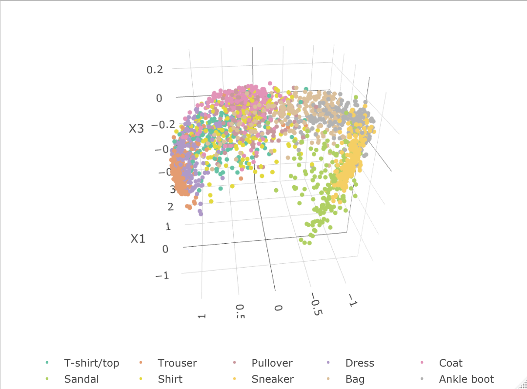


As indicated by the Fashion-MNIST factorization results, both our EFM and the t-SNE methods indicate great separability on the 10 classes with some mistakes on pullover, shirt and coat, which are actually similar classes when we look at the image representation. The NMF performs the worst, utilizing only two dimensions to separate the 10 different classes. Without the stochastic optimization and regularization, the DMF performs no better than our EFM on the testing samples, potentially due to overfitting.
4.3.2. ORL face dataset
To illustrate that our EFM method also provides reasonable uncertainty quantification, we also conducted experiments on the ORL face dataset (Zhu et al., 2019), which contains 40 subjects with pictures taken under 10 different conditions. Each picture is in a 64x64 dimensional space, a high pixel resolution for restoration. To add uncertainty to the image restoration, we cropped part of the face images by setting pixel values to 0. For example, in Figure 8 we can see that the mouth of a person is covered with a white background.

Similar to eigen-face decomposition, we adopt for factorization since we expect to find 40 individual face eigen-vectors and one “average face”. We fit EFM with negative binomial and estimated by using the moment estimator. For comparison, we also conducted eigen-face restoration with rank 40 after centering the “average face”. The result is summarized in Figure 9.
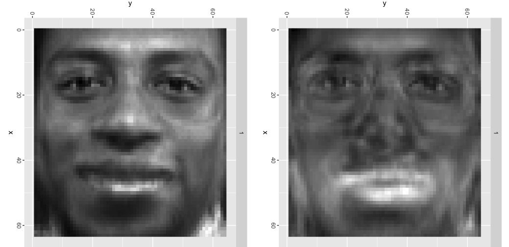
Our EFM not only restores the faces much more accurately compared to eigen-face, but also quantifies the uncertainty in the image restoration. With Laplacian approximation, we compute the MAP estimator of and and simulate the latent variable accordingly. The simulated can then be combined with to provide simulated human faces. As it is shown in Figure 10, the uncertainty due to the crop of the image is correctly identified after centering the simulated faces, which demonstrates different mouth characteristics.

4.4. Network analysis
Another interesting application of our weighted EFM is on social network analysis, where interest often lies in summarizing a large adjacency matrix using lower-dimensional representations named “node embeddings”. Recently, emerging interests has been directed to node embedding inference based upon multiple networks. These multiple networks are formally observed as multiple interaction graphs, , which consists of multiple edge relationships, , for the same sets of vertices . This emerging field of research is named as multi-layer or multiplex network analysis (Kivelä et al., 2014). Denoting the number of vertices as , multiplex network inference starts by transforming these multiple graphs into adjacency matrices of same dimension . Factorization and joint inference on these constructed have been shown to provide better node embeddings with potential applications to community detection and link prediction (Wang et al., 2019; Jones and Rubin-Delanchy, 2020).
One method to enable the joint inference on adjacency matrices is to effectively combine into a single adjacency matrix . Draves (2022, Chapter 2) provides a comprehensive introduction to various aggregation techniques. To briefly summarize some of the relevant aggregation techniques used in this section, there are
-
•
Average Adjacency Spectral Embedding (AASE; Tang et al., 2018) which simply averages the adjacency matrix through
(33) -
•
Unfolded Adjacency Spectral Embedding (UASE) that concatenates the adjacency matrices column-wisely
(34) -
•
Omnibus Embedding (OE) by constructing pair-wisely the following adjacency matrix:
(35)
With and the -dimensional Stiefel manifold of order , we can conduct SVD for the asymmetric from UASE and eigen-decomposition for the symmetric from ASE and OE:
| (36) | ||||
The node embeddings can then be defined as with dimension , where we only take the first entries in the eigenvectors for the Omnibus embedding(Levin et al., 2017).
However, one obvious shortcoming of these aggregations is that the factorization implicitly assumes an equal contribution from each of the layers. In reality, we know that each layer of the network is at least different according to different levels of sparsity. Treating equally the interactions in a dense graph and the interactions in a sparse graph is problematic by over-emphasizing the interactions on the dense graphs. Additionally for the temporal network that consists of the edge relationships of same vertices across different time steps, it intuitively makes more sense if we apply higher weights to the more recent adjacency matrices compared to an equal aggregation on these edge relationships since these recent adjacency matrices should be more informative for the prediction of future interactions.
Naturally one immediate improvement to an equal aggregation of those individual networks is to apply different weights in the factor inference. The EFM provides a solution to this aggregation technique by allowing entry-wise and layer-wise weights to the aggregated interaction. With this flexibility on heuristic weight specification, we demonstrate that we can factorize to obtain improved embedding results for multiplex network analysis.
We thus explore our EFM inference on the AUCS dataset (Dickison et al., 2016).The dataset records interactions among employees at the Department of Computer Science at Aarhus University. As we confirmed with the author, among those 61 employees, there are 55 employees with labels from one of the eight research groups. There are 6 employees that do not belong to any of the eight research groups. The research group labels of those 55 employees can thus be treated as known community structure to validate the effectiveness of community inference.
For the whole community, interactions are recorded according to five different online and offline relationships, whose adjacency matrices can be represented with the following plot:

As we observe from the interaction network data, the co-author network is definitely sparser when compared to other layers of the network. By following the heuristic introduced in the beginning of this section, we propose to weight each interaction of different layer of the network according to the sparsity of the layer. Specifically, with denoted as the largest eigenvalue of adjacency matrix , we
-
•
weight all the diagonal terms with value 0 since the zero interaction of a node with respect to itself does not necessarily contain any information.
-
•
weight each of the interaction according to to ensure that each matrix has its largest eigenvalue equal to 1.
-
•
weight all the remaining zero interactions as the minimal value of the non-zero terms in the weight matrix to reduce the bias effect towards zero of no interactions across all networks.
The weights are then defined as:
| (37) |
Finally, for the aggregated adjacency matrix we assign value 1 to whenever and interact in at least one layer, that is, .
With weight and adjacency matrix definition in Eq (37), we then apply a binomial EFM with logit link to obtain three dimensional nodes embedding. We can then visualize those factorized embedding according the separability of the known research group community labels. For a comparison to the embedding techniques, SVD or eigen-decomposition are also conducted on their corresponding aggregated adjacency matrices to obtain their corresponding nodes embedding defined in Eq (36). The visualization comparison on those factorized embedding is provided below:


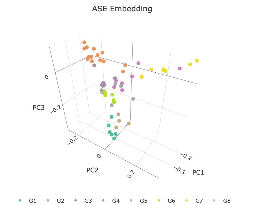
As we can see from Figure 12 the weighted EFM separated more research groups as it is compared to a naive SVD on any of the embedded graphs. The classification result is also consistent with the existing literature (Magnani et al., 2021) who have claimed that there are five major research groups identified by the publisher of the dataset.
5. Conclusion
We propose two classes of flexible, robust, and efficient optimization algorithms for exponential family factor modeling. We start by formally addressing identifiability issues and, in effect, generalizing the singular value decomposition to deviance losses, which should yield more representative results for a broader range of real-world datasets. We address the main computational hurdle, integrating out latent factors, by proposing robust approximation schemes based on EM and SGD optimization. The optimization algorithm improves the simulated likelihood estimation (SML) by eliminating the asymptotic estimation bias with moderate simulation sample size . We provide an efficient R implementation to our proposed optimization algorithm. Additionally, utilizing the SGD optimization, our EFM generalizes better than alternative factorization models such as DMF. Both the simulation studies and empirical studies provide compelling evidence to these advantages.
References
- Ford et al. [1986] J. Kevin Ford, Robert C. MacCallum, and Marianne Tait. The application of exploratory factor analysis in applied psychology: A critical review and analysis. Personnel Psychology, 1986.
- Prince et al. [2008] Simon J D Prince, James H Elder, Jonathan Warrell, and Fatima M Felisberti. Tied factor analysis for face recognition across large pose differences. IEEE Transactions on Pattern Analysis and Machine Intelligence, 2008.
- Fama and French [2015] Eugene F Fama and Kenneth R. French. A five-factor asset pricing model. Journal of Financial Economics, 2015.
- Xu et al. [2021] Tianchen Xu, Ryan T., and Demmer Gen Li. Zero-inflated poisson factor model with application to microbiome read counts. Biometrics, 2021.
- Basilevsky [1994] Alexander Basilevsky. Statistical factor analysis and related methods. Wiley Series in Probability and Mathematical Statistics, 1994.
- Wedel and Kamakura [2001] Michel Wedel and Wagner A. Kamakura. Factor analysis with (mixed) observed and latent variables in the exponential family. Psychometrika, 66:513–30, 2001.
- Wedel et al. [2003] Michel Wedel, Ulf Bo Ckenholt, and Wagner A. Kamakurac. Factor models for multivariate count data. Journal of Multivariate Analysis, 2003.
- Bartholomew et al. [2011] David J Bartholomew, Martin Knott, and Irini Moustaki. Latent variable models and factor analysis: A unified approach. John Wiley & Sons, 2011.
- Tipping and Bishop [1998] Michael E. Tipping and Christopher M. Bishop. Probabilistic principal component analysis. Journal of the Royal Statistical Society, Series B, 1998.
- Anderson [1963] Theodore Wilbur Anderson. The use of factor analysis in the statistical analysis of multiple time series. Psychometrika, 1963.
- Wang and Carvalho [2023] Liang Wang and Luis Carvalho. Deviance matrix factorization. Electronic Journal of Statistics, 17(2):3762–3810, 2023.
- Fan et al. [2008] Jianqing Fan, Yingying Fan, and Jinchi Lv. High dimensional covariance matrix estimation using a factor model. Journal of Econometrics, 147(1):186–197, 2008.
- Borenstein et al. [2010] Michael Borenstein, Larry V Hedges, Julian PT Higgins, and Hannah R Rothstein. A basic introduction to fixed-effect and random-effects models for meta-analysis. Research synthesis methods, 1(2):97–111, 2010.
- Carter and Kohn [1996] Chris K Carter and Robert Kohn. Markov chain monte carlo in conditionally gaussian state space models. Biometrika, 83(3):589–601, 1996.
- Shapiro [1985] Alexander Shapiro. Identifiability of factor analysis: Some results and open problems. Linear Algebra and its Applications, 70:1–7, 1985.
- Kaiser [1958] Henry F Kaiser. The varimax criterion for analytic rotation in factor analysis. Psychometrika, 23(3):187–200, 1958.
- Gribonval and Schnass [2010] Rémi Gribonval and Karin Schnass. Dictionary identification—sparse matrix-factorization via -minimization. IEEE Transactions on Information Theory, 56(7):3523–3539, 2010.
- Lee and Choi [1999] Daniel D. Lee and Seung Hoe Choi. Learning the parts of objects by nonnegative matrix factorization. Nature, 401, 1999.
- Li et al. [2010] Zhao Li, Xindong Wu, and Hong Peng. Nonnegative matrix factorization on orthogonal subspace. Pattern Recognition Letters, 31(9):905–911, 2010.
- Ma and Fu [2012] Yunqian Ma and Yun Fu. Manifold learning theory and applications, volume 434. CRC press Boca Raton, 2012.
- Jeffrey Pennington and Manning [2014] Richard Socher Jeffrey Pennington and Christopher Manning. Glove: Global vectors for word representation. Proceedings of the 2014 Conference on Empirical Methods in Natural Language Processing (EMNLP), pages 1532–1543, 2014.
- Kalayeh et al. [2014] Mahdi M Kalayeh, Haroon Idrees, and Mubarak Shah. Nmf-knn: Image annotation using weighted multi-view non-negative matrix factorization. In Proceedings of the IEEE conference on computer vision and pattern recognition, pages 184–191, 2014.
- Davenport et al. [2014] Mark A Davenport, Yaniv Plan, Ewout Van Den Berg, and Mary Wootters. 1-bit matrix completion. Information and Inference: A Journal of the IMA, 3(3):189–223, 2014.
- Reimann et al. [2002] Clemens Reimann, Peter Filzmoser, and Robert G Garrett. Factor analysis applied to regional geochemical data: problems and possibilities. Applied geochemistry, 17(3):185–206, 2002.
- Gopalan et al. [2015] Prem Gopalan, Jake M. Hofman, and David M. Blei. Scalable recommendation with hierarchical poisson factorization. Proceedings of the Thirty-First Conference on Uncertainty in Artificial Intelligence, 2015.
- Ruan and Di [2024] Kangrui Ruan and Xuan Di. Infostgcan: An information-maximizing spatial-temporal graph convolutional attention network for heterogeneous human trajectory prediction. Computers, 13(6), 2024. URL https://www.mdpi.com/2073-431X/13/6/151.
- Rue et al. [2009] Havard Rue, Sara Martino, and Nicolas Chopin. Approximate bayesian inference for latent gaussian models by using integrated nested laplace approximations. Journal of the Royal Statistical Society, Series B, 2009.
- Wu and Zhang [2003] Ningning Wu and Jing Zhang. Factor analysis based anomaly detection. IEEE Systems, Man and Cybernetics SocietyInformation Assurance Workshop, 2003.
- Lee [1995] Lung-fei Lee. Asymptotic bias in simulated maximum likelihood estimation of discrete choice models. Econometric Theory, 11:437–83, 1995.
- Li et al. [2024] Zhenglin Li, Haibei Zhu, Houze Liu, Jintong Song, and Qishuo Cheng. Comprehensive evaluation of mal-api-2019 dataset by machine learning in malware detection. arXiv preprint arXiv:2403.02232, 2024.
- Kitagawa [1987] Genshiro Kitagawa. Non-gaussian state—space modeling of nonstationary time series. Journal of the American statistical association, 82(400):1032–1041, 1987.
- Levy and Goldberg [2014] Omer Levy and Yoav Goldberg. Neural word embedding as implicit matrix factorization. Advances in neural information processing systems, 27, 2014.
- Mikolov et al. [2013] Tomas Mikolov, Kai Chen, Greg Corrado, and Jeffrey Dean. Efficient estimation of word representations in vector space. arXiv preprint arXiv:1301.3781, 2013.
- Hoff et al. [2002] Peter D Hoff, Adrian E Raftery, and Mark S Handcock. Latent space approaches to social network analysis. Journal of the american Statistical association, 97(460):1090–1098, 2002.
- Young and Scheinerman [2007] Stephen J Young and Edward R Scheinerman. Random dot product graph models for social networks. In Algorithms and Models for the Web-Graph: 5th International Workshop, WAW 2007, San Diego, CA, USA, December 11-12, 2007. Proceedings 5, pages 138–149. Springer, 2007.
- Wedderburn [1974] Robert WM Wedderburn. Quasi-likelihood functions, generalized linear models, and the Gauss-Newton method. Biometrika, 61(3):439–447, 1974.
- Xia [2020] Weixuan Xia. The average of a negative-binomial lévy process and a class of lerch distributions. Communications in Statistics-Theory and Methods, 49(4):1008–1024, 2020.
- Nelder and Pregibon [1987] John A Nelder and Daryl Pregibon. An extended quasi-likelihood function. Biometrika, 74(2):221–232, 1987.
- Dempster et al. [1977a] Arthur P Dempster, Nan M Laird, and Donald B Rubin. Maximum likelihood from incomplete data via the EM algorithm. Journal of the Royal Statistical Society: Series B (Methodological), 39(1):1–22, 1977a.
- Golub and Welsch [1969] Gene H Golub and John H Welsch. Calculation of Gauss quadrature rules. Mathematics of computation, 23(106):221–230, 1969.
- Fan et al. [2020] Jianqing Fan, Jianhua Guo, and Shurong Zheng. Estimating number of factors by adjusted eigenvalues thresholding. Journal of the American Statistical Association, 2020.
- Robbins and Monro [1951] Herbert Robbins and Sutton Monro. A stochastic approximation method. The annals of mathematical statistics, pages 400–407, 1951.
- Bertsekas [1999] Dimitri P. Bertsekas. Nonlinear programming: 2nd edition. Athena Scientific, 1999.
- Duchi et al. [2011] John Duchi, Elad Hazan, and Yoram Singer. Adaptive subgradient methods for online learning and stochastic optimization. The Journal of Machine Learning Research, 2011.
- Ieleman and Hinton [2012] T. Ieleman and G Hinton. Neural networks for machine learning. Technical report, 2012.
- Kingma and Ba [2015] Diederik P. Kingma and Jimmy Ba. Adam: A method for stochastic optimization. 3rd International Conference on Learning Representations, ICLR 2015, 2015.
- Tierney and Kadane [1986] Luke Tierney and Joseph B Kadane. Accurate approximations for posterior moments and marginal densities. Journal of the american statistical association, 81(393):82–86, 1986.
- Xia and Zhang [2023] Weixuan Xia and Yuyang Zhang. On the absolute-value integral of a brownian motion with drift: Exact and asymptotic formulae. arXiv preprint arXiv:2312.04172, 2023.
- Tierney et al. [1989] Luke Tierney, Robert E Kass, and Joseph B Kadane. Fully exponential laplace approximations to expectations and variances of nonpositive functions. Journal of the american statistical association, 84(407):710–716, 1989.
- Dempster et al. [1977b] A. P. Dempster, N. M. Laird, and D. B. Rubin. Maximum likelihood from incomplete data via the em algorithm. Journal of the Royal Statistical Society: Series B (Methodological), 39:1–22, 1977b.
- Jank and Booth [2003] Wolfgang Jank and James Booth. Efficiency of monte carlo em and simulated maximum likelihood in two-stage hierarchical models. Journal of Computational and Graphical Statistics, 12:214–29, 2003.
- Caffo et al. [2005] Brian S Caffo, Wolfgang Jank, and Galin L Jones. Ascent-based monte carlo expectation–maximization. Journal of the Royal Statistical Society: Series B (Statistical Methodology), 67(2):235–251, 2005.
- Jank [2006] Wolfgang Jank. Implementing and diagnosing the stochastic approximation em algorithm. Journal of Computational and Graphical Statistics, 15:803–29, 2006.
- Yao et al. [2007] Yuan Yao, Lorenzo Rosasco, and Andrea Caponnetto. On early stopping in gradient descent learning. Constructive Approximation, 26(2):289–315, 2007.
- Pishchik [2023] Evgenii Pishchik. Trainable activations for image classification. 2023.
- Xiao et al. [2017] Han Xiao, Kashif Rasul, and Roland Vollgraf. Fashion-mnist: a novel image dataset for benchmarking machine learning algorithms, 2017.
- Zhu et al. [2019] Pengfei Zhu, Binyuan Hui, Changqing Zhang, Dawei Du, Longyin Wen, and Qinghua Hu. Multi-view deep subspace clustering networks. arXiv preprint arXiv:1908.01978, 2019.
- Kivelä et al. [2014] Mikko Kivelä, Alex Arenas, Marc Barthelemy, James P Gleeson, Yamir Moreno, and Mason A Porter. Multilayer networks. Journal of complex networks, 2(3):203–271, 2014.
- Wang et al. [2019] Shangsi Wang, Jesús Arroyo, Joshua T Vogelstein, and Carey E Priebe. Joint embedding of graphs. IEEE transactions on pattern analysis and machine intelligence, 43(4):1324–1336, 2019.
- Jones and Rubin-Delanchy [2020] Andrew Jones and Patrick Rubin-Delanchy. The multilayer random dot product graph. arXiv preprint arXiv:2007.10455, 2020.
- Draves [2022] Benjamin Draves. Joint spectral embeddings of random dot product graphs. PhD thesis, Boston University, 2022.
- Tang et al. [2018] Runze Tang, Michael Ketcha, Alexandra Badea, Evan D Calabrese, Daniel S Margulies, Joshua T Vogelstein, Carey E Priebe, and Daniel L Sussman. Connectome smoothing via low-rank approximations. IEEE transactions on medical imaging, 38(6):1446–1456, 2018.
- Levin et al. [2017] Keith Levin, Avanti Athreya, Minh Tang, Vince Lyzinski, Youngser Park, and Carey E Priebe. A central limit theorem for an omnibus embedding of multiple random graphs and implications for multiscale network inference. arXiv preprint arXiv:1705.09355, 2017.
- Dickison et al. [2016] Mark E Dickison, Matteo Magnani, and Luca Rossi. Multilayer social networks. Cambridge University Press, 2016.
- Magnani et al. [2021] Matteo Magnani, Luca Rossi, and Davide Vega. Analysis of multiplex social networks with r. Journal of Statistical Software, 98:1–30, 2021.