Compression of M^♮-convex Functions — Flag Matroids and Valuated Permutohedra

A function $f:2^{E}\to\mathbb{R}$ is called a submodular function if it satisfies

We assume that $f(\emptyset)=0$ for any set function $f:2^{E}\to\mathbb{R}$ in the sequel. A negative of a submodular function is called a supermodular function. (Also see [4, 9].)

For a submodular function $f:2^{E}\to\mathbb{R}$ define

which is called the submodular polyhedron associated with submodular function $f$. Also define

which is called the base polyhedron associated with submodular function $f$. As is well known (see [9]), the base polyhedron ${\rm B}(f)$ is always nonempty (and is a face of ${\rm P}(f)$).

For a supermodular function $g:2^{E}\to\mathbb{R}$ we define in a dual manner the supermodular polyhedron

and the base polyhedron

For a submodular function $f:2^{E}\to\mathbb{R}$ define a supermodular function $f^{\#}:2^{E}\to\mathbb{R}$ by

which is called the dual supermodular function of $f$. Then we have ${\rm B}(f)={\rm B}(f^{\#})$. For more details about submodular/supermodular functions and associated polyhedra see [9, Chapter II], where submodular/supermodular functions defined on distributive lattices ${\mathcal{D}}\subseteq 2^{E}$ are also investigated and their base polyhedra are unbounded unless $\mathcal{D}=2^{E}$.

Define $Q_{\mathbb{Z}}=Q\cap\mathbb{Z}^{E}$ for any set $Q\subseteq\mathbb{R}^{E}$. Also denote by ${\rm Conv}(Q)$ the convex hull of $Q$ in $\mathbb{R}^{E}$. When ${\rm Conv}(Q_{\mathbb{Z}})=Q$, we identify $Q$ with $Q_{\mathbb{Z}}$.

When a submodular function $f:2^{E}\to\mathbb{R}$ is integer-valued, its submodular polyhedron and base polyhedron are integral (i.e., every vertex of the polyhedra is an integral vector). Moreover, we have

Most of the following arguments are valid even if we regard $\mathbb{Z}$ in place of $\mathbb{R}$ as the underlying totally ordered additive group. When $f$ is integer-valued, we call ${\rm P}(f)_{\mathbb{Z}}$ and ${\rm B}(f)_{\mathbb{Z}}$ the submodular polyhedron and the base polyhedron, respectively, associated with $f$ as well. (This is the approach taken in [9], indeed.)

For a submodular function $f:2^{E}\to\mathbb{R}$ and a nonempty proper subset $A$ of $E$ define functions $f^{A}:2^{A}\to\mathbb{R}$ and $f_{A}:2^{E\setminus A}\to\mathbb{R}$ by

We also define $f^{E}=f_{\emptyset}=f$. We call $f^{A}$ the restriction of $f$ on $A$ and $f_{A}$ the contraction of $f$ by $A$. Similarly we define the restriction and contraction for supermodular functions.

For a permutation $\pi:[n]\to[n]$ we identify $\pi$ with the permutation vector $(\pi(1),\cdots,\pi(n))$ in $\mathbb{Z}^{n}$, which we denote by $v_{\pi}$ (or simply by $\pi$ when there is no possibility of confusion). Suppose that an integer-valued submodular function $f:2^{E}\to\mathbb{Z}$ is given by $f(X)=\sum_{i=1}^{|X|}(n-i+1)$ for all $X\subseteq E=[n]$. Then the base polyhedron ${\rm B}(f)$ has the $n!$ extreme points, each being a permutation vector identified with a permutation of $[n]$, which is called the permutohedron (or permutahedron) in $\mathbb{R}^{E}$.

For any permutation $\pi$ of $[n]$ we have a unique complete flag

such that for each $i\in[n]$ $F_{i}$ is the set of the first $i$ elements of $(\pi(1),\cdots,\pi(n))$, i.e.,

1. 1.

   $|F_{i}|=i$ for each $i=1,\cdots,n$ and

2. 2.

   $\displaystyle{\sum_{i=1}^{n}\chi_{F_{i}}=v_{\pi}}$, where $\chi_{F_{i}}$ is the characteristic vector of a set $F_{i}\subseteq[n]$.

Denote the flag $\mathcal{F}$ in (2.9) by $\mathcal{F}^{\pi}:F^{\pi}_{1}\subset\cdots\subset F^{\pi}_{n}$.

Let us consider a polyhedron $P$ satisfying the following two:

• (P1)

  $P$ is the convex hull of a set of some permutation vectors.

• (P2)

  $P$ is a base polyhedron.

We call such a polyhedron $P$ a sub-permutohedron.³³3 We may call the sub-permutohedron a permutohedron, and an ordinary permutohedron a complete permutohedron, but we resist the temptation. A sub-permutohedron is precisely the Coxeter matroid polytope associated with a flag matroid of complete flag (see [2] and the discussions to be made in Section 5). A recent interesting appearance of a sub-permutohedron is from the theory of Bruhat order ([1]), due to Tsukerman and Williams [19], that every Bruhat interval polytope is a sub-permutohedron.

Suppose that a submodular function $f:2^{E}\to\mathbb{R}$ and a supermodular function $g:2^{E}\to\mathbb{R}$ with $f(\emptyset)=g(\emptyset)=0$ satisfy the following inequalities

Then the polyhedron

is called a generalized polymatroid ([6, 10]). There exists a one-to-one correspondence between base polyhedra and generalized polymatroids up to translation along a coordinate axis as follows (see [9, Figure 3.7]).

When a generalized polymatroid is a convex hull of $\{0,1\}$-valued points (vertices), then it is called a generalized-matroid polytope, which can be identified with the family ${\mathcal{G}}$ of subsets $X\subseteq E$ such that $\chi_{X}$ are vertices of the generalized-matroid polytope. The family $\mathcal{G}$ is called a generalized matroid (see [7]).

An ordered pair $(f_{1},f_{2})$ of submodular functions $f_{i}:2^{E}\to\mathbb{R}$ $(i=1,2)$ is called a weak map if we have

Moreover, the ordered pair $(f_{1},f_{2})$ is called a strong map if we have

i.e., every ordered pair $((f_{1})_{X},(f_{2})_{X})$ of contractions of $f_{1}$ and $f_{2}$ by $X\subset E$ is a weak map. The concept of strong map was originally considered for matroids (see [17, 18, 20]), and we adopt it to any submodular functions (or submodular systems).

We also have the following theorem.

A sequence of submodular functions $f_{1},\cdots,f_{p}:2^{E}\to\mathbb{R}$ is called a strong map sequence if for each $i=1,\cdots,$ $p$$-$$1$ the pair $(f_{i+1},f_{i})$ is a strong map. It follows from Theorem 2.2 that

• (F1)

  Given a strong map sequence $f_{1},\cdots,f_{p}:2^{E}\to\mathbb{R}$, we have a sequence of generalized polymatroids ${\rm P}(f_{i+1},(f_{i})^{\#})$ for $i=1,\cdots,p-1$.

We also have the following.

• (F2)

  For a generalized polymatroid ${\rm P}(f,g)$ and $\alpha\in\mathbb{R}$ such that $g(E)\leq\alpha\leq f(E)$ the intersection of ${\rm P}(f,g)$ and the hyperplane $x(E)=\alpha$ is a base polyhedron (we call such a base polyhedron a section of ${\rm P}(f,g)$ and denote it by ${\rm P}(f,g)_{(\alpha)}$). When ${\rm P}(f,g)$ is integral and $\alpha$ is an integer, the section ${\rm P}(f,g)_{(\alpha)}$ is integral. Moreover, letting ${\rm B}(f^{\prime})$ be a section of ${\rm P}(f,g)$ with a submodular function $f^{\prime}$, we have a strong map sequence $g^{\#},f^{\prime},f$, i.e., ${\rm P}(f^{\prime},g)$ and ${\rm P}(f,(f^{\prime})^{\#})$ are generalized polymatroids.

A strong map sequence $f_{1},\cdots,f_{p}:2^{E}\to\mathbb{Z}$ with $f_{i}$ $(i=1,\cdots,p)$ being matroid rank functions is called a flag matroid (see [2]).

Let $f:\mathbb{R}^{E}\to\mathbb{R}\cup\{+\infty\}$ be a polyhedral convex function such that

1. 1.

   its effective domain, ${\rm dom}f\equiv\{x\in\mathbb{R}^{E}\mid f(x)<+\infty\}$, is a generalized polymatroid (hence nonempty) and

2. 2.

   every linearity domain of $f$ is a generalized polymatroid,

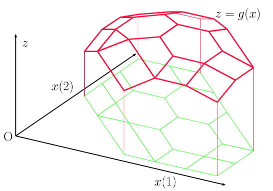
where a linearity domain (or affinity domain) of $f$ is ${\rm Arg}\min(f-h)$ for a linear function $h(x)=\langle z,x\rangle(\equiv\sum_{e\in E}z(e)x(e))$ with some $z\in(\mathbb{R}^{E})^{*}$. Then $f$ is called an M^♮-convex function⁴⁴4Here we employ another equivalent definition of M^♮-convexity, instead of the original definition by means of the exchange axiom introduced by Murota and Shioura [16, 13]., which is due to Murota and Shioura [16, 13] (also see [9, Section 17]). The negative of an M^♮-convex function is called an M^♮-concave function (see Figure 1).

When ${\rm dom}f$ of an M^♮-convex function $f$ is a base polyhedron, $f$ is called an M-convex function (see [13]).⁵⁵5 M-convex functions were introduced earlier than M^♮-convex functions by Murota (see [12, 13]). There is a one-to-one correspondence between M-convex functions and M^♮-convex convex functions because of Theorem 2.1. Any concept related to M-/M^♮-concave functions is defined in a natural way from that defined for M-/M^♮-convex functions.

Now let $f:\mathbb{R}^{E}\to\mathbb{R}\cup\{+\infty\}$ be an M^♮-convex function satisfying the following (a) and (b):

• (a)

  The effective domain of $f$ is an integral generalized polymatroid.

• (b)

  Every linearity domain of $f$ is also an integral generalized polymatroid.

Such an M^♮-convex function $f$ can be identified with $f$ being restricted on the integer lattice $\mathbb{Z}^{E}$. So we can consider an M^♮-convex function $f:\mathbb{Z}^{E}\to\mathbb{R}\cup\{+\infty\}$. An integer-valued M-concave function $g:\mathbb{Z}^{E}\to\mathbb{Z}\cup\{+\infty\}$ with its effective domain being a matroid base polytope coincides with a valuated matroid due to Dress and Wenzel [3]. Also, if an M^♮-convex function $f:\mathbb{Z}^{E}\to\mathbb{R}\cup\{+\infty\}$ has an effective domain ${\rm dom}(f)$ whose convex hull ${\rm Conv}({\rm dom}(f))$ is a permutohedron, we call $f$ a valuated permutohedron.

For any M^♮-convex function $f:\mathbb{R}^{E}\to\mathbb{R}\cup\{+\infty\}$ define the Legendre-Fenchel transform (or convex conjugate) of $f$ by

where $\langle y,x\rangle=\sum_{e\in E}y(e)x(e)$. The function $f^{\bullet}$ is called an L^♮-convex function ([13]), which is equivalent to submodular integrally convex function due to Favati and Tardella [5]. The original $f$ is recovered from $f^{\bullet}$ by taking another Legendre-Fenchel transform as follows.

(See [13, 14].) Hence there exists a one-to-one correspondence between M^♮-convex functions and L^♮-convex functions. Furthermore, Murota [13] showed the integrality property that (2.17) and (2.18) with $\mathbb{R}$ being replaced by $\mathbb{Z}$ hold for any M^♮-convex function $f:\mathbb{Z}^{E}\to\mathbb{Z}\cup\{+\infty\}$. When $f$ is an M-convex function, its Legendre-Fenchel transform is what is called an L-convex function ([13]).

For any $x\in\mathbb{R}^{E}$ the subdifferential of $f$ at $x$, denoted by $\partial f(x)$, is defined by

The subdifferential of $f^{\bullet}$ is defined similarly as

Then we have the following.

For more details about M-/M^♮-convex functions and L-/L^♮-convex functions see [13, 14] and [9, Chapter VII].

For the compression $\hat{f}$ of $f$ and for any $w\in(\mathbb{R}^{E})^{*}$ let us define $D(\hat{f},w)\subseteq\mathbb{Z}^{E}$ and $D(f_{(\alpha)},w)\subseteq\mathbb{Z}^{E}$ $(\alpha\in I_{f})$ by

where recall (3.2) for the definition of $I_{f}$. We call $D(\hat{f},w)$ and $D(f_{(\alpha)},w)$ $(\alpha\in I_{f})$ linearity domains of $\hat{f}$ and $f_{(\alpha)}$ $(\alpha\in I_{f})$, respectively, associated with $w$. We see from Lemma 2.3 that for every $x\in\mathbb{Z}^{E}$ we have

This means that the linearity domains of $\hat{f}$ are exactly the subdifferentials of $\hat{f}^{\bullet}$.

Let $\mathbb{S}$ be the collection of all maximal linearity domains of $\hat{f}$ (or maximal subdifferentials of $\hat{f}^{\bullet}$). Then $\mathbb{S}$ gives a polyhedral division of ${\rm dom}(\hat{f})$ into generalized polymatroids. Since ${\rm dom}(f)$ is full-dimensional, the dimension of ${\rm dom}(\hat{f})$ is equal to $|E|-1(=n-1)$.

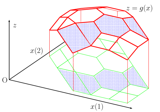
For each maximal linearity domain $S\in\mathbb{S}$ of $\hat{f}$ let $w$ be a vector in $(\mathbb{R}^{E})^{*}$ such that $S=\partial\hat{f}^{\bullet}(w)$ and put ${D}(\alpha,S)=D({f}_{(\alpha)},w)$ $(\alpha\in I_{f})$, which are independent of the choice of $w$ satisfying $S=\partial\hat{f}^{\bullet}(w)$. Define ${D}(S)=\bigcup\{{D}(\alpha,S)\mid\alpha\in I_{f}\}$ and let $f^{{D}(S)}$ be the restriction of $f$ on ${D}(S)$. Then we call $f^{{D}(S)}=(f_{(\alpha)}^{{D}(\alpha,S)}\mid\alpha\in I_{f})$ a strip of $f$ associated with $S\in\mathbb{S}$, where $f_{(\alpha)}^{{D}(\alpha,S)}$ is the restriction of $f_{(\alpha)}$ on ${D}(\alpha,S)$. (See Figure 2 for an example of a strip of an M^♮-concave function.) The collection of the strips $f^{{D}(S)}$ for all $S\in\mathbb{S}$ is called the strip decomposition of $f$.

For any strip $f^{{D}(S)}=(f_{(\alpha)}^{{D}(\alpha,S)}\mid\alpha\in I_{f})$ of an M^♮-convex function $f$ associated with $S\in\mathbb{S}$ let $w$ be a vector in $(\mathbb{R}^{E})^{*}$ such that $S=\partial\hat{f}^{\bullet}(w)$. Then consider a parametric optimization problem ${\bf P}(\lambda)$ with a parameter $\lambda\in\mathbb{R}$ described as follows.

where ${\bf 1}=\chi_{E}$ is the $n$-dimensional vector of all ones. We then have the following theorem.

Here it should be noted that values $\lambda_{i}$ $(i=1,\cdots,p)$ depend on the choice of $w\in S$, while the vectors $w+\lambda_{i}{\bf 1}$ $(i=1,\cdots,p)$ are uniquely determined by $f$ and $S\in\mathbb{S}$, because of the assumptions that ${\rm dom}(f)$ is full-dimensional and $S\in\mathbb{S}$ is a maximal linearity domain of $\hat{f}$.

For a valuated generalized matroid $f:2^{E}\to\mathbb{Z}$ the compression $\hat{f}$ of $f$ given by (3.3) becomes

where ${E\choose\alpha}=\{X\subseteq E\mid|X|=\alpha\}$ for $\alpha\in[n]$, and we define $\hat{f}(x)=+\infty$ if the minimum on the right-hand side does not exist for $x\in\mathbb{Z}^{E}$. Then the effective domain of the compression $\hat{f}$ given by (3.6) is expressed by the following Minkowski sum:

Recall that $E=[n]$.

For every $S\in\mathbb{S}$ we have the strip $f^{{D}(S)}=(f_{(\alpha)}^{{D}(\alpha,S)}\mid\alpha=0,1,\cdots,n)$ of $f$ associated with $S\in\mathbb{S}$, which is characterized as follows. We identify $\chi_{X}$ with $X$ for any $X\subseteq[n]$.

We call the flag matroid $(\rho_{\alpha}^{S}\mid\alpha=0,1,\cdots,n)$ the flag matroid associated with a strip $S\in\mathbb{S}$ (or a flag-matroid strip) of the valuated generalized matroid $f$. We see from Theorems 5.1 and 5.2 the following.

Every valuated generalized matroid is regarded as a valuated permutohedron endowed with valuated flag-matroid strips, one for each maximal linearity domain of it.

References

- [1] A. Björner and F. Brenti: Combinatorics of Coxeter Groups (Graduate Texts in Mathematics 231), Springer, 2005.
- [2] A. V. Borovik, I. M. Gelfand and N. White: Coxeter Matroids (Progress in Mathematics, Vol. 216) (Birkhäuser, Boston, 2003).
- [3] A. W. M. Dress and W. Wenzel: Valuated matroids. Advances in Mathematics 93 (1992) 214–250.
- [4] J. Edmonds: Submodular functions, matroids, and certain polyhedra. Proceedings of the Calgary International Conference on Combinatorial Structures and Their Applications (R. Guy, H. Hanani, N. Sauer and J. Schönheim, eds., Gordon and Breach, New York, 1970), pp. 69–87; also in: Combinatorial Optimization—Eureka, You Shrink! (M. Jünger, G. Reinelt and G. Rinaldi, eds., Lecture Notes in Computer Science 2570, Springer, Berlin, 2003), pp. 11–26.
- [5] P. Favati and F. Tardella: Convexity in nonlinear integer programming. Ricerca Operativa 53 (1990) 3–44.
- [6] A. Frank: Generalized polymatroids. Proceedings of the Sixth Hungarian Combinatorial Colloquium (Eger, 1981); also, Finite and Infinite Sets, I (A. Hajnal, L. Lovász and V. T. Sós, eds., Colloquia Mathematica Societatis János Bolyai 37, North-Holland, Amsterdam, 1984), pp. 285–294.
- [7] A. Frank and É. Tardos: Generalized polymatroids and submodular flows. Mathematical Programming 42 (1988) 489–563.
- [8] S. Fujishige: A note on Frank’s generalized polymatroids. Discrete Applied Mathematics 7 (1984) 105–109.
- [9] S. Fujishige: Submodular Functions and Optimization (North-Holland, 1991), Second Edition (Elsevier, 2005).
- [10] R. Hassin: Minimum cost flow with set-constraints. Networks 12 (1982) 1–21.
- [11] K. Murota: Matroid valuation on independent sets. Journal of Combinatorial Theory 69B (1997) 59–78.
- [12] K. Murota: Discrete convex analysis. Mathematical Programming, Ser. A 83 (1998) 313–371.
- [13] K. Murota: Discrete Convex Analysis (SIAM Monographs on Discrete Mathematics and Applications 10, SIAM, 2003).
- [14] K. Murota: Discrete convex analysis: A tool for economics and game theory, Journal of Mechanism and Institution Design, 1 (2016) 151–273.
-
[15]
K. Murota: A survey of fundamental operations on discrete
convex functions of various kinds. Optimization Methods and Software (to appear)
DOI: 10.1080/10556788.2019.1692345 - [16] K. Murota and A. Shioura: M-convex function on generalized polymatroid. Mathematics of Operations Research 24 (1999) 95–105.
- [17] J. Oxley: Matroid Theory (Oxford University Press, Oxford, 1992).
- [18] A. Schrijver: Combinatorial Optimization—Polyhedra and Efficiency (Springer, Heidelberg, 2003).
- [19] E. Tsukerman and L. Williams: Bruhat interval polytopes. Advances in Mathematics 285 (2015) 766–810.
- [20] D. J. A. Welsh: Matroid Theory (Academic Press, London, 1976).