Compression and Distillation of Data Quadruplets in Non-intrusive Reduced-order Modeling

Umair Zulfiqar [email protected] School of Electronic Information and Electrical Engineering, Yangtze University, Jingzhou, Hubei, 434023, China

Abstract

The data-driven implementation of balanced truncation has been successfully achieved in the literature by approximating the integrals of Gramians using numerical integration. This formulation is non-intrusive, meaning it does not require access to the transfer function or state-space model for constructing reduced-order models. Instead, it relies on samples of the transfer function evaluated along the $j\omega$ -axis or on samples of the impulse response in the time domain. Similarly, the data-driven formulation of iterative rational Krylov algorithm (IRKA) also relies on samples of the transfer function and its derivatives, but unlike balanced truncation, the sampling points are updated iteratively and are not known in advance. If the transfer function is unavailable, IRKA must either pause until new samples are obtained through experiments or estimate new samples from existing data.

This paper introduces a quadrature-free, data-driven approach to balanced truncation for both continuous-time and discrete-time systems. The method non-intrusively constructs reduced-order models using available transfer function samples from the right half of the $s$ -plane. It is highlighted that the proposed data-driven balanced truncation and existing quadrature-based balanced truncation algorithms share a common feature: both compress their respective data quadruplets to derive reduced-order models. Additionally, it is demonstrated that by using different compression strategies, these quadruplets can be utilized to develop three data-driven formulations of the IRKA. These formulations non-intrusively generate near-optimal reduced models using transfer function samples from the $j\omega$ -axis or the right half of the $s$ -plane, or impulse response samples. Notably, these IRKA formulations eliminate the necessity of computing new transfer function samples as IRKA iteratively updates the sampling points. The results are also extended to discrete-time systems. The efficacy of the proposed algorithms is validated through numerical examples, which show that the proposed data-driven approaches perform comparably to their intrusive counterparts.

keywords:

ADI, Balanced truncation, Data-driven,

\mathcal{H}_{2}

-optimal, IRKA, Low-rank, Non-intrusive

^†^†journal: ArXiv.org

1 Introduction

Model order reduction (MOR) comprises system-theoretic methods aimed at constructing simplified models that accurately replicate the input-output behavior of large-scale dynamical systems. By efficiently capturing key dynamical characteristics of the original system, reduced order models (ROMs) are able to approximate its behavior across a broad range of inputs, yet are significantly lower in order. These ROMs are designed to be computationally efficient, making them easier to simulate, manipulate, and control. For further details on various MOR techniques, the readers are referred to [1, 2, 3].

Balanced truncation (BT) [4] is a highly effective and widely used technique for MOR of linear dynamical systems. This method preserves the asymptotic stability of the original system while offering a priori error bounds for the ROM. By discarding states that are difficult to reach and observe, as determined by the relative magnitude of the system’s Hankel singular values, BT ensures that their impact on the system’s input-output behavior is minimal. Consequently, the ROM accurately approximates the original system in simulations or analyses.

The primary computational burden in BT lies in solving large-scale Lyapunov equations to compute the system Gramians. Various approaches, such as those mentioned in the surveys [5, 6], have been developed to efficiently compute these Gramians. These methods rely on the system’s explicit state-space representation, making BT an “intrusive” method. This is in contrast to “non-intrusive” methods, which are data-driven and depend solely on system response data—like transfer function samples or impulse response measurements—without requiring the system’s internal state-space representation [7, 8, 9, 10]. In [11], a non-intrusive BT algorithm based on numerical integration, called Quadrature-BT (QuadBT), is introduced. This algorithm constructs the ROM using transfer function samples at the $j\omega$ -axis of the $s$ -plane or samples of impulse response and its derivatives.

The $\mathcal{H}_{2}$ -optimal MOR problem involves finding a local minimum for the (squared) $\mathcal{H}_{2}$ norm of the error transfer function. One of the key methods for achieving this local optimum is the Iterative Rational Krylov Algorithm (IRKA) [12]. A non-intrusive, data-driven version of IRKA was introduced in [13], based on the interpolatory framework proposed in [7]. This approach requires only transfer function samples and their derivatives to compute the local optimum, making it data-driven and non-intrusive. However, because IRKA is iterative, the sampling points are updated at each iteration and cannot be predetermined. Instead, IRKA identifies the optimal sampling points through successive iterations. If these new samples must be obtained experimentally, the algorithm must pause until the new data is available. This poses practical challenges, as it may be difficult or even impossible to conduct experiments to gather transfer function samples each time the sampling points are updated.

Among the various $\mathcal{H}_{2}$ MOR algorithms, the Pseudo-optimal Rational Krylov (PORK) algorithm is an important suboptimal method [14, 15]. Unlike IRKA, PORK is an iteration-free approach that satisfies a subset of the $\mathcal{H}_{2}$ optimality conditions in a single run. In this paper, PORK plays a significant role in the development of the non-intrusive implementations of both BT and IRKA.

Over the past two decades, the low-rank Alternating-direction Implicit (ADI) method has proven highly effective in reducing the computational cost of BT [16]. It is now one of the most widely used and efficient BT algorithms in the literature [17]. In this paper, we introduce a non-intrusive, data-driven implementation of the low-rank ADI-based BT that constructs the ROM from transfer function samples in the right-half of the $s$ -plane. Unlike QuadBT, this approach does not rely on numerical integration. Additionally, we propose three non-intrusive, data-driven implementations for IRKA, tailored to the type of data available. In cases where transfer function samples along the $j\omega$ axis or impulse response measurements are accessible, we present numerical integration-based algorithms that do not require new transfer function samples as IRKA updates the sampling points. For scenarios where transfer function samples in the right-half of the $s$ -plane are available, we propose a version that does not require numerical integration and new transfer function samples as IRKA updates the sampling points. Additionally, all these data-driven implementations (both BT and IRKA) for continuous-time systems are extended to discrete-time systems in this paper. It is also briefly highlighted that the implementations utilizing transfer function samples in the right half of the $s$ -plane can also be executed using input-output data instead of relying solely on transfer function samples.

The remainder of the paper is structured as follows. Section 2 provides the necessary background on MOR and briefly reviews existing MOR algorithms most relevant to this work. The main contributions of this research begin in Section 3, where a data-driven, non-intrusive implementation of ADI-based low-rank BT is proposed. Section 4 presents three new data-driven implementations of IRKA, tailored to the type of available data. Section 5 introduces two quadrature-based data-driven implementations of IRKA for discrete-time systems. In Section 6, the PORK algorithm is extended to discrete-time systems. Building on this, Section 7 formulates a quadrature-free data-driven implementation of BT for discrete-time systems, while Section 8 develops a quadrature-free data-driven implementation of IRKA. Section 9 elaborates on the concepts of compression and distillation in the context of data-driven MOR. The performance of the proposed algorithms is evaluated in Section 10. Finally, the paper concludes in Section 11.

2 Preliminaries

Consider an $n^{th}$ -order linear time-invariant (LTI) system $G(s)$ represented by the state-space realization

G(s)=C(sE-A)^{-1}B,

where $E\in\mathbb{R}^{n\times n}$ , $A\in\mathbb{R}^{n\times n}$ , $B\in\mathbb{R}^{n\times m}$ , and $C\in\mathbb{R}^{p\times n}$ . Throughout the paper, the matrix $A$ is assumed to be Hurwitz and the matrix $E$ is assumed to be non-singular.

Suppose the $r^{th}$ -order ROM $G_{r}(s)$ is given by the state-space realization

G_{r}(s)=C_{r}(sE_{r}-A_{r})^{-1}B_{r},

where $E_{r}\in\mathbb{R}^{r\times r}$ , $A_{r}\in\mathbb{R}^{r\times r}$ , $B_{r}\in\mathbb{R}^{r\times m}$ , and $C_{r}\in\mathbb{R}^{p\times r}$ .

The ROM is derived from $G(s)$ using Petrov-Galerkin projection, defined as

E_{r}=W^{T}EV,\quad A_{r}=W^{T}AV,\quad B_{r}=W^{T}B,\quad C_{r}=CV,

where $W\in\mathbb{R}^{n\times r}$ , $V\in\mathbb{R}^{n\times r}$ , and both $V$ and $W$ are full column rank matrices. Let $T_{v}\in\mathbb{C}^{r\times r}$ and $T_{w}\in\mathbb{C}^{r\times r}$ be invertible matrices. The projection matrices $W$ and $V$ can be substituted with $WT_{w}$ and $VT_{v}$ , yielding the same ROM $G_{r}(s)$ but with a different state-space realization. This property can be utilized to transform complex projection matrices and the resulting state-space matrices of the ROM into real ones. For the sake of clarity and simplicity in presentation, we will assume $V$ , $W$ , $E_{r}$ , $A_{r}$ , $B_{r}$ , and $C_{r}$ to be complex matrices throughout the remainder of the paper, without any loss of generality. Readers are referred to (Section 4.1 of) [11] for computing $T_{v}$ and $T_{w}$ to ensure that the ROMs obtained using the algorithms discussed in the following sections are real.

2.1 Review of Interpolation Theory [18]

Let the right interpolation points be $(\sigma_{1},\dots,\sigma_{r})$ and the left interpolation points be $(\mu_{1},,\dots,\mu_{r})$ , with their corresponding right tangential directions $(b_{1},\dots,b_{r})$ and left tangential directions $(c_{1},\dots,c_{r})$ . The projection matrices $V\in\mathbb{C}^{n\times r}$ and $W\in\mathbb{C}^{n\times r}$ within the interpolation framework can be constructed as follows:

	$\displaystyle V$	$\displaystyle=\begin{bmatrix}(\sigma_{1}E-A)^{-1}Bb_{1}&\cdots&(\sigma_{r}E-A)^{-1}Bb_{r}\end{bmatrix},$		(1)
	$\displaystyle W$	$\displaystyle=\begin{bmatrix}(\mu_{1}^{}E^{T}-A^{T})^{-1}C^{T}c_{1}^{}&\cdots&(\mu_{r}^{}E^{T}-A^{T})^{-1}C^{T}c_{r}^{}\end{bmatrix}.$		(2)

The ROM obtained using these projection matrices satisfies the following tangential interpolation conditions:

\displaystyle G(\sigma_{j})b_{j}=G_{r}(\sigma_{j})b_{j},\quad c_{i}G(\mu_{i})=c_{i}G_{r}(\mu_{i}),

(3)

for $i=1,\dots,r$ and $j=1,\dots,r$ . Additionally, if there are common right and left interpolation points, i.e., $\sigma_{j}=\mu_{i}$ , the following Hermite interpolation conditions are also satisfied for those points:

\displaystyle c_{i}G^{\prime}(\sigma_{j})b_{j}=c_{i}G_{r}^{\prime}(\sigma_{j})b_{j}.

(4)

2.2 Iterative Rational Krylov Algorithm (IRKA) [12]

Assume that $G(s)$ and $G_{r}(s)$ have simple poles. In this case, they can be expressed in the following pole-residue form:

G(s)=\sum_{k=1}^{n}\frac{l_{k}r_{k}^{*}}{s-\lambda_{k}},\quad G_{r}(s)=\sum_{k=1}^{r}\frac{\hat{l}_{k}\hat{r}_{k}^{*}}{s-\hat{\lambda}_{k}}.

The necessary conditions for a local optimum of $||G(s)-G_{r}(s)||_{\mathcal{H}_{2}}^{2}$ are given by:

$\displaystyle\hat{l}_{i}^{*}G^{\prime}(-\hat{\lambda}_{i})\hat{r}_{i}$	$\displaystyle=\hat{l}_{i}^{*}G_{r}^{\prime}(-\hat{\lambda}_{i})\hat{r}_{i},$	(5)
$\displaystyle\hat{l}_{i}^{*}G(-\hat{\lambda}_{i})$	$\displaystyle=\hat{l}_{i}^{*}G_{r}(-\hat{\lambda}_{i}),$	(6)
$\displaystyle G(-\hat{\lambda}_{i})\hat{r}_{i}$	$\displaystyle=G_{r}(-\hat{\lambda}_{i})\hat{r}_{i},$	(7)

for $i=1,2,\cdots,r$ .

Since the ROM $G_{r}(s)$ is initially unknown, IRKA uses fixed-point iterations starting from an arbitrary initial guess of the interpolation data to search for the local optimum. After each iteration, the interpolation data is updated as $\sigma_{i}=\mu_{i}=-\hat{\lambda}_{i}$ , $b_{i}=\hat{r}_{i}$ , and $c_{i}=\hat{l}_{i}^{*}$ until convergence is achieved. Upon convergence, a local optimum of $||G(s)-G_{r}(s)||_{\mathcal{H}_{2}}^{2}$ is achieved.

2.3 Pseudo-optimal Rational Krylov (PORK) Algorithm [15]

Let us define $S_{b}$ , $S_{c}$ , $L_{b}$ , and $L_{c}$ as follows:

	$\displaystyle S_{b}$	$\displaystyle=\text{diag}(\sigma_{1},\dots,\sigma_{r}),$	$\displaystyle S_{c}$	$\displaystyle=\text{diag}(\mu_{1},\dots,\mu_{r}),$
	$\displaystyle L_{b}$	$\displaystyle=\begin{bmatrix}b_{1},\dots,b_{r}\end{bmatrix},$	$\displaystyle L_{c}^{*}$	$\displaystyle=\begin{bmatrix}c_{1}^{},\dots,c_{r}^{}\end{bmatrix}.$		(8)

The projection matrices $V$ and $W$ in (1) and (2), respectively, solve the following Sylvester equations:

	$\displaystyle AV-EVS_{b}+BL_{b}$	$\displaystyle=0,$		(9)
	$\displaystyle A^{T}W-E^{T}WS_{c}^{}+C^{T}L_{c}^{}$	$\displaystyle=0.$		(10)

By pre-multiplying (9) with $W^{*}$ , it can be observed that the matrix $A_{r}$ can be expressed as $A_{r}=E_{r}S_{b}-B_{r}L_{b}$ . This allows $A_{r}$ to be parameterized in terms of $E_{r}$ and $B_{r}$ without affecting the interpolation conditions induced by $V$ , as this is equivalent to varying $W$ . Assume the pair $(-S_{b},L_{b})$ is observable and solves the following Lyapunov equation:

\displaystyle-S_{b}^{*}Q_{s}-Q_{s}S_{b}+L_{b}^{*}L_{b}=0.

(11)

By setting $E_{r}=I$ and $B_{r}=Q_{s}^{-1}L_{b}^{*}$ , $A_{r}$ becomes $A_{r}=-Q_{s}^{-1}S_{b}^{*}Q_{s}$ . The resulting ROM:

	$\displaystyle E_{r}$	$\displaystyle=I,$	$\displaystyle A_{r}$	$\displaystyle=-Q_{s}^{-1}S_{b}^{*}Q_{s},$
	$\displaystyle B_{r}$	$\displaystyle=Q_{s}^{-1}L_{b}^{*},$	$\displaystyle C_{r}$	$\displaystyle=CV,$

satisfies the optimality condition (7). This approach will be referred to as Input PORK (I-PORK) throughout this paper.

Similarly, by pre-multiplying (10) with $V^{*}$ , it can be noted that $A_{r}$ can also be represented as $A_{r}=S_{c}E_{r}-L_{c}C_{r}$ . This allows $A_{r}$ to be parameterized in terms of $E_{r}$ and $C_{r}$ without affecting the interpolation conditions induced by $W$ , as this is equivalent to varying $V$ . Assume the pair $(-S_{c},L_{c})$ is controllable and solves the following Lyapunov equation:

\displaystyle-S_{c}P_{s}-P_{s}S_{c}^{*}+L_{c}L_{c}^{*}=0.

(12)

By setting $E_{r}=I$ and $C_{r}=L_{c}^{*}P_{s}^{-1}$ , $A_{r}$ becomes $A_{r}=-P_{s}S_{c}^{*}P_{s}^{-1}$ . The resulting ROM:

	$\displaystyle E_{r}$	$\displaystyle=I,$	$\displaystyle A_{r}$	$\displaystyle=-P_{s}S_{c}^{*}P_{s}^{-1},$
	$\displaystyle B_{r}$	$\displaystyle=W^{*}B,$	$\displaystyle C_{r}$	$\displaystyle=L_{c}^{*}P_{s}^{-1},$

satisfies the optimality condition (6). This approach will be referred to as Output PORK (O-PORK) throughout this paper.

2.4 Interpolatory Loewner framework [7]

In the Loewner framework, the matrices of the ROM, which satisfies the interpolation condition (3), are constructed from transfer function samples at the interpolation points as follows:

$\displaystyle W^{*}EV$	$\displaystyle=\begin{bmatrix}-\frac{c_{1}G(\sigma_{1})b_{1}-c_{1}G(\mu_{1})b_{1}}{\sigma_{1}-\mu_{1}}&\cdots&-\frac{c_{1}G(\sigma_{r})b_{r}-c_{1}G(\mu_{1})b_{r}}{\sigma_{r}-\mu_{1}}\\ \vdots&\ddots&\vdots\\ -\frac{c_{r}G(\sigma_{1})b_{1}-c_{r}G(\mu_{r})b_{1}}{\sigma_{1}-\mu_{r}}&\cdots&-\frac{c_{r}G(\sigma_{r})-G(\mu_{r})b_{r}}{\sigma_{r}-\mu_{r}}\end{bmatrix},$
$\displaystyle W^{*}AV$	$\displaystyle=\begin{bmatrix}-\frac{\sigma_{1}c_{1}G(\sigma_{1})b_{1}-\mu_{1}c_{1}G(\mu_{1})b_{1}}{\sigma_{1}-\mu_{1}}&\cdots&-\frac{\sigma_{r}c_{1}G(\sigma_{r})b_{r}-\mu_{1}c_{1}G(\mu_{1})b_{r}}{\sigma_{r}-\mu_{1}}\\ \vdots&\ddots&\vdots\\ -\frac{\sigma_{1}c_{r}G(\sigma_{1})b_{1}-\mu_{r}c_{r}G(\mu_{r})b_{1}}{\sigma_{1}-\mu_{r}}&\cdots&-\frac{\sigma_{r}c_{r}G(\sigma_{r})b_{r}-\mu_{r}c_{r}G(\mu_{r})b_{r}}{\sigma_{r}-\mu_{r}}\end{bmatrix},$
$\displaystyle W^{*}B$	$\displaystyle=\begin{bmatrix}c_{1}G(\mu_{1})\\ \vdots\\ c_{r}G(\mu_{r})\end{bmatrix},\quad CV=\begin{bmatrix}G(\sigma_{1})b_{1}&\cdots G(\sigma_{r})b_{r}\end{bmatrix},$	(13)

where $V$ and $W$ are as in (1) and (2), respectively. When $\sigma_{j}\approx\mu_{i}$ , the expressions approach to:

	$\displaystyle\frac{c_{i}G(\sigma_{i})b_{j}-c_{i}G(\mu_{j})b_{j}}{\sigma_{i}-\mu_{j}}$	$\displaystyle\approx c_{i}G^{\prime}(\sigma_{j})b_{j},$
	$\displaystyle\frac{\sigma_{j}c_{i}G(\sigma_{j})b_{j}-\mu_{i}c_{i}G(\mu_{i})b_{j}}{\sigma_{r}-\mu_{r}}$	$\displaystyle\approx c_{i}G(\sigma_{j})b_{j}+\sigma_{j}c_{i}G^{\prime}(\sigma_{j})b_{j}.$

Thus, when there are common elements in the sets of right and left interpolation points, samples of the derivative of $G(s)$ at those common points are also required to construct $W^{*}EV$ and $W^{*}AV$ . If block interpolation is needed instead of tangential interpolation, one can set $b_{j}=c_{i}=1$ in the above formulas.

The matrices $E_{r}$ and $A_{r}$ in the above formulas exhibit a special structure known as the Loewner matrix and shifted Loewner matrix, respectively. This structure is the reason behind the name “Interpolatory Loewner framework”.

2.5 Balanced Truncation (BT) [4]

Let $P$ and $Q$ denote the controllability and observability Gramians, respectively, defined by the following integral expressions:

	$\displaystyle P$	$\displaystyle=\frac{1}{2\pi}\int_{-\infty}^{\infty}(j\omega E-A)^{-1}BB^{T}(-j\omega E^{T}-A^{T})^{-1}\,d\omega,$		(14)
	$\displaystyle Q$	$\displaystyle=\frac{1}{2\pi}\int_{-\infty}^{\infty}(-j\omega E^{T}-A^{T})^{-1}C^{T}C(j\omega E-A)^{-1}\,d\omega.$		(15)

$P$ and $Q$ can also be expressed using time-domain integral formulas as follows:

	$\displaystyle P$	$\displaystyle=\int_{0}^{\infty}e^{E^{-1}A\tau}E^{-1}BB^{T}E^{-T}e^{A^{T}E^{-T}\tau}d\tau,$		(16)
	$\displaystyle Q$	$\displaystyle=\int_{0}^{\infty}e^{E^{-T}A^{T}\tau}E^{-T}C^{T}CE^{-1}e^{AE^{-1}\tau}d\tau.$		(17)

The Gramians $P$ and $Q$ can also be computed by solving the following Lyapunov equations:

	$\displaystyle APE^{T}+EPA^{T}+BB^{T}=0,$		(18)
	$\displaystyle A^{T}QE+E^{T}QA+C^{T}C=0.$		(19)

Next, we compute the Cholesky factorizations of $P$ and $Q$ as:

P=Z_{p}Z_{p}^{T}\quad\text{and}\quad Q=Z_{q}Z_{q}^{T}.

The balanced square root algorithm [19] proceeds as follows. First, compute the singular value decomposition (SVD) of $Z_{q}^{T}EZ_{p}$ :

Z_{q}^{T}EZ_{p}=\begin{bmatrix}U_{1}&U_{2}\end{bmatrix}\begin{bmatrix}S_{1}&0\\ 0&S_{2}\end{bmatrix}\begin{bmatrix}V_{1}^{T}\\ V_{2}^{T}\end{bmatrix}.

Finally, the projection matrices $W$ and $V$ in BT are constructed as:

W=Z_{q}U_{1}S_{1}^{-\frac{1}{2}}\quad\text{and}\quad V=Z_{p}V_{1}S_{1}^{-\frac{1}{2}}.

2.6 Data-driven Quadrature-based Balanced Truncation (QuadBT)[11]

Our presentation of QuadBT differs slightly from the original formulation in [11]. This choice of presentation aims to emphasize that QuadBT, like all the algorithms proposed in this paper, compresses and distills data quadruplets to construct the ROM. The concepts of compression and distillation in the context of data-driven MOR will be discussed in detail in Section 9.

The integrals (14) and (15) can be approximated using a numerical quadrature rule as follows:

	$\displaystyle P$	$\displaystyle\approx\hat{P}=\sum_{i=1}^{n_{p}}w_{p,i}^{2}(j\omega_{i}E-A)^{-1}BB^{T}(-j\omega_{i}E^{T}-A^{T})^{-1}+w_{p,\infty}^{2}E^{-1}BB^{T}E^{-T},$
	$\displaystyle Q$	$\displaystyle\approx\hat{Q}=\sum_{i=1}^{n_{q}}w_{q,i}^{2}(-j\nu_{i}E^{T}-A^{T})^{-1}C^{T}C(j\nu_{i}E-A)^{-1}+w_{q,\infty}^{2}E^{-T}C^{T}CE^{-1},$

where $\omega_{i}$ and $\nu_{i}$ are the quadrature nodes, and $w_{p,i}^{2}$ and $w_{q,i}^{2}$ are the corresponding quadrature weights. The weights $w_{p,\infty}^{2}$ and $w_{q,\infty}^{2}$ are associated with the nodes at infinity. The low-rank factors of $P$ and $Q$ , denoted as $\hat{P}=\hat{Z}_{p}\hat{Z}_{p}^{T}$ and $\hat{Q}=\hat{Z}_{q}\hat{Z}_{q}^{T}$ , can be decomposed as:

\hat{Z}_{p}=\tilde{V}L_{p},\quad\hat{Z}_{q}=\tilde{W}L_{q},

where

$\displaystyle\tilde{V}$	$\displaystyle=\begin{bmatrix}(j\omega_{1}E-A)^{-1}B&\cdots&(j\omega_{n_{p}}E-A)^{-1}B&E^{-1}B\end{bmatrix},$	(20)
$\displaystyle\tilde{W}$	$\displaystyle=\begin{bmatrix}(-j\nu_{1}E^{T}-A^{T})^{-1}C^{T}&\cdots&(-j\nu_{n_{q}}E^{T}-A^{T})^{-1}C^{T}&E^{-T}C^{T}\end{bmatrix},$	(21)
$\displaystyle L_{p}$	$\displaystyle=\text{diag}(w_{p,1},\dots,w_{p,n_{p}},w_{p,\infty})\otimes I_{m},$
$\displaystyle L_{q}$	$\displaystyle=\text{diag}(w_{q,1},\dots,w_{q,n_{q}},w_{q,\infty})\otimes I_{p}.$

The matrices $L_{p}$ and $L_{q}$ can be computed solely from the quadrature weights. Additionally, the terms $E_{w}=\tilde{W}^{*}E\tilde{V}$ , $A_{w}=\tilde{W}^{*}A\tilde{V}$ , $B_{w}=\tilde{W}^{*}B$ , and $C_{w}=C\tilde{V}$ can be constructed non-intrusively using transfer function samples at the quadrature nodes within the Loewner framework as follows:

$\displaystyle E_{w}$	$\displaystyle=\begin{bmatrix}-\frac{G(j\omega_{1})-G(j\nu_{1})}{j\omega_{1}-j\nu_{1}}&\cdots&-\frac{G(j\omega_{n_{p}})-G(j\nu_{1})}{j\omega_{n_{p}}-j\nu_{1}}\\ \vdots&\ddots&\vdots\\ -\frac{G(j\omega_{1})-G(j\nu_{n_{q}})}{j\omega_{1}-j\nu_{n_{q}}}&\cdots&-\frac{G(j\omega_{n_{p}})-G(j\nu_{n_{q}})}{j\omega_{n_{p}}-j\nu_{n_{q}}}\end{bmatrix},$
$\displaystyle A_{w}$	$\displaystyle=\begin{bmatrix}-\frac{j\omega_{1}G(j\omega_{1})-j\nu_{1}G(j\nu_{1})}{j\omega_{1}-j\nu_{1}}&\cdots&-\frac{j\omega_{n_{p}}G(j\omega_{n_{p}})-j\nu_{1}G(j\nu_{1})}{j\omega_{n_{p}}-j\nu_{1}}\\ \vdots&\ddots&\vdots\\ -\frac{j\omega_{1}G(j\omega_{1})-j\nu_{n_{q}}G(j\nu_{n_{q}})}{j\omega_{1}-j\nu_{n_{q}}}&\cdots&-\frac{j\omega_{n_{p}}G(j\omega_{n_{p}})-j\nu_{n_{q}}G(j\nu_{n_{q}})}{j\omega_{n_{p}}-j\nu_{n_{q}}}\end{bmatrix},$
$\displaystyle B_{w}$	$\displaystyle=\begin{bmatrix}G(j\nu_{1})\\ \vdots\\ G(j\nu_{n_{q}})\end{bmatrix},\quad C_{w}=\begin{bmatrix}G(j\omega_{1})&\cdots&G(j\omega_{n_{p}})\end{bmatrix}.$	(22)

The low-rank factors $\hat{Z}_{p}$ and $\hat{Z}_{q}$ can then replace $Z_{p}$ and $Z_{q}$ in the balanced square root algorithm as:

L_{q}^{T}E_{w}L_{p}=\begin{bmatrix}\hat{U}_{1}&\hat{U}_{2}\end{bmatrix}\begin{bmatrix}\hat{S}_{1}&0\\ 0&\hat{S}_{2}\end{bmatrix}\begin{bmatrix}\hat{V}_{1}^{*}\\ \hat{V}_{2}^{*}\end{bmatrix}.

Further, let the projection matrices $\hat{W}_{r}$ and $\hat{V}_{r}$ be defined as follows:

\hat{W}_{r}=L_{q}\hat{U}_{1}\hat{S}_{1}^{-\frac{1}{2}}\quad\text{and}\quad\hat{V}_{r}=L_{p}\hat{V}_{1}\hat{S}_{1}^{-\frac{1}{2}}.

The ROM in frequency-domain QuadBT is constructed by reducing the Loewner quadruplet $(E_{w},A_{w},B_{w},C_{w})$ as follows:

\displaystyle E_{r}

\displaystyle=\hat{W}_{r}^{*}E_{w}\hat{V}_{r}=I,

\displaystyle A_{r}

\displaystyle=\hat{W}_{r}^{*}A_{w}\hat{V}_{r},

\displaystyle B_{r}

\displaystyle=\hat{W}_{r}^{*}B_{w},

\displaystyle C_{r}

\displaystyle=C_{w}\hat{V}_{r}.

Similarly, the integrals (16) and (17) can be approximated using numerical quadrature as follows:

	$\displaystyle P$	$\displaystyle\approx\sum_{i=1}^{n_{p}}w_{p,i}^{2}e^{E^{-1}At_{i}}E^{-1}BB^{T}E^{-T}e^{A^{T}E^{-T}t_{i}},$
	$\displaystyle Q$	$\displaystyle\approx\sum_{i=1}^{n_{q}}w_{q,i}^{2}e^{E^{-T}A^{T}\tau_{i}}E^{-T}C^{T}CE^{-1}e^{AE^{-1}\tau_{i}}.$

The low-rank factors of $P$ and $Q$ , denoted as $\hat{P}=\hat{Z}_{p}\hat{Z}_{p}^{T}$ and $\hat{Q}=\hat{Z}_{q}\hat{Z}_{q}^{T}$ , can be decomposed as $\hat{Z}_{p}=\tilde{V}L_{p}$ and $\hat{Z}_{q}=\tilde{W}L_{q}$ , where

$\displaystyle\tilde{V}$	$\displaystyle=\begin{bmatrix}e^{E^{-1}At_{1}}E^{-1}B&\cdots&e^{E^{-1}At_{n_{p}}}E^{-1}B\end{bmatrix},$	(23)
$\displaystyle\tilde{W}$	$\displaystyle=\begin{bmatrix}e^{E^{-T}A^{T}\tau_{1}}E^{-T}C^{T}&\cdots&e^{E^{-T}A^{T}\tau_{n_{q}}}E^{-T}C^{T}\end{bmatrix},$	(24)
$\displaystyle L_{p}$	$\displaystyle=\text{diag}(w_{p,1},\dots,w_{p,n_{p}},w_{p,\infty})\otimes I_{m},$
$\displaystyle L_{q}$	$\displaystyle=\text{diag}(w_{q,1},\dots,w_{q,n_{q}},w_{q,\infty})\otimes I_{p}.$

Let $h(t)$ denote the impulse response of $G(s)$ . The impulse response and its derivative can be expressed as:

	$\displaystyle h(t)$	$\displaystyle=Ce^{E^{-1}At}E^{-1}B=CE^{-1}e^{AE^{-1}t}B,$
	$\displaystyle h^{\prime}(t)$	$\displaystyle=Ce^{E^{-1}At}E^{-1}AE^{-1}B.$

The terms $E_{t}=\tilde{W}^{T}E\tilde{V}$ , $A_{t}=\tilde{W}^{T}A\tilde{V}$ , $B_{t}=\tilde{W}^{T}B$ , and $C_{t}=C\tilde{V}$ can be constructed non-intrusively using samples of the impulse response and its derivative as follows:

$\displaystyle E_{t}$	$\displaystyle=\begin{bmatrix}h(\tau_{1}+t_{1})&\cdots&h(\tau_{1}+t_{n_{p}})\\ \vdots&\ddots&\vdots\\ h(\tau_{n_{q}}+t_{1})&\cdots&h(\tau_{n_{q}}+t_{n_{p}})\end{bmatrix},$
$\displaystyle A_{t}$	$\displaystyle=\begin{bmatrix}h^{\prime}(\tau_{1}+t_{1})&\cdots&h^{\prime}(\tau_{1}+t_{n_{p}})\\ \vdots&\ddots&\vdots\\ h^{\prime}(\tau_{n_{q}}+t_{1})&\cdots&h^{\prime}(\tau_{n_{q}}+t_{n_{p}})\end{bmatrix},$
$\displaystyle B_{t}$	$\displaystyle=\begin{bmatrix}h(\tau_{1})\\ \vdots\\ h(\tau_{n_{q}})\end{bmatrix},\quad C_{t}=\begin{bmatrix}h(t_{1})&\cdots&h(t_{n_{p}})\end{bmatrix}.$	(25)

Additionally, $L_{p}$ and $L_{q}$ can be computed from the quadrature weights. The low-rank factors $\hat{Z}_{p}$ and $\hat{Z}_{q}$ can then replace $Z_{p}$ and $Z_{q}$ in the balanced square root algorithm as:

L_{q}^{T}E_{t}L_{p}=\begin{bmatrix}\hat{U}_{1}&\hat{U}_{2}\end{bmatrix}\begin{bmatrix}\hat{S}_{1}&0\\ 0&\hat{S}_{2}\end{bmatrix}\begin{bmatrix}\hat{V}_{1}^{*}\\ \hat{V}_{2}^{*}\end{bmatrix}.

Further, let the projection matrices $\hat{W}_{r}$ and $\hat{V}_{r}$ be defined as follows:

\hat{W}_{r}=L_{q}\hat{U}_{1}\hat{S}_{1}^{-\frac{1}{2}}\quad\text{and}\quad\hat{V}_{r}=L_{p}\hat{V}_{1}\hat{S}_{1}^{-\frac{1}{2}}.

The ROM in time-domain QuadBT is constructed by reducing the impulse data quadruplet $(E_{t},A_{t},B_{t},C_{t})$ as follows:

\displaystyle E_{r}

\displaystyle=\hat{W}_{r}^{*}E_{t}\hat{V}_{r}=I,

\displaystyle A_{r}

\displaystyle=\hat{W}_{r}^{*}A_{t}\hat{V}_{r},

\displaystyle B_{r}

\displaystyle=\hat{W}_{r}^{*}B_{t},

\displaystyle C_{r}

\displaystyle=C_{t}\hat{V}_{r}.

3 Low-rank ADI-based Non-intrusive Balanced Truncation for Continuous-time Systems

In this section, we propose a non-intrusive, data-driven implementation of BT using transfer function samples from the right-half of the $s$ -plane, as opposed to the $j\omega$ -axis, which is used for QuadBT. We also briefly discuss how this implementation can be executed using time-domain input-output data without any modifications.

Projection-based low-rank methods for Lyapunov equations approximate the Lyapunov equations (18) and (19) as follows:

\displaystyle P

\displaystyle\approx\tilde{V}\hat{P}\tilde{V}^{*}

\displaystyle Q

\displaystyle\approx\tilde{W}\hat{Q}\tilde{W}^{*}.

Any low-rank method for Lyapunov equations where $\tilde{V}$ and $\tilde{W}$ are interpolatory, and $\hat{P}$ and $\hat{Q}$ can be computed non-intrusively can be effectively used to develop a non-intrusive BT algorithm. This is because, when $\tilde{V}$ and $\tilde{W}$ in $P\approx\tilde{V}\hat{P}\tilde{V}^{*}$ and $Q\approx\tilde{W}\hat{Q}\tilde{W}^{*}$ , respectively, are interpolatory, the terms $\tilde{W}^{*}E\tilde{V}$ , $\tilde{W}^{*}A\tilde{V}$ , $\tilde{W}^{*}B$ , and $C\tilde{V}$ can be computed non-intrusively within the Loewner framework using data. If $\hat{P}=L_{p}L_{p}^{*}$ and $\hat{Q}=L_{q}L_{q}^{*}$ can also be computed non-intrusively, a non-intrusive formulation can be readily achieved.

The core idea behind interpolation-based methods and frequency-domain quadrature-based methods for approximating the Lyapunov equations (18) and (19) is fundamentally similar. In numerical integration, the integrand is approximated by constructing its interpolant at specific nodes, which then serves as a surrogate for the original integrand in the integral. Instead of directly computing the integral of the original function, the integral of the interpolant is evaluated. Interpolatory projection-based methods implicitly follow the same approach. First, the interpolant of $X(s)=(sE-A)^{-1}BB^{T}(s^{*}E^{T}-A^{T})^{-1}$ is constructed as follows:

\tilde{X}(s)=\tilde{V}(s\tilde{E}-\tilde{A})^{-1}\tilde{B}\tilde{B}^{*}(s^{*}\tilde{E}^{*}-\tilde{A}^{*})^{-1}\tilde{V}^{*},

where $X(\sigma_{i})=\tilde{X}(\sigma_{i})$ for $i=1,\dots,n_{p}$ , and $\sigma_{i}$ represent the chosen interpolation points. Subsequently, the method approximates $P$ by implicitly computing the integral:

\hat{P}=\frac{1}{2\pi}\int_{-\infty}^{\infty}\tilde{X}(j\omega)\,d\omega.

The key distinction lies in where $X(s)$ is interpolated: in numerical integration, $X(s)$ is interpolated along the $j\omega$ -axis, whereas in interpolatory projection methods like the ADI method, the interpolation occurs in the right-half of the $s$ -plane.

In [20], it is shown that the low-rank approximation of Lyapunov equations produced by the block version of PORK is identical to that produced by the ADI method [16] when the mirror images of the interpolation points are used as ADI shifts. The block version of PORK enforces block interpolation instead of tangential interpolation. Over the past few decades, the ADI method has been highly successful in extending the applicability of BT to large-scale systems [17, 21]. In the sequel, a data-driven implementation of the block version of PORK-based BT is formulated, which produces results identical to the ADI-based BT.

The controllability Gramian $\hat{P}$ of the ROM produced by I-PORK is given by $\hat{P}=Q_{s}^{-1}$ . Similarly, the observability Gramian $\hat{Q}$ of the ROM produced by O-PORK is given by $\hat{Q}=P_{s}^{-1}$ . These Gramians can be computed non-intrusively using only interpolation data. Furthermore, the projection matrices in I-PORK and O-PORK, respectively, are interpolatory. Thus, PORK qualifies for use in the non-intrusive implementation of low-rank balanced truncation.

In block interpolation, the projection matrices

	$\displaystyle\tilde{V}$	$\displaystyle=\begin{bmatrix}(\sigma_{1}E-A)^{-1}B&\cdots&(\sigma_{n_{p}}E-A)^{-1}B\end{bmatrix},$
	$\displaystyle\tilde{W}$	$\displaystyle=\begin{bmatrix}(\mu_{1}^{}E^{T}-A^{T})^{-1}C^{T}&\cdots&(\mu_{n_{q}}^{}E^{T}-A^{T})^{-1}C^{T}\end{bmatrix},$

solve the following Sylvester equations:

	$\displaystyle A\tilde{V}-E\tilde{V}S_{b}+BL_{b}$	$\displaystyle=0,$
	$\displaystyle A^{T}\tilde{W}-E^{T}\tilde{W}S_{c}^{*}+C^{T}L_{c}^{T}$	$\displaystyle=0,$

where

	$\displaystyle S_{b}$	$\displaystyle=\text{blkdiag}(\sigma_{1}I_{m},\dots,\sigma_{n_{p}}I_{m}),$	$\displaystyle S_{c}$	$\displaystyle=\text{blkdiag}(\mu_{1}I_{p},\dots,\mu_{n_{q}}I_{p}),$
	$\displaystyle L_{b}$	$\displaystyle=\begin{bmatrix}I_{m}&\cdots&I_{m}\end{bmatrix},$	$\displaystyle L_{c}^{T}$	$\displaystyle=\begin{bmatrix}I_{p}&\cdots&I_{p}\end{bmatrix}.$		(26)

Assume that the pairs $(-S_{b},L_{b})$ and $(-S_{c},L_{c})$ are observable and controllable, respectively, and the Gramians $Q_{s}$ and $P_{s}$ solve the Lyapunov equations (11) and (12), respectively. The block version of PORK produces low-rank approximations of $P$ and $Q$ as $P\approx\tilde{V}\hat{P}\tilde{V}^{*}$ and $\tilde{W}\hat{Q}\tilde{W}^{*}$ , where $\hat{P}=Q_{s}^{-1}$ and $\hat{Q}=P_{s}^{-1}$ . These are the same approximations achieved using the ADI method with shifts $(-\sigma_{1},\dots,-\sigma_{n_{p}})$ and $(-\mu_{1},\dots,-\mu_{n_{q}})$ , respectively.

Let us decompose $\hat{P}=L_{p}L_{p}^{*}$ and $\hat{Q}=L_{q}L_{q}^{*}$ , and define $\hat{Z}_{p}=VL_{p}$ and $\hat{Z}_{q}=WL_{q}$ . Thus, $P\approx\hat{Z}_{p}\hat{Z}_{p}^{*}$ and $Q\approx\hat{Z}_{q}\hat{Z}_{q}^{*}$ . Low-rank BT can then be performed using these low-rank factors of the Gramians via the balanced square-root algorithm. As with Quad-BT, the expressions $E_{s}=\tilde{W}^{*}E\tilde{V}$ , $A_{s}=\tilde{W}^{*}A\tilde{V}$ , $B_{s}=\tilde{W}^{*}B$ , and $C_{s}=C\tilde{V}$ can be computed non-intrusively within the Loewner framework, as follows:

$\displaystyle E_{s}$	$\displaystyle=\begin{bmatrix}-\frac{G(\sigma_{1})-G(\mu_{1})}{\sigma_{1}-\mu_{1}}&\cdots&-\frac{G(\sigma_{n_{p}})-G(\mu_{1})}{\sigma_{n_{p}}-\mu_{1}}\\ \vdots&\ddots&\vdots\\ -\frac{G(\sigma_{1})-G(\mu_{n_{q}})}{\sigma_{1}-\mu_{n_{q}}}&\cdots&-\frac{G(\sigma_{n_{p}})-G(\mu_{n_{q}})}{\sigma_{n_{p}}-\mu_{n_{q}}}\end{bmatrix},$
$\displaystyle A_{s}$	$\displaystyle=\begin{bmatrix}-\frac{\sigma_{1}G(\sigma_{1})-\mu_{1}G(\mu_{1})}{\sigma_{1}-\mu_{1}}&\cdots&-\frac{\sigma_{n_{p}}G(\sigma_{n_{p}})-\mu_{1}G(\mu_{1})}{\sigma_{n_{p}}-\mu_{1}}\\ \vdots&\ddots&\vdots\\ -\frac{\sigma_{1}G(\sigma_{1})-\mu_{n_{q}}G(\mu_{n_{q}})}{\sigma_{1}-\mu_{n_{q}}}&\cdots&-\frac{\sigma_{n_{p}}G(\sigma_{n_{p}})-\mu_{n_{q}}G(\mu_{n_{q}})}{\sigma_{n_{p}}-\mu_{n_{q}}}\end{bmatrix},$
$\displaystyle B_{s}$	$\displaystyle=\begin{bmatrix}G(\mu_{1})\\ \vdots\\ G(\mu_{n_{q}})\end{bmatrix},\quad C_{s}=\begin{bmatrix}G(\sigma_{1})&\cdots&G(\sigma_{n_{p}})\end{bmatrix}.$	(27)

The low-rank factors $\hat{Z}_{p}$ and $\hat{Z}_{q}$ can then replace $Z_{p}$ and $Z_{q}$ in the balanced square root algorithm as:

\displaystyle L_{q}^{T}E_{s}L_{p}=\begin{bmatrix}\hat{U}_{1}&\hat{U}_{2}\end{bmatrix}\begin{bmatrix}\hat{S}_{1}&0\\ 0&\hat{S}_{2}\end{bmatrix}\begin{bmatrix}\hat{V}_{1}^{*}\\ \hat{V}_{2}^{*}\end{bmatrix}.

(28)

Further, let the projection matrices $\hat{W}_{r}$ and $\hat{V}_{r}$ be defined as follows:

\displaystyle\hat{W}_{r}=L_{q}\hat{U}_{1}\hat{S}_{1}^{-\frac{1}{2}}\quad\text{and}\quad\hat{V}_{r}=L_{p}\hat{V}_{1}\hat{S}_{1}^{-\frac{1}{2}}.

(29)

The ROM in low-rank ADI-based BT is constructed by reducing the Loewner quadruplet $(E_{s},A_{s},B_{s},C_{s})$ as follows:

\displaystyle E_{r}

\displaystyle=\hat{W}_{r}^{*}E_{s}\hat{V}_{r}=I,

\displaystyle A_{r}

\displaystyle=\hat{W}_{r}^{*}A_{s}\hat{V}_{r},

\displaystyle B_{r}

\displaystyle=\hat{W}_{r}^{*}B_{s},

\displaystyle C_{r}

\displaystyle=C_{s}\hat{V}_{r}.

(30)

The pseudo-code for the data-driven ADI-based BT (DD-ADI-BT) is provided in Algorithm 1.

Algorithm 1 DD-ADI-BT

Input: ADI shifts for approximating $P$ : $(-\sigma_{1},\cdots,-\sigma_{n_{p}})$ ; ADI shifts for approximating $Q$ : $(-\mu_{1},\cdots,-\mu_{n_{q}})$ ; Frequency-domain data: $\big{(}G(\sigma_{1}),\cdots,G(\sigma_{n_{p}}),G(\mu_{1}),\cdots,G(\mu_{n_{q}})\big{)}$ and $G^{\prime}(\sigma_{i})$ for $\sigma_{i}=\mu_{j}$ ; Reduced order: $r$ .

Output: ROM: $(E_{r},A_{r},B_{r},C_{r})$

1: Compute the Loewner quadruplet

(E_{s},A_{s},B_{s},C_{s})

from (27).

2: Set

S_{b}

S_{c}

L_{b}

, and

L_{c}

as in (26).

3: Compute

Q_{s}

and

P_{s}

by solving the Lyapunov equations (11) and (12).

4: Decompose

Q_{s}^{-1}=L_{p}L_{p}^{*}

and

P_{s}^{-1}=L_{q}L_{q}^{*}

5: Compute the projection matrices

\hat{V}_{r}

and

\hat{W}_{r}

from (28) and (29).

6: Compute the ROM from (30).

The accuracy of the ADI method heavily depends on the shifts. IRKA is known to produce good shifts for the ADI method [21]. The non-intrusive formulations of IRKA presented in the coming sections can be used to generate these shifts for low-rank BT. Furthermore, the low-rank Gramians produced by PORK monotonically approach the original Gramians as the number of interpolation points increases. Note that PORK satisfies the following:

$\displaystyle\|\|G(s)-G_{r}(s)\|\|_{\mathcal{H}_{2}}^{2}$	$\displaystyle=\text{trace}(CPC^{T})-\text{trace}(CVQ_{s}^{-1}V^{*}C^{T})$
	$\displaystyle=\text{trace}\big{(}C(P-VQ_{s}^{-1}V^{*})C^{T}\big{)},$	(31)
$\displaystyle\|\|G(s)-G_{r}(s)\|\|_{\mathcal{H}_{2}}^{2}$	$\displaystyle=\text{trace}(B^{T}QB)-\text{trace}(B^{T}WP_{s}^{-1}W^{*}B)$
	$\displaystyle=\text{trace}\big{(}B^{T}(Q-WP_{s}^{-1}W^{*})B\big{)},$	(32)

The only variable part in (31) is $\text{trace}(CVQ_{s}^{-1}V^{*}C^{T})=\text{trace}(C_{s}Q_{s}^{-1}C_{s}^{*})$ , which grows monotonically as the number of interpolation points increases. Similarly, the only variable part in (32) is $\text{trace}(B^{T}WP_{s}^{-1}W^{*}B)=\text{trace}(B_{s}^{*}P_{s}^{-1}B_{s})$ , which also grows monotonically as the number of interpolation points increases. Both these terms can be computed non-intrusively, allowing us to quantify the improvement in the accuracy of the Gramians by monitoring their growth.

The core computation in the DD-ADI-BT algorithm is step 1, which computes the Loewner quadruplet $(E_{s},A_{s},B_{s},C_{s})$ . This can be computed from input-output time-domain data using the algorithm presented in [22] without any modifications. The other steps of the DD-ADI-BT algorithm remain the same. This extends the applicability of nonintrusive, data-driven BT to input-output time-domain data, complementing the other data types discussed earlier. For a detailed description of how the Loewner quadruplet $(E_{s},A_{s},B_{s},C_{s})$ is constructed from input-output time-domain data, see [22].

4 Data-driven Implementations of IRKA for Continuous-time Systems

IRKA is highly effective for constructing $\mathcal{H}_{2}$ -optimal ROMs through iterative refinement of interpolation data. However, its data-driven implementation poses a significant practical challenge. Each IRKA iteration updates the interpolation points, necessitating new measurements of $G(\sigma_{i})b_{i}$ , $c_{i}G(\sigma_{i})$ , and $c_{i}G^{\prime}(\sigma_{i})b_{i}$ . As a consequence, the algorithm must be paused to conduct new experiments, making it unsuitable for practical applications. In this section, three non-intrusive, data-driven implementations of IRKA are proposed, which rely on existing available data instead of requiring new measurements of $G(\sigma_{i})b_{i}$ , $c_{i}G(\sigma_{i})$ , and $c_{i}G^{\prime}(\sigma_{i})b_{i}$ each time IRKA updates the interpolation data triplet $(\sigma_{i},b_{i},c_{i})$ .

4.1 Using Available Frequency Response Data

In industries such as aerospace, defense, and automotive, frequency-domain data is collected to construct the Fourier transform $G(j\omega)$ by exciting systems at various frequencies $\omega$ rad/sec. This data plays a critical role in numerous analysis and design tasks, including system identification, control design, resonance frequency calculation, and vibration analysis, among others [23, 24, 25, 26, 27]. In this subsection, we demonstrate that this existing data is sufficient for non-intrusive data-driven implementation of IRKA.

When the interpolation points $\sigma_{i}$ and $\mu_{i}$ have positive real parts, $V$ and $W$ in (9) and (10), respectively, can be computed using the integral expressions:

	$\displaystyle V$	$\displaystyle=\frac{1}{2\pi}\int_{-\infty}^{\infty}(j\nu E-A)^{-1}BL_{b}(-j\nu I+S_{b})^{-1}d\nu,$		(33)
	$\displaystyle W^{*}$	$\displaystyle=\frac{1}{2\pi}\int_{-\infty}^{\infty}(-j\nu I+S_{c})^{-1}L_{c}C(j\nu E-A)^{-1}d\nu,$		(34)

cf. [28]. These integrals can be approximated using numerical integration as follows:

	$\displaystyle V$	$\displaystyle\approx\frac{1}{2\pi}\sum_{i=1}^{n_{p}}w_{v,i}(j\omega_{i}E-A)^{-1}BL_{b}(-j\omega_{i}I+S_{b})^{-1},$		(35)
	$\displaystyle W^{*}$	$\displaystyle\approx\frac{1}{2\pi}\sum_{i=1}^{n_{q}}w_{w,i}(-j\nu_{i}I+S_{c})^{-1}L_{c}C(j\nu_{i}E-A)^{-1},$		(36)

where $\omega_{i}$ and $\nu_{i}$ are nodes, and $w_{v,i}$ and $w_{w,i}$ are their respective weights.

Let us define the projection matrices $\hat{V}_{r}$ and $\hat{W}_{r}$ as follows:

	$\displaystyle\hat{V}_{r}$	$\displaystyle=\frac{1}{2\pi}\begin{bmatrix}w_{v,1}L_{b}(-j\omega_{1}I+S_{b})^{-1}\\ \vdots\\ w_{v,n_{p}}L_{b}(-j\omega_{n_{p}}I+S_{b})^{-1}\end{bmatrix},$		(37)
	$\displaystyle\hat{W}_{r}^{*}$	$\displaystyle=\frac{1}{2\pi}\begin{bmatrix}(-j\nu_{1}I+S_{c})^{-1}L_{c}w_{w,1}&\cdots&(-j\nu_{n_{q}}I+S_{c})^{-1}L_{c}w_{w,n_{q}}\end{bmatrix}.$		(38)

It is evident that the summations (35) and (36) can be represented as $\tilde{V}\hat{V}_{r}$ and $\hat{W}_{r}^{*}\tilde{W}^{*}$ , respectively, where $\tilde{V}$ and $\tilde{W}$ are as in (20) and (21), respectively. Thus, $V\approx\tilde{V}\hat{V}_{r}$ and $W\approx\tilde{W}\hat{W}_{r}$ . Let us assume, for a moment, that this approximation is exact. In this case, the ROM satisfying the interpolation condition (3) can be obtained by reducing the Loewner quadruplet $(E_{w},A_{w},B_{w},C_{w})$ as follows:

\displaystyle E_{r}

\displaystyle=\hat{W}_{r}^{*}E_{w}\hat{V}_{r},

\displaystyle A_{r}

\displaystyle=\hat{W}_{r}^{*}A_{w}\hat{V}_{r},

\displaystyle B_{r}

\displaystyle=\hat{W}_{r}^{*}B_{w},

\displaystyle C_{r}

\displaystyle=C_{w}\hat{V}_{r}.

(39)

When $\sigma_{j}=\mu_{i}$ , this ROM also satisfies the Hermite interpolation condition (4). Since $\hat{V}_{r}$ and $\hat{W}_{r}$ depend solely on the quadrature weights $w_{v,i}$ and $w_{w,i}$ , the interpolation points $\sigma_{j}$ and $\mu_{i}$ , and the tangential directions $b_{j}$ and $c_{i}$ , the ROM $(E_{r},A_{r},B_{r},C_{r})$ can be computed non-intrusively.

It is now evident that IRKA can be implemented using frequency response data $G(j\omega_{i})$ and $G(j\nu_{i})$ , eliminating the need for repeated measurements of $G(\sigma_{i})$ and $G^{\prime}(\sigma_{i})$ whenever IRKA updates $\sigma_{i}$ . The pseudo-code for our proposed algorithm, called “frequency-domain quadrature-based IRKA (FD-Quad-IRKA)”, is provided in Algorithm 2.

Algorithm 2 FD-Quad-IRKA

Inputs: Nodes: $(\omega_{1},\cdots,\omega_{n_{p}})$ , $(\nu_{1},\cdots,\nu_{n_{q}})$ ; Frequency-domain data: $\big{(}G(j\omega_{1}),\cdots,G(j\omega_{n_{p}})\big{)}$ , $\big{(}G(j\nu_{1}),\cdots,G(j\nu_{n_{q}})\big{)}$ ; $G^{\prime}(j\nu_{i})$ for $\omega_{i}=\nu_{j}$ ; Quadrature weights: $(w_{v,1},\cdots,w_{v,n_{p}})$ , $(w_{w,1},\cdots,w_{v,n_{q}})$ ; Interpolation data: $(\sigma_{1},\cdots,\sigma_{r})$ , $(b_{1},\cdots,b_{r})$ , $(c_{1},\cdots,c_{r})$ ; Tolerance: tol.

Outputs: ROM: $(E_{r},A_{r},B_{r},C_{r})$

1: Compute the Loewner quadruplet

(E_{w},A_{w},B_{w},C_{w})

from (22).

2: while(relative change in

\lambda_{i}

¿ tol)

3: Set

S_{b}

L_{b}

S_{c}

, and

L_{c}

as in (8).

4: Set the projection matrices

\hat{V}_{r}

and

\hat{W}_{r}

as in (37) and (38).

5: Compute

(E_{r},A_{r},B_{r},C_{r})

from (39).

6: Compute the eigenvalue decomposition:

E_{r}^{-1}A_{r}=T_{r}\Lambda T_{r}^{-1}

where

\Lambda=diag(\lambda_{1},\cdots,\lambda_{r})

7: Update the interpolation data:

(\sigma_{1},\cdots,\sigma_{r})=(-\lambda_{1},\cdots,-\lambda_{r})

;

[b_{1}\cdots b_{r}]=B_{r}^{*}E_{r}^{-*}T_{r}^{-*}

;

[c_{1}^{*}\cdots c_{r}^{*}]=C_{r}T_{r}

8: end while

Range of Frequency Domain Sampling: Let us restrict the integral range of (33) from $[-\infty,\infty]$ to $[-\nu,\nu]$ rad/sec. Then $V_{\nu}=V\Big{|}_{-\nu}^{\nu}$ solves the following Sylvester equation:

AV_{\nu}-EV_{\nu}S_{b}+S_{\nu,a}BL_{b}+BL_{b}S_{\nu,s}=0,

where

S_{\nu,a}=\frac{E}{2\pi}\int_{-\nu}^{\nu}(j\nu E-A)^{-1}d\nu,\quad S_{\nu,s}=\frac{1}{2\pi}\int_{-\nu}^{\nu}(j\nu I+S_{b})^{-1}d\nu,

as described in [29]. Theoretically, $S_{\nu,a}\rightarrow\frac{1}{2}I$ and $S_{\nu,s}\rightarrow\frac{1}{2}I$ as $\nu\rightarrow\infty$ . In practice, $S_{\nu,a}$ reduces to $\frac{1}{2}I$ outside the bandwidth of $G(s)$ . Similarly, $S_{\nu,s}$ begins to approach $\frac{1}{2}I$ once $\nu$ exceeds the largest imaginary part of the eigenvalues of $S_{b}$ . As a result, $V_{\nu}$ becomes numerically equivalent to $V$ beyond a finite frequency range. Therefore, in practice, the nodes of the numerical quadrature can be confined to a finite frequency range, especially when the bandwidth of the system $G(s)$ is known.

Alternatively, the integration limits of the numerical quadrature rule can be mapped to $[-\infty,\infty]$ . For instance, the integration limits $[-1,1]$ in the Gauss-Legendre quadrature rule can be mapped to $[-\infty,\infty]$ using the following transformation:

y=\tan\left(\frac{\pi}{2}x\right),\quad\frac{dy}{dx}=\frac{\pi}{2}\sec^{2}\left(\frac{\pi}{2}x\right).

The quadrature weights can then be adjusted as $w_{y}=w_{x}\frac{\pi}{2}\sec^{2}\left(\frac{\pi}{2}x\right)$ .

4.2 Using Available Impulse Response Data

In many applications, obtaining frequency-domain measurements is impractical. Instead, impulse response data is frequently utilized for various analysis and design tasks. When direct impulse response measurements are not feasible, a step input can be applied, and the impulse response can be obtained through differentiation. While a detailed review of these methods falls outside the scope of this paper, we refer readers to [30, 31, 32, 33, 34] for further insights. In this subsection, we demonstrate that existing impulse response data is sufficient for non-intrusive data-driven implementation of IRKA.

If the interpolation points $\sigma_{i}$ and $\mu_{i}$ have positive real parts, $V$ and $W$ can be computed using the following integral expressions:

	$\displaystyle V$	$\displaystyle=\int_{0}^{\infty}e^{E^{-1}A\tau}E^{-1}BL_{b}e^{-S_{b}\tau}d\tau,$		(40)
	$\displaystyle W^{*}$	$\displaystyle=\int_{0}^{\infty}e^{-S_{c}\tau}L_{c}CE^{-1}e^{AE^{-1}\tau}d\tau,$		(41)

where $S_{b}=\text{diag}(\sigma_{1},\dots,\sigma_{r})$ , $S_{c}=\text{diag}(\mu_{1},\dots,\mu_{r})$ , $L_{b}=\begin{bmatrix}b_{1},\dots,b_{r}\end{bmatrix}$ , and $L_{c}^{*}=\begin{bmatrix}c_{1}^{*},\dots,c_{r}^{*}\end{bmatrix}$ .

These integrals can be approximated using numerical integration as follows:

	$\displaystyle V$	$\displaystyle\approx\sum_{i=1}^{n_{p}}w_{v,i}e^{E^{-1}At_{i}}E^{-1}BL_{b}e^{-S_{b}t_{i}},$		(42)
	$\displaystyle W^{*}$	$\displaystyle\approx\sum_{i=1}^{n_{q}}w_{w,i}e^{-S_{c}\tau_{i}}L_{c}CE^{-1}e^{AE^{-1}\tau_{i}},$		(43)

where $t_{i}$ and $\tau_{i}$ are quadrature nodes, and $w_{v,i}$ and $w_{w,i}$ are their respective weights.

Let us define the projection matrices $\hat{V}_{r}$ and $\hat{W}_{r}$ as follows:

	$\displaystyle\hat{V}_{r}$	$\displaystyle=\begin{bmatrix}w_{v,1}L_{b}e^{-S_{b}t_{1}}\\ \vdots\\ w_{v,n_{p}}L_{b}e^{-S_{b}t_{n_{p}}}\end{bmatrix},$		(44)
	$\displaystyle\hat{W}_{r}^{*}$	$\displaystyle=\begin{bmatrix}e^{-S_{c}\tau_{1}}L_{c}w_{w,1}&\cdots&e^{-S_{c}\tau_{n_{q}}}L_{c}w_{w,n_{q}}\end{bmatrix}.$		(45)

It is evident that the summations (42) and (43) can be represented as $\tilde{V}\hat{V}_{r}$ and $\hat{W}_{r}^{*}\tilde{W}^{*}$ , respectively, where $\tilde{V}$ and $\tilde{W}$ are as in (23) and (24), respectively. Thus, $V\approx\tilde{V}\hat{V}_{r}$ and $W\approx\tilde{W}\hat{W}_{r}$ . Again, let us assume, for a moment, that this approximation is exact. In this case, the ROM satisfying the interpolation condition (3) can be obtained by reducing the impulse data quadruplet $(E_{t},A_{t},B_{t},C_{t})$ as follows:

\displaystyle E_{r}

\displaystyle=\hat{W}_{r}^{*}E_{t}\hat{V}_{r},

\displaystyle A_{r}

\displaystyle=\hat{W}_{r}^{*}A_{t}\hat{V}_{r},

\displaystyle B_{r}

\displaystyle=\hat{W}_{r}^{*}B_{t},

\displaystyle C_{r}

\displaystyle=C_{t}\hat{V}_{r}.

(46)

It is now evident that IRKA can be implemented using impulse response data, eliminating the need for repeated measurements of $G(\sigma_{i})$ and $G^{\prime}(\sigma_{i})$ whenever IRKA updates $\sigma_{i}$ . The pseudo-code for our proposed algorithm, called “time-domain quadrature-based IRKA (TD-Quad-IRKA)”, is provided in Algorithm 3.

Algorithm 3 TD-Quad-IRKA

Input: Nodes: $(t_{1},\cdots,t_{n_{p}}),(\tau_{1},\cdots,\tau_{n_{q}})$ ; Impulse response data: $\big{(}h(t_{1}),\cdots,h(t_{n_{p}})\big{)}$ , $\big{(}h(\tau_{1}),\cdots,h(\tau_{n_{q}})\big{)}$ , $\big{(}h^{\prime}(t_{1}),\cdots,h^{\prime}(t_{n_{p}})\big{)}$ , $\big{(}h^{\prime}(\tau_{1}),\cdots,h^{\prime}(\tau_{n_{q}})\big{)}$ ; Quadrature weights: $(w_{v,1},\cdots,w_{v,n_{p}}),(w_{w,1},\cdots,w_{w,n_{q}})$ ; Interpolation data: $(\sigma_{1},\cdots,\sigma_{r})$ , $(b_{1},\cdots,b_{r})$ , $(c_{1},\cdots,c_{r})$ ; Tolerance: tol.

Output: ROM: $(E_{r},A_{r},B_{r},C_{r})$

1: Compute the impulse data quadruplet

(E_{t},A_{t},B_{t},C_{t})

from (25).

2: while(relative change in

\lambda_{i}

¿ tol)

3: Set

S_{b}

L_{b}

S_{c}

, and

L_{c}

as in (8).

4: Set the projection matrices

\hat{V}_{r}

and

\hat{W}_{r}

as in (44) and (45).

5: Compute

(E_{r},A_{r},B_{r},C_{r})

from (46).

6: Compute the eigenvalue decomposition:

E_{r}^{-1}A_{r}=T_{r}\Lambda T_{r}^{-1}

where

\Lambda=diag(\lambda_{1},\cdots,\lambda_{r})

7: Update the interpolation data:

(\sigma_{1},\cdots,\sigma_{r})=(-\lambda_{1},\cdots,-\lambda_{r})

;

[b_{1}\cdots b_{r}]=B_{r}^{*}E_{r}^{-*}T_{r}^{-*}

;

[c_{1}^{*}\cdots c_{r}^{*}]=C_{r}T_{r}

8: end while

Range of Impulse Response Sampling: Let us restrict the integral range of (40) from $[0,\infty]$ to $[0,t_{f}]$ rad/sec. Then $V_{\tau}=V\big{|}_{0}^{t_{f}}$ solves the following Sylvester equation:

AV_{\tau}-EV_{\tau}S_{b}+BL_{b}-Ee^{E^{-1}At_{f}}E^{-1}BL_{b}e^{-S_{b}t_{f}}=0,

as described in [35]. Theoretically, $e^{E^{-1}At_{f}}\rightarrow 0$ and $e^{-S_{b}t_{f}}\rightarrow 0$ as $t_{f}\rightarrow\infty$ . In practice, $e^{E^{-1}At_{f}}$ and $e^{-S_{b}t_{f}}$ rapidly approach zero for a finite $t_{f}$ , depending on how far the eigenvalues of $E^{-1}A$ and $-S_{b}$ are from the $j\omega$ -axis. The farther the eigenvalues of $E^{-1}A$ and $-S_{b}$ are from the $j\omega$ -axis, the faster the exponentials $e^{E^{-1}At_{f}}$ and $e^{-S_{b}t_{f}}$ decay to zero. As a result, $V_{\tau}$ becomes numerically equivalent to $V$ beyond a finite time range. Therefore, in practice, the nodes of the numerical quadrature can be confined to a finite time range, especially when the poles of $G(s)$ are located far from the $j\omega$ -axis in the left half of the $s$ -plane. Consequently, we can use a finite $t_{f}$ in the numerical quadrature rule, and the integration limits can be mapped accordingly. For instance, the integration limits $[-1,1]$ in the Gauss-Legendre quadrature rule can be mapped to $[0,t_{f}]$ using the following transformation:

y=0.5t_{f}(x+1),\quad\frac{dy}{dx}=0.5t_{f}.

The quadrature weights can then be adjusted as $w_{y}=0.5t_{f}w_{x}$ .

4.3 Using Available Transfer Function Samples

In this subsection, we illustrate how the block version of PORK can be utilized to develop a non-intrusive, data-driven implementation of IRKA using available transfer function samples. Recall the following expressions:

	$\displaystyle CV$	$\displaystyle=\frac{1}{2\pi}\int_{-\infty}^{\infty}G(j\nu)L_{b}(-j\nu I+S_{b})d\nu,$		(47)
	$\displaystyle W^{*}B$	$\displaystyle=\frac{1}{2\pi}\int_{-\infty}^{\infty}(j\nu I+S_{c})^{-1}L_{c}G(j\nu)d\nu.$		(48)

Similar to the ADI method, if we substitute $G(s)$ in (47) with its interpolant generated by the block version of I-PORK at the available interpolation points $(\alpha_{1},\cdots,\alpha_{n_{p}})$ , and replace $G(s)$ in (48) with its interpolant produced by the block version of O-PORK at the interpolation points $(\beta_{1},\cdots,\beta_{n_{q}})$ , we can achieve a non-intrusive, data-driven implementation of IRKA. The interpolation points $\alpha_{i}$ and $\beta_{i}$ are all located in the right-half of the $s$ -plane.

Let us define the projection matrices $\tilde{V}$ and $\tilde{W}$ as follows:

	$\displaystyle\tilde{V}$	$\displaystyle=\begin{bmatrix}(\alpha_{1}E-A)^{-1}B&\cdots&(\alpha_{n_{p}}E-A)^{-1}B\end{bmatrix},$		(49)
	$\displaystyle\tilde{W}$	$\displaystyle=\begin{bmatrix}(\beta_{1}^{}E^{T}-A^{T})^{-1}C^{T}&\cdots&(\beta_{n_{q}}^{}E^{T}-A^{T})^{-1}C^{T}\end{bmatrix}.$		(50)

Additionally, let us define the following matrices:

	$\displaystyle S_{\alpha}$	$\displaystyle=\text{blkdiag}(\alpha_{1}I_{m},\cdots,\alpha_{n_{p}}I_{m}),$	$\displaystyle S_{\beta}$	$\displaystyle=\text{blkdiag}(\beta_{1}I_{p},\cdots,\beta_{n_{q}}I_{p}),$
	$\displaystyle L_{\alpha}$	$\displaystyle=\begin{bmatrix}I_{m}&\cdots&I_{m}\end{bmatrix},$	$\displaystyle L_{\beta}^{T}$	$\displaystyle=\begin{bmatrix}I_{p}&\cdots&I_{p}\end{bmatrix}.$		(51)

Let $Q_{\alpha}$ and $P_{\beta}$ be the solutions to the following Lyapunov equations:

	$\displaystyle-S_{\alpha}^{*}Q_{\alpha}-Q_{\alpha}S_{\alpha}+L_{\alpha}^{T}L_{\alpha}$	$\displaystyle=0,$		(52)
	$\displaystyle-S_{\beta}P_{\beta}-P_{\beta}S_{\beta}^{*}+L_{\beta}L_{\beta}^{T}$	$\displaystyle=0.$		(53)

In (47), $G(s)$ can be replaced with the ROM produced by the block version of I-PORK:

	$\displaystyle E_{\alpha}$	$\displaystyle=I,$	$\displaystyle A_{\alpha}$	$\displaystyle=-Q_{\alpha}^{-1}S_{\alpha}^{*}Q_{\alpha},$
	$\displaystyle B_{\alpha}$	$\displaystyle=Q_{\alpha}^{-1}L_{\alpha}^{T},$	$\displaystyle C_{\alpha}$	$\displaystyle=C\tilde{V}.$		(54)

Similarly, in (48), $G(s)$ can be replaced with the ROM produced by the block version of O-PORK:

	$\displaystyle E_{\beta}$	$\displaystyle=I,$	$\displaystyle A_{\beta}$	$\displaystyle=-P_{\beta}S_{\beta}^{*}P_{\beta}^{-1},$
	$\displaystyle B_{\beta}$	$\displaystyle=\tilde{W}^{*}B,$	$\displaystyle C_{\beta}$	$\displaystyle=L_{\beta}^{*}P_{\beta}^{-1}.$		(55)

Consequently, we obtain the following approximations:

	$\displaystyle CV$	$\displaystyle\approx\frac{1}{2\pi}C\tilde{V}\Big{(}\int_{-\infty}^{\infty}(j\nu I-A_{\alpha})^{-1}B_{\alpha}L_{b}(-j\nu I+S_{b})d\nu\Big{)},$		(56)
	$\displaystyle W^{*}B$	$\displaystyle\approx\Big{(}\frac{1}{2\pi}\int_{-\infty}^{\infty}(j\nu I+S_{c})^{-1}L_{c}C_{\beta}(j\nu I-A_{\beta})^{-1}d\nu\Big{)}\tilde{W}^{*}B.$		(57)

Let the projection matrices $\hat{V}_{r}$ and $\hat{W}_{r}$ be defined as:

	$\displaystyle\hat{V}_{r}=\begin{bmatrix}(\sigma_{1}I-A_{\alpha})^{-1}B_{\alpha}b_{1}&\cdots&(\sigma_{r}I-A_{\alpha})^{-1}B_{\alpha}b_{r}\end{bmatrix},$		(58)
	$\displaystyle\hat{W}_{r}=\begin{bmatrix}(\mu_{1}^{}I-A_{\beta}^{})^{-1}C_{\beta}^{}c_{1}^{}&\cdots&(\mu_{r}^{}I-A_{\beta}^{})^{-1}C_{\beta}^{}c_{r}^{}\end{bmatrix}.$		(59)

It can then be observed that $V\approx\tilde{V}\hat{V}_{r}$ and $W\approx\tilde{W}\hat{W}_{r}$ . Assuming this approximation is exact, the ROM satisfying the interpolation condition (3) can be obtained by reducing the Loewner quadruplet $(E_{\alpha,\beta},A_{\alpha,\beta},B_{\alpha,\beta},C_{\alpha,\beta})=(\tilde{W}^{*}E\tilde{V},\tilde{W}^{*}A\tilde{V},\tilde{W}^{*}B,C\tilde{V})$ as follows:

\displaystyle E_{r}

\displaystyle=\hat{W}_{r}^{*}E_{\alpha,\beta}\hat{V}_{r},

\displaystyle A_{r}

\displaystyle=\hat{W}_{r}^{*}A_{\alpha,\beta}\hat{V}_{r},

\displaystyle B_{r}

\displaystyle=\hat{W}_{r}^{*}B_{\alpha,\beta},

\displaystyle C_{r}

\displaystyle=C_{\alpha,\beta}\hat{V}_{r},

(60)

where

$\displaystyle E_{\alpha,\beta}$	$\displaystyle=\begin{bmatrix}-\frac{G(\alpha_{1})-G(\beta_{1})}{\alpha_{1}-\beta_{1}}&\cdots&-\frac{G(\alpha_{n_{p}})-G(\beta_{1})}{\alpha_{n_{p}}-\beta_{1}}\\ \vdots&\ddots&\vdots\\ -\frac{G(\alpha_{1})-G(\beta_{n_{q}})}{\alpha_{1}-\beta_{n_{q}}}&\cdots&-\frac{G(\alpha_{n_{p}})-G(\beta_{n_{q}})}{\alpha_{n_{p}}-\beta_{n_{q}}}\end{bmatrix},$
$\displaystyle A_{\alpha,\beta}$	$\displaystyle=\begin{bmatrix}-\frac{\alpha_{1}G(\alpha_{1})-\beta_{1}G(\beta_{1})}{\alpha_{1}-\beta_{1}}&\cdots&-\frac{\alpha_{n_{p}}G(\alpha_{n_{p}})-\beta_{1}G(\beta_{1})}{\alpha_{n_{p}}-\beta_{1}}\\ \vdots&\ddots&\vdots\\ -\frac{\alpha_{1}G(\alpha_{1})-\beta_{n_{q}}G(\beta_{n_{q}})}{\alpha_{1}-\beta_{n_{q}}}&\cdots&-\frac{\alpha_{n_{p}}G(\alpha_{n_{p}})-\beta_{n_{q}}G(\beta_{n_{q}})}{\alpha_{n_{p}}-\beta_{n_{q}}}\end{bmatrix},$
$\displaystyle B_{\alpha,\beta}$	$\displaystyle=\begin{bmatrix}G(\beta_{1})\\ \vdots\\ G(\beta_{n_{q}})\end{bmatrix},\quad C_{\alpha,\beta}=\begin{bmatrix}G(\alpha_{1})&\cdots&G(\alpha_{n_{p}})\end{bmatrix}.$	(61)

When $\sigma_{j}=\mu_{i}$ , this ROM also satisfies the Hermite interpolation condition (4). Since $\hat{V}_{r}$ and $\hat{W}_{r}$ depend only on the interpolation points $\alpha_{j}$ , $\beta_{i}$ , $\sigma_{j}$ , and $\mu_{i}$ , as well as the tangential directions $b_{j}$ and $c_{i}$ , the ROM $(E_{r},A_{r},B_{r},C_{r})$ can be computed in a non-intrusive manner.

It is now evident that IRKA can be implemented using available transfer function samples $G(\alpha_{i})$ and $G(\beta_{i})$ , eliminating the need for repeated measurements of $G(\sigma_{i})$ and $G^{\prime}(\sigma_{i})$ whenever IRKA updates $\sigma_{i}$ . The pseudo-code for our proposed algorithm, called “PORK-based IRKA (PORK-IRKA)”, is provided in Algorithm 4.

Algorithm 4 PORK-IRKA

Inputs: Sampling points: $(\alpha_{1},\cdots,\alpha_{n_{p}})$ , $(\beta_{1},\cdots,\beta_{n_{q}})$ ; Transfer function samples: $\big{(}G(\alpha_{1}),\cdots,G(\alpha_{n_{p}})\big{)}$ , $\big{(}G(\beta_{1}),\cdots,G(\beta_{n_{q}})\big{)}$ ; $G^{\prime}(\alpha_{i})$ for $\alpha_{i}=\beta_{j}$ ; Interpolation data: $(\sigma_{1},\cdots,\sigma_{r})$ , $(b_{1},\cdots,b_{r})$ , $(c_{1},\cdots,c_{r})$ ; Tolerance: tol.

Outputs: ROM: $(E_{r},A_{r},B_{r},C_{r})$

1: Compute the Loewner quadruplet

(E_{\alpha,\beta},A_{\alpha,\beta},B_{\alpha,\beta},C_{\alpha,\beta})

from (61).

2: while(relative change in

\lambda_{i}

¿ tol)

3: Set the projection matrices

\hat{V}_{r}

and

\hat{W}_{r}

as in (58) and (59).

4: Compute

(E_{r},A_{r},B_{r},C_{r})

from (60).

5: Compute the eigenvalue decomposition:

E_{r}^{-1}A_{r}=T_{r}\Lambda T_{r}^{-1}

where

\Lambda=diag(\lambda_{1},\cdots,\lambda_{r})

6: Update the interpolation data:

(\sigma_{1},\cdots,\sigma_{r})=(-\lambda_{1},\cdots,-\lambda_{r})

;

[b_{1}\cdots b_{r}]=B_{r}^{*}E_{r}^{-*}T_{r}^{-*}

;

[c_{1}^{*}\cdots c_{r}^{*}]=C_{r}T_{r}

7: end while

4.4 Tracking the Error $||G(s)-G_{r}(s)||_{\mathcal{H}_{2}}$

Let $G_{r}(s)^{(i-1)}$ and $G_{r}(s)^{(i)}$ represent the interim ROMs in the $(i-1)^{th}$ and $i^{th}$ iterations of IRKA, respectively. As noted in [36], the error in the $(i-1)^{th}$ iteration can be computed after the $i^{th}$ iteration as follows:

	$\displaystyle\|\|G(s)$	$\displaystyle-G_{r}(s)^{(i-1)}\|\|_{\mathcal{H}_{2}}^{2}$
	$\displaystyle=$	$\displaystyle\|\|G(s)\|\|_{\mathcal{H}_{2}}^{2}+\|\|G_{r}(s)^{(i-1)}\|\|_{\mathcal{H}_{2}}^{2}-2\text{trace}\Big{(}C_{r}^{(i)}\big{(}C_{r}^{(i-1)}T_{r}^{(i-1)}\big{)}^{*}\Big{)}.$

Thus, with a delay of one iteration, the error $||G(s)-G_{r}(s)||_{\mathcal{H}_{2}}$ can be tracked if $||G_{r}(s)||_{\mathcal{H}_{2}}^{2}$ is computed in every iteration. It is important to note that the original expression presented in [36] is intrusive, whereas the expression above is its non-intrusive equivalent. To summarize, the error in data-driven IRKA can also be monitored non-intrusively by tracking the following term:

\displaystyle||G_{r}(s)^{(i-1)}||_{\mathcal{H}_{2}}^{2}-2\text{trace}\Big{(}C_{r}^{(i)}\big{(}C_{r}^{(i-1)}T_{r}^{(i-1)}\big{)}^{*}\Big{)}.

However, it should be noted that the term $-2\,trace\Big{(}C_{r}^{(i)}\big{(}C_{r}^{(i-1)}T_{r}^{(i-1)}\big{)}^{*}\Big{)}$ is an approximation and not exact. Its accuracy depends on the precision of the approximations of the integrals (33) and (34) or (40) and (41).

5 Data-driven Implementations of IRKA for Discrete-time Systems

Consider the following discrete-time system of order $n$ , denoted as $G(z)$ , and its ROM of order $r$ , denoted as $G_{r}(z)$ :

	$\displaystyle G(z)$	$\displaystyle=C(zE-A)^{-1}B,$
	$\displaystyle G_{r}(z)$	$\displaystyle=C_{r}(zE_{r}-A_{r})^{-1}B_{r},$

where $z=e^{j\omega}$ .

Assuming that $G(z)$ and $G_{r}(z)$ have simple poles, they can be expressed in the pole-residue form as follows:

G(z)=\sum_{k=1}^{n}\frac{l_{k}r_{k}^{*}}{z-\lambda_{k}},\quad G_{r}(z)=\sum_{k=1}^{r}\frac{\hat{l}_{k}\hat{r}_{k}^{*}}{z-\hat{\lambda}_{k}}.

The necessary conditions for a local optimum of $||G(z)-G_{r}(z)||_{\mathcal{H}_{2}}^{2}$ are given by:

$\displaystyle\hat{l}_{i}^{*}G^{\prime}\left(\frac{1}{\hat{\lambda}_{i}}\right)\hat{r}_{i}$	$\displaystyle=\hat{l}_{i}^{*}G_{r}^{\prime}\left(\frac{1}{\hat{\lambda}_{i}}\right)\hat{r}_{i},$	(62)
$\displaystyle\hat{l}_{i}^{*}G\left(\frac{1}{\hat{\lambda}_{i}}\right)$	$\displaystyle=\hat{l}_{i}^{*}G_{r}\left(\frac{1}{\hat{\lambda}_{i}}\right),$	(63)
$\displaystyle G\left(\frac{1}{\hat{\lambda}_{i}}\right)\hat{r}_{i}$	$\displaystyle=G_{r}\left(\frac{1}{\hat{\lambda}_{i}}\right)\hat{r}_{i},$	(64)

for $i=1,2,\dots,r$ .

Similar to the continuous-time case, since the ROM $G_{r}(z)$ is initially unknown, the discrete-time IRKA (DT-IRKA) [37] uses fixed-point iterations starting from an arbitrary initial guess of the interpolation data to search for a local optimum. After each iteration, the interpolation data is updated as $\sigma_{i}=\mu_{i}=\frac{1}{\hat{\lambda}_{i}}$ , $b_{i}=\hat{r}_{i}$ , and $c_{i}=\hat{l}_{i}^{*}$ until convergence is achieved. Upon convergence, a local optimum of $||G(z)-G_{r}(z)||_{\mathcal{H}_{2}}^{2}$ is achieved.

However, since DT-IRKA updates the interpolation points during the process, it requires evaluating the transfer function samples at these updated points. This necessitates halting DT-IRKA and conducting new experiments to obtain new samples, which is often impractical. Additionally, since $G_{r}(z)$ is stable, the interpolation points $\frac{1}{\hat{\lambda}_{i}}$ lie outside the unit circle. Exciting the system at these frequencies can be dangerous or even impossible [38]. These challenges motivate the development of offline transfer function sampling strategies that utilize existing data.

5.1 Using Available Frequency Response Data

Let us define the following matrices:

$\displaystyle S_{b}$	$\displaystyle=\text{diag}(\sigma_{1},\cdots,\sigma_{r}),\quad S_{c}=\text{diag}(\mu_{1},\cdots,\mu_{r}),$
$\displaystyle L_{b}$	$\displaystyle=\begin{bmatrix}b_{1}&\cdots&b_{r}\end{bmatrix},\quad L_{c}^{}=\begin{bmatrix}c_{1}^{}&\cdots&c_{r}^{*}\end{bmatrix},$
$\displaystyle\bar{S}_{b}$	$\displaystyle=S_{b}^{-1},\quad\bar{L}_{b}=L_{b}S_{b}^{-1},\quad\bar{S}_{c}=S_{c}^{-1},\quad\bar{L}_{c}=S_{c}^{-1}L_{c}.$	(65)

By post-multiplying equations (9) and (10) with $S_{b}^{-1}$ and $S_{c}^{-*}$ , respectively, it can be observed that $V$ and $W$ in (1) and (2) satisfy the following Stein equations:

	$\displaystyle AV\bar{S}_{b}-EV+B\bar{L}_{b}$	$\displaystyle=0,$		(66)
	$\displaystyle A^{T}W\bar{S}_{c}^{}-E^{T}W+C^{T}\bar{L}_{c}^{}$	$\displaystyle-0.$		(67)

When the eigenvalues of $A$ , $\bar{S}_{b}$ , and $\bar{S}_{c}$ lie within the unit circle, $V$ and $W$ can be expressed using the following integral representations:

	$\displaystyle V$	$\displaystyle=\frac{1}{2\pi}\int_{-\pi}^{\pi}(e^{j\nu}E-A)^{-1}B\bar{L}_{b}(e^{-j\nu}I-\bar{S}_{b})^{-1}d\nu,$		(68)
	$\displaystyle W^{*}$	$\displaystyle=\frac{1}{2\pi}\int_{-\pi}^{\pi}(e^{-j\nu}I-\bar{S}_{c})^{-1}\bar{L}_{c}C(e^{j\nu}E-A)^{-1}d\nu,$		(69)

cf. [39]. These integrals can be approximated numerically as follows:

	$\displaystyle V$	$\displaystyle\approx\frac{1}{2\pi}\sum_{i=1}^{n_{p}}w_{v,i}(e^{j\xi_{i}}E-A)^{-1}B\bar{L}_{b}(e^{-j\xi_{i}}I-\bar{S}_{b})^{-1},$		(70)
	$\displaystyle W^{*}$	$\displaystyle\approx\frac{1}{2\pi}\sum_{i=1}^{n_{q}}w_{w,i}(e^{-j\zeta_{i}}I-\bar{S}_{c})^{-1}\bar{L}_{c}C(e^{j\zeta_{i}}E-A)^{-1},$		(71)

where $\xi_{i}$ and $\zeta_{i}$ are the nodes, and $w_{v,i}$ and $w_{w,i}$ are their corresponding weights. Next, define the following matrices:

$\displaystyle\tilde{V}$	$\displaystyle=\begin{bmatrix}(e^{j\xi_{1}}E-A)^{-1}B&\cdots&(e^{j\xi_{n_{p}}}E-A)^{-1}B\end{bmatrix},$	(72)
$\displaystyle\hat{V}_{r}$	$\displaystyle=\frac{1}{2\pi}\begin{bmatrix}w_{v,1}\bar{L}_{b}(e^{-j\xi_{1}}I-\bar{S}_{b})^{-1}\\ \vdots\\ w_{v,n_{p}}\bar{L}_{b}(e^{-j\xi_{n_{p}}}I-\bar{S}_{b})^{-1}\end{bmatrix},$	(73)
$\displaystyle\tilde{W}^{*}$	$\displaystyle=\begin{bmatrix}C(e^{j\zeta_{1}}E-A)^{-1}\\ \vdots\\ C(e^{j\zeta_{n_{q}}}E-A)^{-1}\end{bmatrix},$	(74)
$\displaystyle\hat{W}_{r}^{*}$	$\displaystyle=\frac{1}{2\pi}\begin{bmatrix}(e^{-j\zeta_{1}}I-\bar{S}_{c})^{-1}\bar{L}_{c}w_{w,1}&\cdots&(e^{-j\zeta_{n_{q}}}I-\bar{S}_{c})^{-1}\bar{L}_{c}w_{w,n_{q}}\end{bmatrix}.$	(75)

From these definitions, it is clear that the summations (70) and (71) can be represented as $\tilde{V}\hat{V}_{r}$ and $\hat{W}_{r}^{*}\tilde{W}^{*}$ , respectively. Thus, $V\approx\tilde{V}\hat{V}_{r}$ and $W\approx\tilde{W}\hat{W}_{r}$ . Let us assume, for a moment, that this approximation is exact. In this case, the ROM satisfying the interpolation condition (3) can be obtained by reducing the Loewner quadruplet $(E_{jw},A_{jw},B_{jw},C_{jw})=(\tilde{W}^{*}E\tilde{V},\tilde{W}^{*}A\tilde{V},\tilde{W}^{*}B,C\tilde{V})$ as follows:

\displaystyle E_{r}

\displaystyle=\hat{W}_{r}^{*}E_{jw}\hat{V}_{r},

\displaystyle A_{r}

\displaystyle=\hat{W}_{r}^{*}A_{jw}\hat{V}_{r},

\displaystyle B_{r}

\displaystyle=\hat{W}_{r}^{*}B_{jw},

\displaystyle C_{r}

\displaystyle=C_{jw}\hat{V}_{r},

(76)

where

$\displaystyle E_{jw}$	$\displaystyle=\begin{bmatrix}-\frac{G(e^{j\xi_{1}})-G(e^{j\zeta_{1}})}{e^{j\xi_{1}}-e^{j\zeta_{1}}}&\cdots&-\frac{G(e^{j\xi_{n_{p}}})-G(e^{j\zeta_{1}})}{e^{j\xi_{n_{p}}}-e^{j\zeta_{1}}}\\ \vdots&\ddots&\vdots\\ -\frac{G(e^{j\xi_{1}})-G(e^{j\zeta_{n_{q}}})}{e^{j\xi_{1}}-e^{j\zeta_{n_{q}}}}&\cdots&-\frac{G(e^{j\xi_{n_{p}}})-G(e^{j\zeta_{n_{q}}})}{e^{j\xi_{n_{p}}}-e^{j\zeta_{n_{q}}}}\end{bmatrix},$
$\displaystyle A_{jw}$	$\displaystyle=\begin{bmatrix}-\frac{e^{j\xi_{1}}G(e^{j\xi_{1}})-e^{j\zeta_{1}}G(e^{j\zeta_{1}})}{e^{j\xi_{1}}-e^{j\zeta_{1}}}&\cdots&-\frac{e^{j\xi_{n_{p}}}G(e^{j\xi_{n_{p}}})-e^{j\zeta_{1}}G(e^{j\zeta_{1}})}{e^{j\xi_{n_{p}}}-e^{j\zeta_{1}}}\\ \vdots&\ddots&\vdots\\ -\frac{e^{j\xi_{1}}G(e^{j\xi_{1}})-e^{j\zeta_{n_{q}}}G(e^{j\zeta_{n_{q}}})}{e^{j\xi_{1}}-e^{j\zeta_{n_{q}}}}&\cdots&-\frac{e^{j\xi_{n_{p}}}G(e^{j\xi_{n_{p}}})-e^{j\zeta_{n_{q}}}G(e^{j\zeta_{n_{q}}})}{e^{j\xi_{n_{p}}}-e^{j\zeta_{n_{q}}}}\end{bmatrix},$
$\displaystyle B_{jw}$	$\displaystyle=\begin{bmatrix}G(e^{j\zeta_{1}})\\ \vdots\\ G(e^{j\zeta_{n_{q}}})\end{bmatrix},\quad C_{jw}=\begin{bmatrix}G(e^{j\xi_{1}})&\cdots&G(e^{j\xi_{n_{p}}})\end{bmatrix}.$	(77)

Note that this is the same Loewner quadruplet $(E_{jw},A_{jw},B_{jw},C_{jw})$ that the frequency-domain discrete-time QuadBT reduces to obtain a truncated balanced model, as discussed in [11]. When $\sigma_{j}=\mu_{i}$ , this ROM also satisfies the Hermite interpolation condition (4). Since $\hat{V}_{r}$ and $\hat{W}_{r}$ depend solely on the quadrature weights $w_{v,i}$ and $w_{w,i}$ , the interpolation points $\sigma_{j}$ and $\mu_{i}$ , and the tangential directions $b_{j}$ and $c_{i}$ , the ROM $(E_{r},A_{r},B_{r},C_{r})$ can be computed non-intrusively.

It is now clear that DT-IRKA can be implemented using frequency-domain data $G(e^{j\xi_{i}})$ , eliminating the need for repeated measurements of $G(\sigma_{i})$ and $G^{\prime}(\sigma_{i})$ whenever DT-IRKA updates $\sigma_{i}$ . Furthermore, since the eigenvalues $\frac{1}{\sigma_{i}}$ of $\bar{S}_{b}$ lie within the unit circle, the interpolation points can be outside the unit circle, and $G(s)$ and $G^{\prime}(s)$ can be sampled outside the unit circle without any issues. The pseudo-code for the frequency-domain quadrature-based DT-IRKA (FD-Quad-DTIRKA) is outlined in Algorithm 5.

Algorithm 5 FD-Quad-DTIRKA

Input: Nodes: $(\xi_{1},\cdots,\xi_{n_{p}})$ , $(\zeta_{1},\cdots,\zeta_{n_{q}})$ ; Frequency-domain data: $\big{(}G(e^{j\xi_{1}}),\cdots,G(e^{j\xi_{n_{v}}})\big{)}$ , $\big{(}G(e^{j\zeta_{1}}),\cdots,G(e^{j\zeta_{n_{q}}})\big{)}$ , $G^{\prime}(e^{j\xi_{i}})$ for $\xi_{i}=\zeta_{j}$ ; Quadrature weights: $(w_{v,1},\cdots,w_{v,n_{p}})$ , $(w_{w,1},\cdots,w_{w,n_{q}})$ ; Interpolation data: $(\sigma_{1},\cdots,\sigma_{r})$ , $(b_{1},\cdots,b_{r})$ , $(c_{1},\cdots,c_{r})$ ; Tolerance: tol.

Output: ROM: $(E_{r},A_{r},B_{r},C_{r})$

1: Compute the Loewner quadruplet

(E_{jw},A_{jw},B_{jw},C_{jw})

from (77).

2: while(relative change in

\lambda_{i}

¿ tol)

3: Set

\bar{S}_{b}

\bar{L}_{b}

\bar{S}_{c}

, and

\bar{L}_{c}

as in (65).

4: Compute the projection matrices

\hat{V}_{r}

and

\hat{W}_{r}

from (73) and (75).

5: Compute

(E_{r},A_{r},B_{r},C_{r})

from (76).

6: Compute the eigenvalue decomposition:

E_{r}^{-1}A_{r}=T_{r}\Lambda T_{r}^{-1}

where

\Lambda=diag(\lambda_{1},\cdots,\lambda_{r})

7: Update the interpolation data:

(\sigma_{1},\cdots,\sigma_{r})=(\frac{1}{\lambda_{1}},\cdots,\frac{1}{\lambda_{r}})

;

[b_{1}\cdots b_{r}]=B_{r}^{*}E_{r}^{-*}T_{r}^{-*}

;

[c_{1}^{*}\cdots c_{r}^{*}]=C_{r}T_{r}

8: end while

5.2 Using Available Impulse Response Data

When the eigenvalues of $A$ and $\bar{S}_{b}$ lie within the unit circle, the projection matrices $V$ and $W$ in the Stein equations (66) and (67) can be expressed as the following infinite sums:

	$\displaystyle V$	$\displaystyle=\sum_{i=0}^{\infty}(E^{-1}A)^{i}E^{-1}B\bar{L}_{b}\bar{S}_{b}^{i},$		(78)
	$\displaystyle W^{*}$	$\displaystyle=\sum_{i=0}^{\infty}(\bar{S}_{c})^{i}\bar{L}_{c}CE^{-1}(AE^{-1})^{i}.$		(79)

Since the eigenvalues of $A$ and $\bar{S}_{b}$ are inside the unit circle, the terms $A^{i}$ and $\bar{S}_{b}^{i}$ decay as $i$ increases. Consequently, after a finite number of terms, the summands $(E^{-1}A)^{i}E^{-1}B\bar{L}_{b}\bar{S}_{b}^{i}$ and $(\bar{S}_{c})^{i}\bar{L}_{c}CE^{-1}(AE^{-1})^{i}$ approach zero. This allows us to approximate $V$ and $W$ by truncating these sums as follows:

	$\displaystyle V$	$\displaystyle\approx\sum_{i=0}^{n_{p}}(E^{-1}A)^{i}E^{-1}B\bar{L}_{b}\bar{S}_{b}^{i},$		(80)
	$\displaystyle W^{*}$	$\displaystyle\approx\sum_{i=0}^{n_{q}}(\bar{S}_{c})^{i}\bar{L}_{c}CE^{-1}(AE^{-1})^{i}.$		(81)

Next, define the following matrices:

$\displaystyle\tilde{V}$	$\displaystyle=\begin{bmatrix}E^{-1}B&\cdots&(E^{-1}A)^{n_{p}}E^{-1}B\end{bmatrix},$	(82)
$\displaystyle\hat{V}_{r}$	$\displaystyle=\begin{bmatrix}\bar{L}_{b}\\ \vdots\\ \bar{L}_{b}\bar{S}_{b}^{n_{p}}\end{bmatrix},$	(83)
$\displaystyle\tilde{W}^{*}$	$\displaystyle=\begin{bmatrix}CE^{-1}\\ \vdots\\ CE^{-1}(AE^{-1})^{n_{q}}\end{bmatrix},$	(84)
$\displaystyle\hat{W}_{r}^{*}$	$\displaystyle=\begin{bmatrix}\bar{L}_{c}&\cdots&(\bar{S}_{c})^{n_{q}}\bar{L}_{c}\end{bmatrix}.$	(85)

From these definitions, it is evident that the sums (80) and (81) can be represented as $\tilde{V}\hat{V}_{r}$ and $\hat{W}_{r}^{*}\tilde{W}^{*}$ , respectively. Thus, we have the approximations $V\approx\tilde{V}\hat{V}_{r}$ and $W\approx\tilde{W}\hat{W}_{r}$ . Let us assume, for a moment, that this approximation is exact. In this case, the ROM satisfying the interpolation condition (3) can be obtained by reducing the impulse data quadruplet $(E_{k},A_{k},B_{k},C_{k})=(\tilde{W}^{*}E\tilde{V},\tilde{W}^{*}A\tilde{V},\tilde{W}^{*}B,C\tilde{V})$ as follows:

\displaystyle E_{r}

\displaystyle=\hat{W}_{r}^{*}E_{k}\hat{V}_{r},

\displaystyle A_{r}

\displaystyle=\hat{W}_{r}^{*}A_{k}\hat{V}_{r},

\displaystyle B_{r}

\displaystyle=\hat{W}_{r}^{*}B_{k},

\displaystyle C_{r}

\displaystyle=C_{k}\hat{V}_{r}.

(86)

When $\sigma_{j}=\mu_{i}$ , this ROM also satisfies the Hermite interpolation condition (4).

The impulse response of $G(z)$ is given by

\displaystyle h(k)=C(E^{-1}A)^{k}E^{-1}B=CE^{-1}(AE^{-1})^{k}B.

The impulse data quadruplet $(E_{k},A_{k},B_{k},C_{k})$ is the same as the one used in the time-domain discrete-time QuadBT [11] and can be computed non-intrusively as follows:

$\displaystyle E_{k}$	$\displaystyle=\begin{bmatrix}h(0)&\cdots&h(n_{p}-1)\\ \vdots&\ddots&\vdots\\ h(n_{q}-1)&\cdots&h(n_{p}+n_{q}-2)\end{bmatrix},$
$\displaystyle A_{k}$	$\displaystyle=\begin{bmatrix}h(1)&\cdots&h(n_{p})\\ \vdots&\ddots&\vdots\\ h(n_{q})&\cdots&h(n_{p}+n_{q}-1)\end{bmatrix},$
$\displaystyle B_{k}$	$\displaystyle=\begin{bmatrix}h(0)\\ \vdots\\ h(n_{q})\end{bmatrix},\quad C_{k}=\begin{bmatrix}h(0)&\cdots&h(n_{p})\end{bmatrix}.$	(87)

Since $\hat{V}_{r}$ and $\hat{W}_{r}$ depend solely on the interpolation points $\sigma_{j}$ and $\mu_{i}$ , and the tangential directions $b_{j}$ and $c_{i}$ , the ROM $(E_{r},A_{r},B_{r},C_{r})$ can be computed non-intrusively.

It is now clear that DT-IRKA can be implemented using impulse response data $h(k)$ , eliminating the need for repeated measurements of $G(\sigma_{i})$ and $G^{\prime}(\sigma_{i})$ whenever DT-IRKA updates $\sigma_{i}$ . Additionally, since the eigenvalues $\frac{1}{\sigma_{i}}$ of $\bar{S}_{b}$ lie within the unit circle, the interpolation points can be outside the unit circle, allowing $G(s)$ and $G^{\prime}(s)$ to be sampled outside the unit circle without any issues. The pseudo-code for the time-domain DT-IRKA (TD-DTIRKA) is provided in Algorithm 6.

Algorithm 6 TD-DTIRKA

Input: Impulse response data: $\big{(}h(0)),\cdots,h(i_{v})\big{)}$ ; Nodes: $(0,\cdots,i_{v})$ ; Interpolation data: $(\sigma_{1},\cdots,\sigma_{r})$ , $(b_{1},\cdots,b_{r})$ , $(c_{1},\cdots,c_{r})$ ; Tolerance: tol.

Output: ROM: $(E_{r},A_{r},B_{r},C_{r})$

1: Compute the impulse data quadruplet

(E_{k},A_{k},B_{k},C_{k})

from (87).

2: while(relative change in

\lambda_{i}

¿ tol)

3: Set

\bar{S}_{b}

\bar{L}_{b}

\bar{S}_{c}

, and

\bar{L}_{c}

as in (65).

4: Set the projection matrices

\hat{V}_{r}

and

\hat{W}_{r}

as in (83) and (85).

5: Compute

(E_{r},A_{r},B_{r},C_{r})

from (86).

6: Compute the eigenvalue decomposition:

E_{r}^{-1}A_{r}=T_{r}\Lambda T_{r}^{-1}

where

\Lambda=diag(\lambda_{1},\cdots,\lambda_{r})

7: Update the interpolation data:

(\sigma_{1},\cdots,\sigma_{r})=(\frac{1}{\lambda_{1}},\cdots,\frac{1}{\lambda_{r}})

;

[b_{1}\cdots b_{r}]=B_{r}^{*}E_{r}^{-*}T_{r}^{-*}

;

[c_{1}^{*}\cdots c_{r}^{*}]=C_{r}T_{r}

8: end while

6 Pseudo-optimal Rational Krylov (PORK) Algorithm for Discrete-time Systems

In this section, we extend PORK to discrete-time systems and show that the discrete-time version maintains properties comparable to its continuous-time counterpart. Building on the findings from this section, we will formulate non-intrusive, data-driven implementations of BT and DT-IRKA in the following section.

6.1 Input PORK (I-PORK)

By pre-multiplying equation (66) with $W^{*}$ , we obtain:

	$\displaystyle A_{r}\bar{S}_{b}-E_{r}+B_{r}\bar{L}_{b}=0,$
	$\displaystyle A_{r}=(E_{r}-B_{r}\bar{L}_{b})\bar{S}_{b}^{-1}.$

This shows that $A_{r}$ can be parameterized in terms of $E_{r}$ and $B_{r}$ without altering the interpolation conditions imposed by $V$ , as this is equivalent to varying $W$ .

Assume that the pair $(\bar{S}_{b},\bar{L}_{b})$ is observable, and its observability Gramian $\bar{Q}_{s}$ satisfies the following discrete-time Lyapunov equation:

\displaystyle\bar{S}_{b}^{*}\bar{Q}_{s}\bar{S}_{b}-\bar{Q}_{s}+\bar{L}_{b}^{*}\bar{L}_{b}=0.

(88)

Theorem 6.1.

By setting $E_{r}=I$ and $B_{r}=\bar{Q}_{s}^{-1}\bar{L}_{b}^{*}$ , the following properties hold:

1.

$A_{r}=\bar{Q}_{s}^{-1}\bar{S}_{b}^{*}\bar{Q}_{s}$ .
2.

The controllability Gramian $P_{r}$ of the pair $(A_{r},B_{r})$ is $P_{r}=\bar{Q}_{s}^{-1}$ .
3.

The ROM $(E_{r},A_{r},B_{r},C_{r})=(I,\bar{Q}_{s}^{-1}\bar{S}_{b}^{*}\bar{Q}_{s},\bar{Q}_{s}^{-1}\bar{L}_{b}^{*},CV)$ satisfies the optimality condition (64).

Proof.

Pre-multiplying (88) by $\bar{Q}_{s}^{-1}$ and post-multiplying by $\bar{S}_{b}^{-1}$ , we obtain:

\displaystyle\bar{Q}_{s}^{-1}\bar{S}_{b}^{*}\bar{Q}_{s}-\big{(}I+\bar{Q}_{s}^{-1}\bar{L}_{b}^{*}\bar{L}_{b}\big{)}\bar{S}_{b}^{-1}=0.

Thus, $A_{r}=\bar{Q}_{s}^{-1}\bar{S}_{b}^{*}\bar{Q}_{s}$ .

The controllability Gramian $P_{r}$ satisfies the discrete-time Lyapunov equation:

	$\displaystyle A_{r}P_{r}A_{r}^{T}-E_{r}P_{r}E_{r}^{T}+B_{r}B_{r}^{T}$	$\displaystyle=0,$
	$\displaystyle\bar{Q}_{s}^{-1}\bar{S}_{b}^{}\bar{Q}_{s}P_{r}\bar{Q}_{s}\bar{S}_{b}\bar{Q}_{s}^{-1}-P_{r}+\bar{Q}_{s}^{-1}\bar{L}_{b}^{}\bar{L}_{b}\bar{Q}_{s}^{-1}$	$\displaystyle=0,$
	$\displaystyle\bar{S}_{b}^{}\bar{Q}_{s}P_{r}\bar{Q}_{s}\bar{S}_{b}-\bar{Q}_{s}P_{r}\bar{Q}_{s}+\bar{L}_{b}^{}\bar{L}_{b}$	$\displaystyle=0.$

Due to uniqueness, $\bar{Q}_{s}P_{r}\bar{Q}_{s}=\bar{Q}_{s}$ , and thus $P_{r}=\bar{Q}_{s}^{-1}$ .

Applying a state transformation using $\bar{Q}_{s}$ , the modal form of the ROM becomes:

\displaystyle A_{r}

\displaystyle=\bar{S}_{b}^{*},

\displaystyle B_{r}

\displaystyle=\bar{L}_{b}^{*},

\displaystyle C_{r}

\displaystyle=C\bar{V}\bar{Q}_{s}^{-1}.

From the modal form, it is evident that this ROM satisfies the optimality condition $G\Big{(}\frac{1}{\hat{\lambda}_{i}^{*}}\Big{)}\hat{r}_{i}^{*}=G_{r}\Big{(}\frac{1}{\hat{\lambda}_{i}^{*}}\Big{)}\hat{r}_{i}^{*}$ since $\hat{\lambda}_{i}=\frac{1}{\sigma_{i}^{*}}$ and $\hat{r}_{i}=b_{i}^{*}$ . ∎

6.2 Output PORK (O-PORK)

By taking the Hermitian of equation (67) and post-multiplying with $V$ , we obtain:

	$\displaystyle\bar{S}_{c}A_{r}-E_{r}+\bar{L}_{c}C_{r}=0,$
	$\displaystyle A_{r}=\bar{S}_{c}^{-1}(E_{r}-\bar{L}_{c}C_{r}).$

This demonstrates that $A_{r}$ can be parameterized in terms of $E_{r}$ and $C_{r}$ without affecting the interpolation conditions imposed by $W$ , as this is equivalent to varying $V$ .

Assume that the pair $(\bar{S}_{c},\bar{L}_{c})$ is controllable, and its controllability Gramian $\bar{P}_{s}$ satisfies the following discrete-time Lyapunov equation:

\displaystyle\bar{S}_{c}\bar{P}_{s}\bar{S}_{c}^{*}-\bar{P}_{s}+\bar{L}_{c}\bar{L}_{c}^{*}=0.

(89)

Theorem 6.2.

By setting $E_{r}=I$ and $C_{r}=\bar{L}_{c}^{*}\bar{P}_{s}^{-1}$ , the following properties hold:

1.

$A_{r}=\bar{P}_{s}\bar{S}_{c}^{*}\bar{P}_{s}^{-1}$ .
2.

The observability Gramian $Q_{r}$ of the pair $(A_{r},C_{r})$ is $Q_{r}=\bar{P}_{s}^{-1}$ .
3.

The ROM $(E_{r},A_{r},B_{r},C_{r})=(I,\bar{P}_{s}\bar{S}_{c}^{*}\bar{P}_{s}^{-1},W^{*}B,\bar{L}_{c}^{*}\bar{P}_{s}^{-1})$ satisfies the optimality condition (63).

Proof.

The proof is dual to that of Theorem 6.1 and is therefore omitted for brevity. ∎

6.3 Approximation of Gramians

Note that, similar to its continuous-time counterpart, PORK can be implemented non-intrusively using samples of $G(z)$ at $G(\sigma_{i})$ and $G(\mu_{i})$ without any modifications. Additionally, discrete-time PORK also exhibits a monotonic decay in error as the number of interpolation points increases, analogous to its continuous-time version, as will be explained below.

Consider constructing an $(r-1)^{th}$ -order ROM $G_{r-1}(z)$ using I-PORK with the right interpolation points $(\sigma_{1},\dots,\sigma_{r-1})$ and tangential directions $(b_{1},\dots,b_{r-1})$ . Clearly, $G_{r-1}(z)$ , like $G_{r}(z)$ , satisfies the interpolation conditions for $i=1,\dots,r-1$ . Thus, $G_{r-1}(z)$ is a pseudo-optimal ROM for both $G_{r}(z)$ and $G(z)$ . Consequently, the following relationships hold:

	$\displaystyle\|\|G(z)-G_{r-1}(z)\|\|_{\mathcal{H}_{2}}^{2}$	$\displaystyle=\|\|G(z)\|\|_{\mathcal{H}_{2}}^{2}-\|\|G_{r-1}(z)\|\|_{\mathcal{H}_{2}}^{2},$
	$\displaystyle\|\|G_{r}(z)-G_{r-1}(z)\|\|_{\mathcal{H}_{2}}^{2}$	$\displaystyle=\|\|G_{r}(z)\|\|_{\mathcal{H}_{2}}^{2}-\|\|G_{r-1}(z)\|\|_{\mathcal{H}_{2}}^{2},$
	$\displaystyle\|\|G(z)-G_{r}(z)\|\|_{\mathcal{H}_{2}}^{2}$	$\displaystyle=\|\|G(z)\|\|_{\mathcal{H}_{2}}^{2}-\|\|G_{r}(z)\|\|_{\mathcal{H}_{2}}^{2},$
	$\displaystyle\|\|G_{r}(z)\|\|_{\mathcal{H}_{2}}^{2}$	$\displaystyle\geq\|\|G_{r-1}(z)\|\|_{\mathcal{H}_{2}}^{2},$
	$\displaystyle\|\|G(z)-G_{r}(z)\|\|_{\mathcal{H}_{2}}^{2}$	$\displaystyle\leq\|\|G(z)-G_{r-1}(z)\|\|_{\mathcal{H}_{2}}^{2}.$

Therefore, as the order of the ROM increases, $||G(z)-G_{r}(z)||_{\mathcal{H}_{2}}$ decays monotonically. A similar result can be shown for O-PORK.

Note that the controllability Gramian $P$ and the observability Gramian $Q$ of the discrete-time state-space realization $(E,A,B,C)$ satisfy the following discrete-time Lyapunov equations:

	$\displaystyle APA^{T}-EPE^{T}+BB^{T}=0,$
	$\displaystyle A^{T}QA-E^{T}QE+C^{T}C=0.$

When either the optimality condition (63) or (64) is satisfied, the following holds:

\displaystyle||G(z)-G_{r}(z)||_{\mathcal{H}_{2}}^{2}

\displaystyle=trace\big{(}C(P-VP_{r}V^{*})C^{T}\big{)}=trace\big{(}B^{T}(Q-WQ_{r}W^{*})B\big{)},

cf. [37]. I-PORK can approximate $P$ as $P\approx VP_{r}V^{*}$ , and O-PORK can approximate $Q$ as $Q\approx WQ_{r}W^{*}$ . These approximations $P\approx VP_{r}V^{*}$ and $Q\approx WQ_{r}W^{*}$ monotonically approach $P$ and $Q$ , respectively, as the number of interpolation points increases in PORK.

7 Non-intrusive PORK-based Low-rank Balanced Truncation for Discrete Time Systems

The low-rank approximations of $P$ and $Q$ can be derived from the block version of discrete-time PORK, similar to the continuous-time case, by defining $\bar{S}_{b}$ , $\bar{L}_{b}$ , $\bar{S}_{c}$ , and $\bar{L}_{c}$ as follows:

$\displaystyle\bar{S}_{b}$	$\displaystyle=\Big{(}\text{blkdiag}\big{(}\sigma_{1}I_{m},\cdots,\sigma_{n_{p}}I_{m}\big{)}\Big{)}^{-1},$
$\displaystyle\bar{L}_{b}$	$\displaystyle=\begin{bmatrix}I_{m}&\cdots&I_{m}\end{bmatrix}\bar{S}_{b},$
$\displaystyle\bar{S}_{c}$	$\displaystyle=\Big{(}\text{blkdiag}\big{(}\mu_{1}I_{p},\cdots,\mu_{n_{q}}I_{p}\big{)}\Big{)}^{-1},$
$\displaystyle\bar{L}_{c}^{*}$	$\displaystyle=\begin{bmatrix}I_{p}&\cdots&I_{p}\end{bmatrix}\bar{S}_{c}^{*}.$	(90)

The quality of approximation of $P$ and $Q$ can be tracked non-intrusively by observing the growth of $CV\bar{Q}_{s}^{-1}V^{*}C^{T}$ and $B^{T}W^{*}\bar{P}_{s}^{-1}W^{*}B$ , respectively. Note that $CV$ , $W^{*}B$ , $P_{r}=\bar{Q}_{s}^{-1}$ , and $Q_{r}=\bar{P}_{s}^{-1}$ can be computed using interpolation data and samples of $G(z)$ at the interpolation points $\sigma_{i}$ and $\mu_{i}$ . Furthermore, since $W^{*}EV$ and $W^{*}AV$ can also be computed non-intrusively from (27) via the Loewner framework, a data-driven low-rank BT algorithm can be formulated, analogous to its continuous-time counterpart. The pseudo-code for the data-driven PORK-based discrete-time BT (DD-PORK-DTBT) is presented in Algorithm 7.

Algorithm 7 DD-PORK-DTBT

Input: Shifts for approximating $P$ : $(\sigma_{1},\cdots,\sigma_{n_{p}})$ ; Shifts for approximating $Q$ : $(\mu_{1},\cdots,\mu_{n_{q}})$ ; Frequency-domain data: $\big{(}G(\sigma_{1}),\cdots,G(\sigma_{n_{p}}),G(\mu_{1}),\cdots,G(\mu_{n_{q}})\big{)}$ and $G^{\prime}(\sigma_{i})$ for $\sigma_{i}=\mu_{j}$ ; Reduced order: $r$ .

Output: ROM: $(E_{r},A_{r},B_{r},C_{r})$

1: Compute the Loewner quadruplet

(E_{s},A_{s},B_{s},C_{s})

from (27).

2: Set

\bar{S}_{b}

\bar{S}_{c}

\bar{L}_{b}

, and

\bar{L}_{c}

as in (90).

3: Compute

\bar{Q}_{s}

and

\bar{P}_{s}

by solving the discrete-time Lyapunov equations (88) and (89).

4: Decompose

\bar{Q}_{s}^{-1}=L_{p}L_{p}^{*}

and

\bar{P}_{s}^{-1}=L_{q}L_{q}^{*}

5: Compute the projection matrices

\hat{V}_{r}

and

\hat{W}_{r}

from (28) and (29).

6: Compute the ROM from (30).

8 Non-intrusive PORK-based DT-IRKA for Discrete Time Systems

Similar to the continuous-time case, a block PORK-based non-intrusive implementation of DT-IRKA can also be formulated. Here, the interpolation points $\alpha_{i}$ and $\beta_{i}$ are all located outside the unit circle. Let us define the following matrices:

\displaystyle\bar{S}_{\alpha}

\displaystyle=S_{\alpha}^{-1},\quad\bar{L}_{\alpha}=L_{\alpha}S_{\alpha}^{-1},\quad\bar{S}_{\beta}=S_{\beta}^{-1},\quad\bar{L}_{\beta}=S_{\beta}^{-1}L_{\beta}.

(91)

Let $\bar{Q}_{\alpha}$ and $\bar{P}_{\beta}$ be the solutions to the following discrete-time Lyapunov equations:

	$\displaystyle\bar{S}_{\alpha}^{}\bar{Q}_{\alpha}\bar{S}_{\alpha}-\bar{Q}_{\alpha}+\bar{L}_{\alpha}^{}\bar{L}_{\alpha}$	$\displaystyle=0,$		(92)
	$\displaystyle\bar{S}_{\beta}\bar{P}_{\beta}\bar{S}_{\beta}^{}-\bar{P}_{\beta}+\bar{L}_{\beta}\bar{L}_{\beta}^{}$	$\displaystyle=0.$		(93)

The ROM produced by discrete-time I-PORK is given by:

	$\displaystyle E_{\alpha}$	$\displaystyle=I,$	$\displaystyle A_{\alpha}$	$\displaystyle=\bar{Q}_{\alpha}^{-1}\bar{S}_{\alpha}^{*}\bar{Q}_{\alpha},$
	$\displaystyle B_{\alpha}$	$\displaystyle=\bar{Q}_{\alpha}^{-1}\bar{L}_{\alpha}^{T},$	$\displaystyle\bar{C}_{\alpha}$	$\displaystyle=C\tilde{V}.$		(94)

Similarly, the ROM produced by discrete-time O-PORK is given by:

	$\displaystyle E_{\beta}$	$\displaystyle=I,$	$\displaystyle A_{\beta}$	$\displaystyle=\bar{P}_{\beta}\bar{S}_{\beta}^{*}\bar{P}_{\beta}^{-1},$
	$\displaystyle B_{\beta}$	$\displaystyle=\tilde{W}^{*}B,$	$\displaystyle C_{\beta}$	$\displaystyle=\bar{L}_{\beta}^{*}\bar{P}_{\beta}^{-1}.$		(95)

Let the projection matrices $\hat{V}_{r}$ and $\hat{W}_{r}$ be defined as:

	$\displaystyle\hat{V}_{r}=\begin{bmatrix}(\sigma_{1}I-A_{\alpha})^{-1}B_{\alpha}b_{1}&\cdots&(\sigma_{r}I-A_{\alpha})^{-1}B_{\alpha}b_{r}\end{bmatrix},$		(96)
	$\displaystyle\hat{W}_{r}=\begin{bmatrix}(\mu_{1}^{}I-A_{\beta}^{})^{-1}C_{\beta}^{}c_{1}^{}&\cdots&(\mu_{r}^{}I-A_{\beta}^{})^{-1}C_{\beta}^{}c_{r}^{}\end{bmatrix}.$		(97)

\displaystyle E_{r}

\displaystyle=\hat{W}_{r}^{*}E_{\alpha,\beta}\hat{V}_{r},

\displaystyle A_{r}

\displaystyle=\hat{W}_{r}^{*}A_{\alpha,\beta}\hat{V}_{r},

\displaystyle B_{r}

\displaystyle=\hat{W}_{r}^{*}B_{\alpha,\beta},

\displaystyle C_{r}

\displaystyle=C_{\alpha,\beta}\hat{V}_{r}.

(98)

When $\sigma_{j}=\mu_{i}$ , this ROM also satisfies the Hermite interpolation condition (4). Since $\hat{V}_{r}$ and $\hat{W}_{r}$ depend solely on the interpolation points $\alpha_{j}$ , $\beta_{i}$ , $\sigma_{j}$ , and $\mu_{i}$ , as well as the tangential directions $b_{j}$ and $c_{i}$ , the ROM $(E_{r},A_{r},B_{r},C_{r})$ can be computed in a non-intrusive manner.

It is now clear that DT-IRKA can be implemented using available transfer function samples $G(\alpha_{i})$ and $G(\beta_{i})$ , eliminating the need for repeated measurements of $G(\sigma_{i})$ and $G^{\prime}(\sigma_{i})$ whenever DT-IRKA updates $\sigma_{i}$ . The pseudo-code for the PORK-based DT-IRKA (PORK-DTIRKA) is outlined in Algorithm 8.

Algorithm 8 PORK-DTIRKA

Input: Sampling points: $(\alpha_{1},\cdots,\alpha_{n_{p}})$ , $(\beta_{1},\cdots,\beta_{n_{q}})$ ; Transfer function samples: $\big{(}G(\alpha_{1}),\cdots,G(\alpha_{n_{v}})\big{)}$ , $\big{(}G(\beta_{1}),\cdots,G(\beta_{n_{q}})\big{)}$ , $G^{\prime}(\alpha_{i})$ for $\alpha_{i}=\beta_{j}$ ; Interpolation data: $(\sigma_{1},\cdots,\sigma_{r})$ , $(b_{1},\cdots,b_{r})$ , $(c_{1},\cdots,c_{r})$ ; Tolerance: tol.

Output: ROM: $(E_{r},A_{r},B_{r},C_{r})$

1: Compute the Loewner quadruplet

(E_{\alpha,\beta},A_{\alpha,\beta},B_{\alpha,\beta},C_{\alpha,\beta})

from (61).

2: while(relative change in

\lambda_{i}

¿ tol)

3: Compute the projection matrices

\hat{V}_{r}

and

\hat{W}_{r}

from (96) and (97).

4: Compute

(E_{r},A_{r},B_{r},C_{r})

from (98).

5: Compute the eigenvalue decomposition:

E_{r}^{-1}A_{r}=T_{r}\Lambda T_{r}^{-1}

where

\Lambda=diag(\lambda_{1},\cdots,\lambda_{r})

6: Update the interpolation data:

(\sigma_{1},\cdots,\sigma_{r})=(\frac{1}{\lambda_{1}},\cdots,\frac{1}{\lambda_{r}})

;

[b_{1}\cdots b_{r}]=B_{r}^{*}E_{r}^{-*}T_{r}^{-*}

;

[c_{1}^{*}\cdots c_{r}^{*}]=C_{r}T_{r}

7: end while

8.1 Tracking the Error $||G(z)-G_{r}(z)||_{\mathcal{H}_{2}}^{2}$

Let $G_{r}(z)^{(i-1)}$ and $G_{r}(z)^{(i)}$ represent the interim ROMs in the $(i-1)^{th}$ and $i^{th}$ iterations of DT-IRKA, respectively. Similar to the continuous-time case, the error in the $(i-1)^{th}$ iteration can be computed after the $i^{th}$ iteration as follows:

	$\displaystyle\|\|G(z)-$	$\displaystyle G_{r}(z)^{(i-1)}\|\|_{\mathcal{H}_{2}}^{2}$
	$\displaystyle=$	$\displaystyle\|\|G(z)\|\|_{\mathcal{H}_{2}}^{2}+\|\|G_{r}(z)^{(i-1)}\|\|_{\mathcal{H}_{2}}^{2}-2\text{trace}\Big{(}C_{r}^{(i)}\big{(}C_{r}^{(i-1)}T_{r}^{(i-1)}\big{)}^{*}\Big{)}.$

Thus, with a delay of one iteration, the error $||G(z)-G_{r}(z)||_{\mathcal{H}_{2}}$ can be tracked by computing $||G_{r}(z)||_{\mathcal{H}_{2}}^{2}$ in each iteration. Specifically, the variable component of the error in data-driven DT-IRKA can be monitored non-intrusively by tracking the following term:

\displaystyle||G_{r}(z)^{(i-1)}||_{\mathcal{H}_{2}}^{2}-2\,\text{trace}\Big{(}C_{r}^{(i)}\big{(}C_{r}^{(i-1)}T_{r}^{(i-1)}\big{)}^{*}\Big{)}.

However, it is important to note that the term $-2\,\text{trace}\Big{(}C_{r}^{(i)}\big{(}C_{r}^{(i-1)}T_{r}^{(i-1)}\big{)}^{*}\Big{)}$ is an approximation and not exact. Its accuracy depends on the precision of the approximation of the integral (68) and (69) or the approximation of the infinite summation (78) and (79).

9 Compression and Distillation of Data Quadruplets

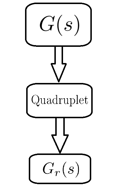
Throughout this paper, a consistent pattern has emerged in all the discussed data-driven algorithms: each algorithm constructs a Loewner quadruplet (in the frequency domain) or an impulse data quadruplet (in the time domain) and then reduces the respective data quadruplet, as illustrated in Figure 1.

Refer to caption — Figure 1: Working Principle

It is now evident that all interpolatory low-rank BT algorithms, including Krylov-subspace-based low-rank BT, low-rank ADI-based BT, and QuadBT, construct the ROM by reducing the corresponding data quadruplets rather than directly reducing the original system. In intrusive settings, these quadruplets are not explicitly constructed, as the low-rank factor $\hat{Z}_{p}$ is derived from the matrices $(E,A,B)$ separately, and the low-rank factor $\hat{Z}_{q}$ is obtained from the matrices $(E,A,C)$ separately. In other words, the input and output dynamics are approximated independently. However, in non-intrusive settings, the true implicit nature of interpolatory low-rank BT algorithms becomes apparent, revealing that they construct the ROM by reducing the data quadruplets rather than directly reducing the original system.

Before proceeding further, let us make an assumption that $mn_{p}=pn_{q}$ , ensuring that the Loewner quadruplets are interpolants of $G(s)$ . This assumption will greatly simplify our discussion, as it allows us to use the terms Loewner quadruplet and interpolant of $G(s)$ interchangeably. Consequently, we can analyze the Loewner quadruplet using standard interpolation theory.

The following observations can be made regarding interpolatory low-rank BT methods:

1.

Similar to numerical integration, interpolatory low-rank BT does not reduce $G(s)$ directly. Instead, an interpolant of $G(s)$ is first implicitly constructed (or explicitly constructed in non-intrusive data-driven settings). This interpolant is not particularly compact, as it is constructed to interpolate $G(s)$ at several interpolation points to capture the majority of the original system’s dynamics. Subsequently, this interpolant acts as a surrogate for $G(s)$ . The ROMs produced by these low-rank BT algorithms are approximations of the interpolants of $G(s)$ , rather than $G(s)$ itself. In this sense, low-rank BT could be termed “numerical BT” if we wish to adopt terminology analogous to numerical integration.
2.

Since a balanced realization is a specific type of state-space representation of $G(s)$ , constructing such a realization without access to any state-space representation of $G(s)$ appears inherently unnatural. QuadBT and the data-driven BT algorithms proposed in this paper essentially first construct a state-space realization of the interpolant of $G(s)$ and then reduce these interpolants rather than the original system. These algorithms are non-intrusive but they perform intrusive MOR on the interpolant of $G(s)$ , for which a state-space realization can be conveniently obtained non-intrusively within the Loewner framework. Their non-intrusive nature does not stem from the fact that Hankel singular values are transfer function parameters and independent of a specific state-space realization, as argued in [11]. Instead, the balanced square-root algorithm remains intrinsically intrusive. Even in QuadBT, it operates on the intrusive state-space realization of the interpolant of $G(s)$ , which interpolates $G(s)$ at the quadrature nodes. In conclusion, BT of $G(s)$ is still only achievable intrusively. What can be performed non-intrusively is the interpolation within the Loewner framework.
3.

In [11], it was argued that rational interpolation does not play a role in QuadBT. However, it is now evident that rational interpolation plays a key role in QuadBT, as it supplies QuadBT with a state-space realization. This realization is then further reduced using the square root algorithm.
4.

Since the ROMs produced by interpolatory low-rank BT are approximations of the interpolants of $G(s)$ , it is unreasonable to expect that reducing the order of the interpolant will result in a final ROM that is more accurate than the interpolant itself. Therefore, the accuracy of the approximation in low-rank BT is directly tied to the quality of the interpolant of $G(s)$ . To ensure that low-rank BT generates ROMs nearly equivalent to those produced by standard BT, the interpolation quality must be exceptional, which heavily relies on the selection of interpolation points. Given that IRKA is regarded as one of the most effective interpolation algorithms, its ROMs should be considered strong candidates for performing low-rank BT. This is supported by [21], where IRKA is used to generate effective shifts for the ADI method.
5.

There is some interest within the MOR community to produce BT models through interpolation; see [40, 41]. These efforts are primarily focused on constructing exact BT models using interpolation techniques. However, it is important to recognize that, in an approximate sense, low-rank BT algorithms are already producing BT models via interpolation. When we acknowledge the success of ADI-based or Krylov-subspace-based algorithms in extending the applicability of BT to large-scale systems by reducing computational costs, we are indirectly affirming that interpolation at a small number of points may not surpass BT in accuracy. However, if interpolation is performed more liberally, it can achieve sufficient accuracy to compete with BT. Interpolation at a large number of points, while powerful, introduces its own complexities, which will be discussed shortly. Nevertheless, the accuracy and effectiveness of interpolation as a tool in MOR must be acknowledged.
6.

The data-driven IRKA algorithms presented in this paper leverage the same principles as low-rank BT. They compute an interpolant of $G(s)$ by interpolating at several points to capture the majority of the dynamics of $G(s)$ . This interpolant then serves as a surrogate for $G(s)$ , allowing the algorithms to sample the interpolant as IRKA updates the interpolation points, rather than directly sampling $G(s)$ . This approach enables the data-driven IRKA algorithms to bypass the need for new experiments to obtain additional samples of $G(s)$ .

Having established that all interpolatory low-rank BT algorithms essentially reduce their respective data quadruplets, one might consider directly applying standard MOR algorithms like BT and IRKA to these quadruplets to obtain a compact ROM. However, these quadruplets are often not as well-behaved as desired. In many cases, when constructing an interpolant in the Loewner framework with a large number of interpolation points, the resulting interpolant is an unstable system with several poles in the right-half plane [7, 22]. As a result, standard MOR algorithms that require a stable original model cannot be directly applied to reduce the size of these quadruplets. Additionally, the Loewner matrix $W^{T}EV$ tends to become singular as the number of interpolation points increases [7, 22], rendering MOR algorithms that assume the non-singularity of the $E$ -matrix unsuitable for directly reducing the order of Loewner interpolants. QuadBT and the algorithms proposed in this paper can be viewed as “compression” algorithms, designed to extract a compact ROM from these quadruplets. Moreover, these algorithms can also be seen as “distillation” algorithms, as they can extract ROMs with various properties from the same “raw” quadruplet by processing it differently. They effectively distill a compact, useful, and well-behaved ROM from the raw data quadruplets, which cannot be directly handled by standard MOR algorithms that assume the original model is well-behaved (like stable and minimal). This opens an interesting avenue for future research: developing similar compression strategies in intrusive settings to handle original systems that are similarly ill-behaved, much like these data quadruplets.

10 Numerical Examples

In this section, the performance of the proposed algorithms is compared with their intrusive counterparts, i.e., BT and IRKA. The first example comprises numerical results related to continuous time algorithms while the second example comprises numerical results related to discrete-time algorithms.

10.1 Experimental Setup

For quadrature-based algorithms, QuadBT [11] is first used to generate ROMs. Subsequently, the proposed quadrature-based IRKA algorithms compress and distill the same quadruplet produced by QuadBT to extract $\mathcal{H}_{2}$ -optimal ROMs. The mirror images of the poles of the ROM obtained from frequency-domain QuadBT are used as sampling points for the quadruplets distilled by DD-ADI-BT and PORK-IRKA. Similarly, the reciprocals of the poles of the ROM from frequency-domain QuadBT serve as sampling points for the quadruplets distilled by DD-PORK-DTBT and PORK-DTIRKA. Both BT and IRKA algorithms compress and distill the same raw quadruplet to extract their respective ROMs. All IRKA-based algorithms are initialized arbitrarily, and they converge within 20 iterations for all experiments conducted in this section. The results presented here are generated using MATLAB R2021b on a laptop running Windows 11 as the operating system, equipped with a 2GHz Intel i7 processor and 16GB of RAM.

10.2 Example 1: Continuous Time

In this example, we use the $120^{th}$ -order CD player model, which has two inputs and two outputs, from the benchmark collection of [42], to compare the performance of the proposed algorithms with intrusive BT, IRKA, and QuadBT. First, using the exponential trapezoidal rule (the numerical quadrature method preferred in [11] for achieving high accuracy), $50$ nodes and weights are generated within the frequency range of $10^{-2}$ to $10^{2}$ rad/sec for frequency-domain QuadBT. The same nodes are used to approximate both the controllability and observability Gramians. Transfer function samples at these nodes are generated using the state-space realization of the CD player model provided in [42]. For time-limited QuadBT, $100$ nodes and weights are generated within the time interval of $0$ to $40$ seconds using the Gauss-Legendre quadrature rule. Impulse response samples are generated using the state-space realization of the CD player model available in [42]. Using this data, the respective quadruplets are constructed and used to execute QuadBT. Subsequently, $22$ ADI shifts are generated as described in subsection 10.1. Transfer function samples are then generated, and the associated quadruplet is constructed.

The largest $20$ Hankel singular values approximated by QuadBT and DD-ADI-BT are shown in Figure 2.

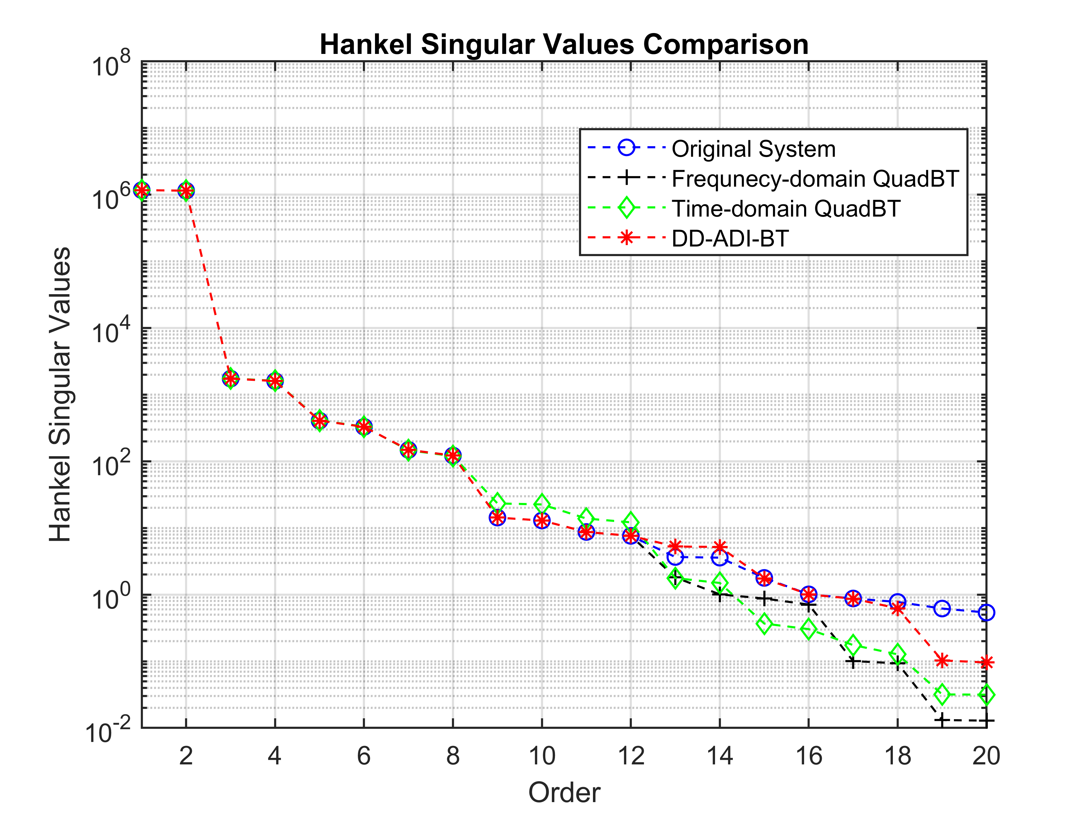
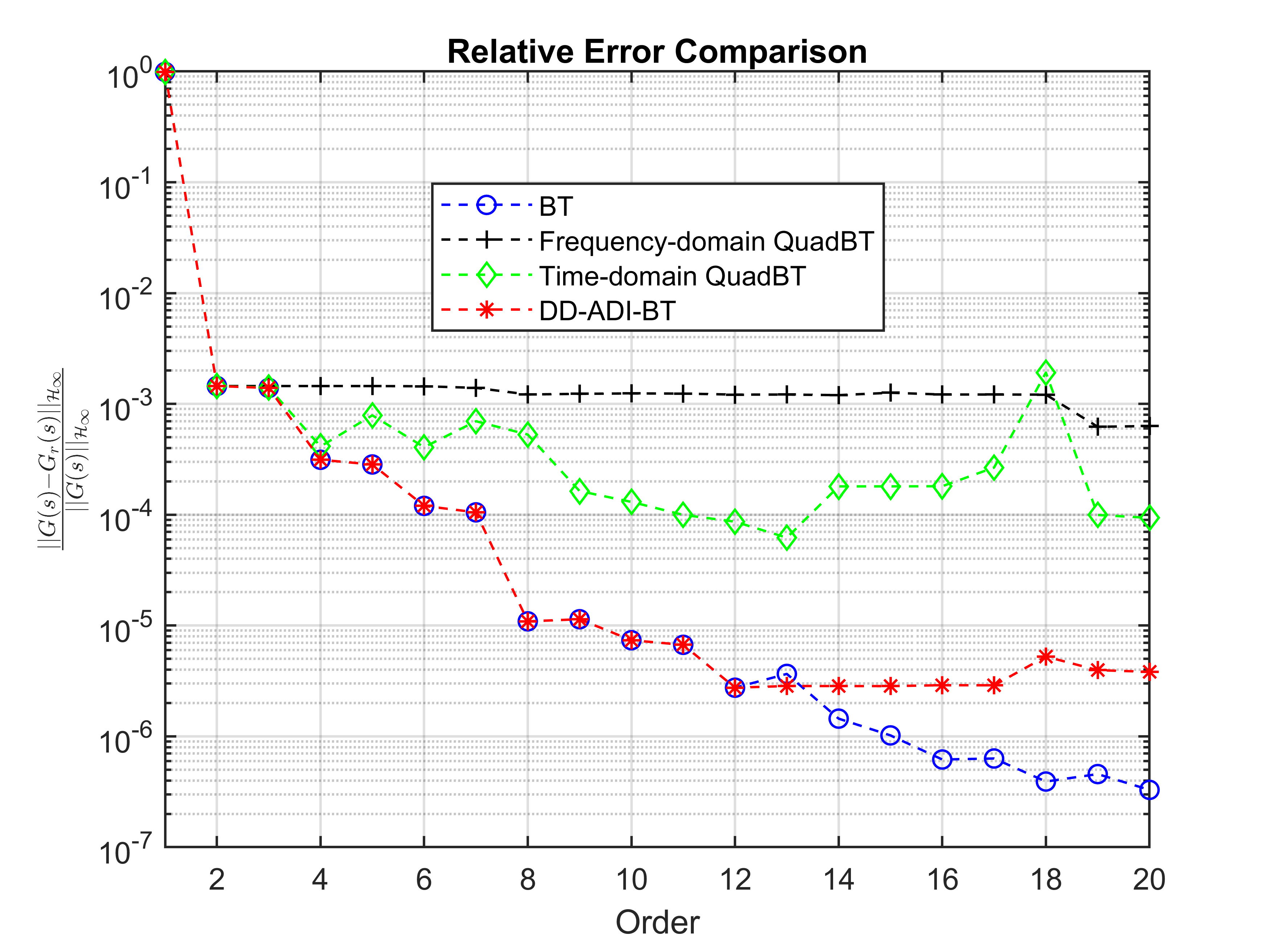
It can be seen that DD-ADI-BT closely approximates the majority of the Hankel singular values while using fewer than half the number of transfer function samples. This result is expected, as ADI-based BT is known to provide accurate approximations even with a limited number of shifts. The $\mathcal{H}_{\infty}$ norm of the relative error $\frac{||G(s)-G_{r}(s)||_{\mathcal{H}_{\infty}}}{||G(s)||_{\mathcal{H}_{\infty}}}$ for ROMs of orders $1-20$ is displayed in Figure 3. It can be observed that DD-ADI-BT performs comparably to intrusive BT in terms of accuracy and outperforms QuadBT in this example.

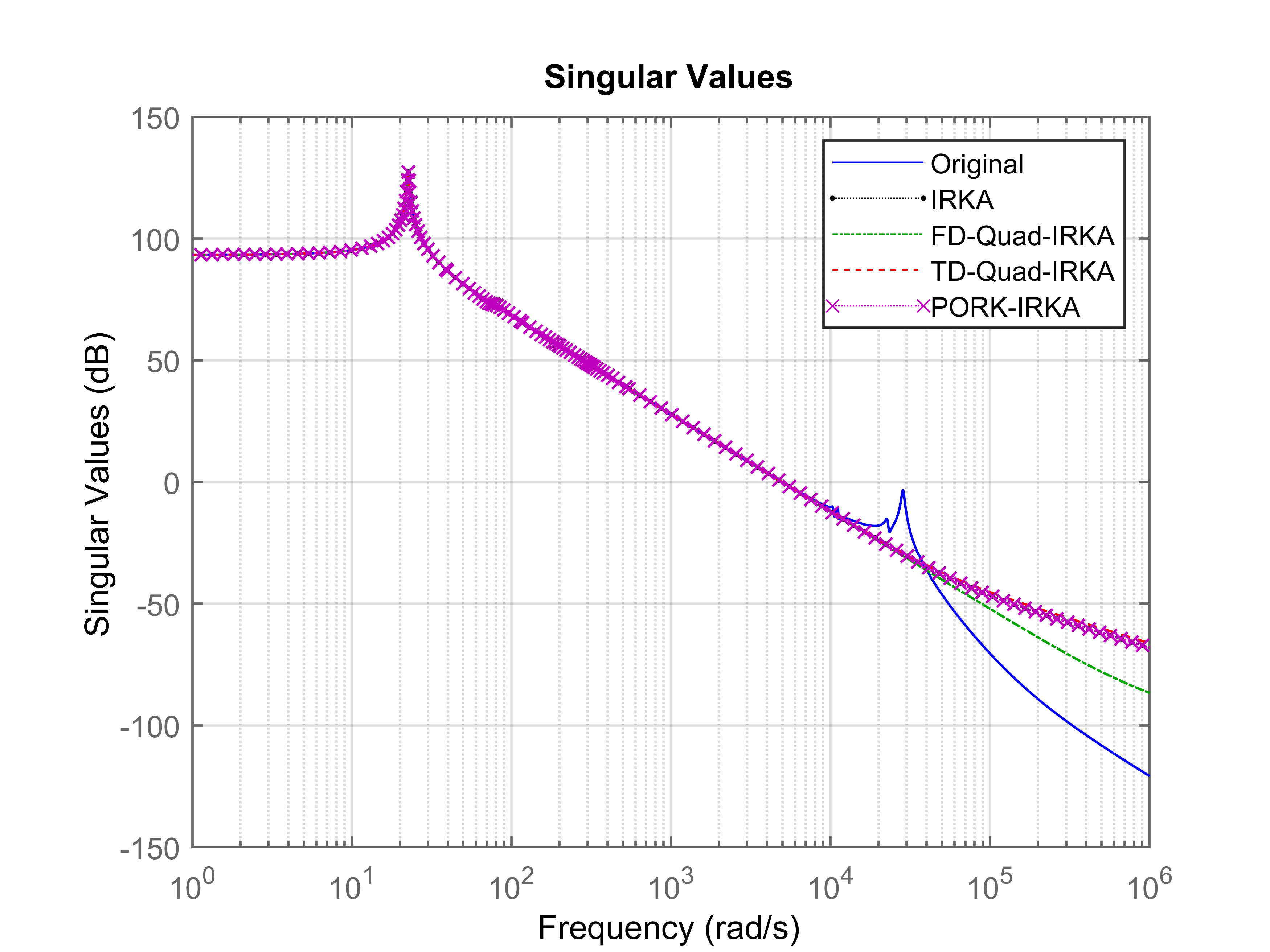
Using the same respective quadruplets, FD-Quad-IRKA, TD-Quad-IRKA, and PORK-IRKA are used to extract an $8^{th}$ -order ROM. The weights in FD-Quad-IRKA and TD-Quad-IRKA are computed using trapezoidal rule for the same nodes used by QuadBT. Figure 4 displays the singular values of $G(s)$ (for input 1 and output 1) and the ROMs $G_{r}(s)$ generated by IRKA, FD-Quad-IRKA, TD-Quad-IRKA, and PORK-IRKA. It is evident that the proposed algorithms achieve accuracy comparable to that of IRKA. For economy of space, only the frequency response of the $1^{st}$ input-output channel is plotted.

10.3 Example 2: Discrete Time

For this example, we use the model considered in [11], which is a $40^{th}$ -order low-pass Butterworth filter with a cutoff frequency of $0.6$ rad/sec. First, using the Gauss-Legendre quadrature rule, $100$ nodes and weights are generated within the frequency range of $-\pi$ to $\pi$ rad/sec for frequency-domain QuadBT. These nodes are used to approximate both the controllability and observability Gramians. Transfer function samples at these nodes are generated using the state-space realization of the Butterworth filter model, created using MATLAB’s ‘butter’ command. For time-limited QuadBT, $100$ impulse response samples are generated. Using this data, the respective quadruplets are constructed and used to implement QuadBT. Subsequently, $20$ PORK shifts are generated as described in subsection 10.1. Transfer function samples are then generated, and the associated quadruplet is constructed.

The largest $20$ Hankel singular values approximated by QuadBT and DD-PORK-DTBT are shown in Figure 5.

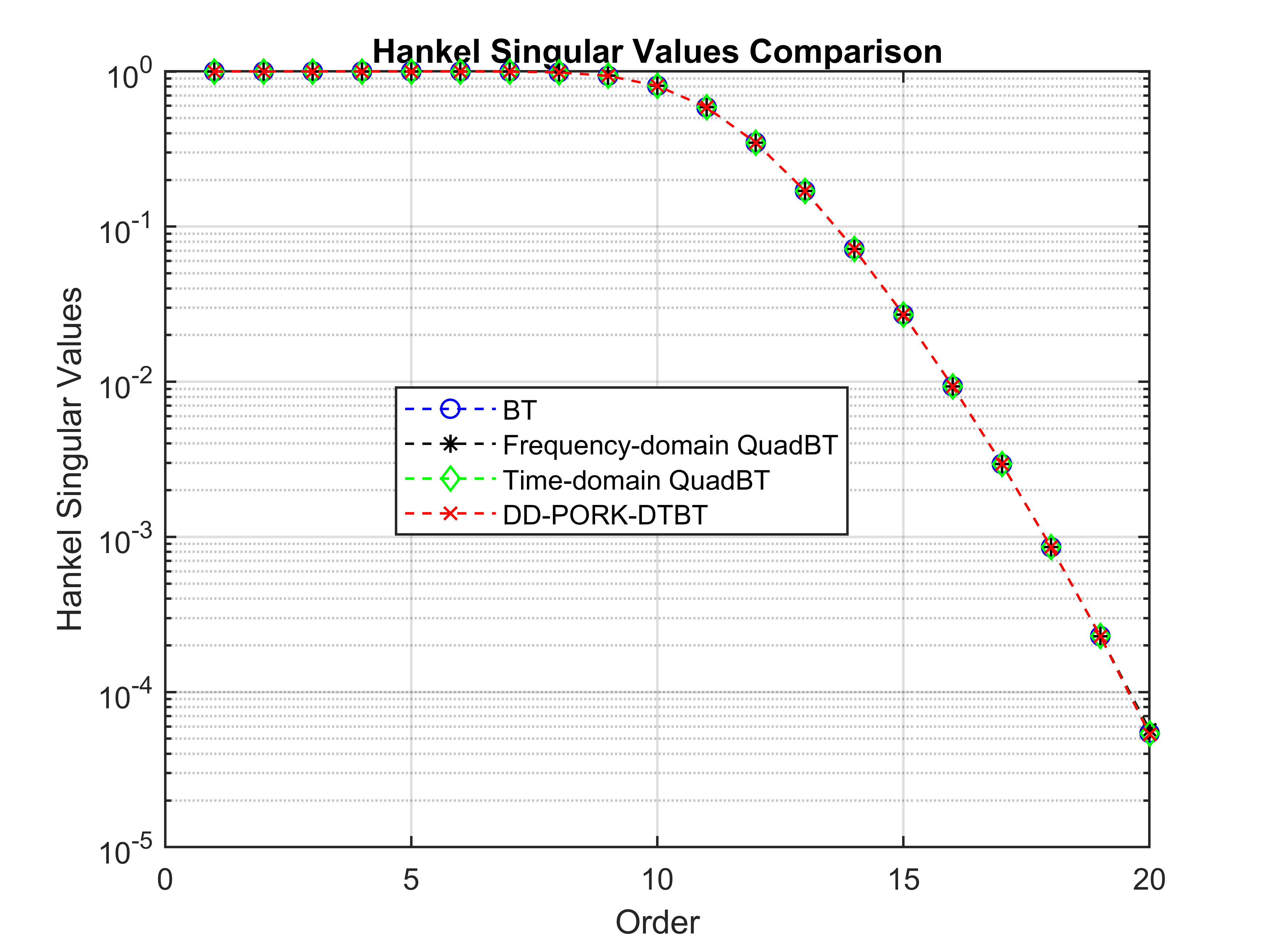
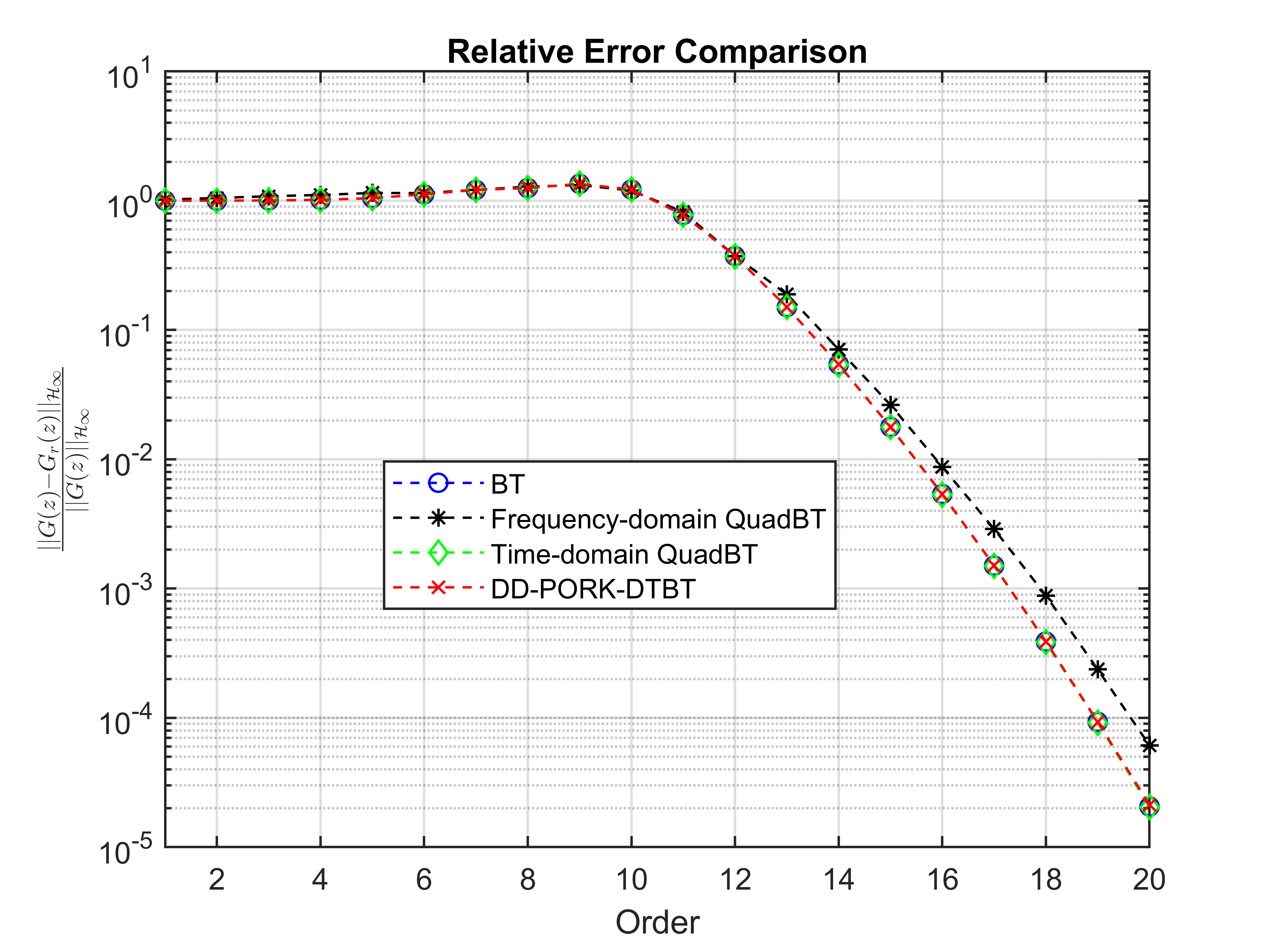
It can be seen that DD-PORK-DTBT closely approximates all the $20$ Hankel singular values while using fewer transfer function samples. The $\mathcal{H}_{\infty}$ norm of the relative error $\frac{||G(z)-G_{r}(z)||_{\mathcal{H}_{\infty}}}{||G(z)||_{\mathcal{H}_{\infty}}}$ for ROMs of orders $1-20$ is displayed in Figure 6. It can be observed that DD-PORK-DTBT performs comparably to intrusive BT in terms of accuracy.

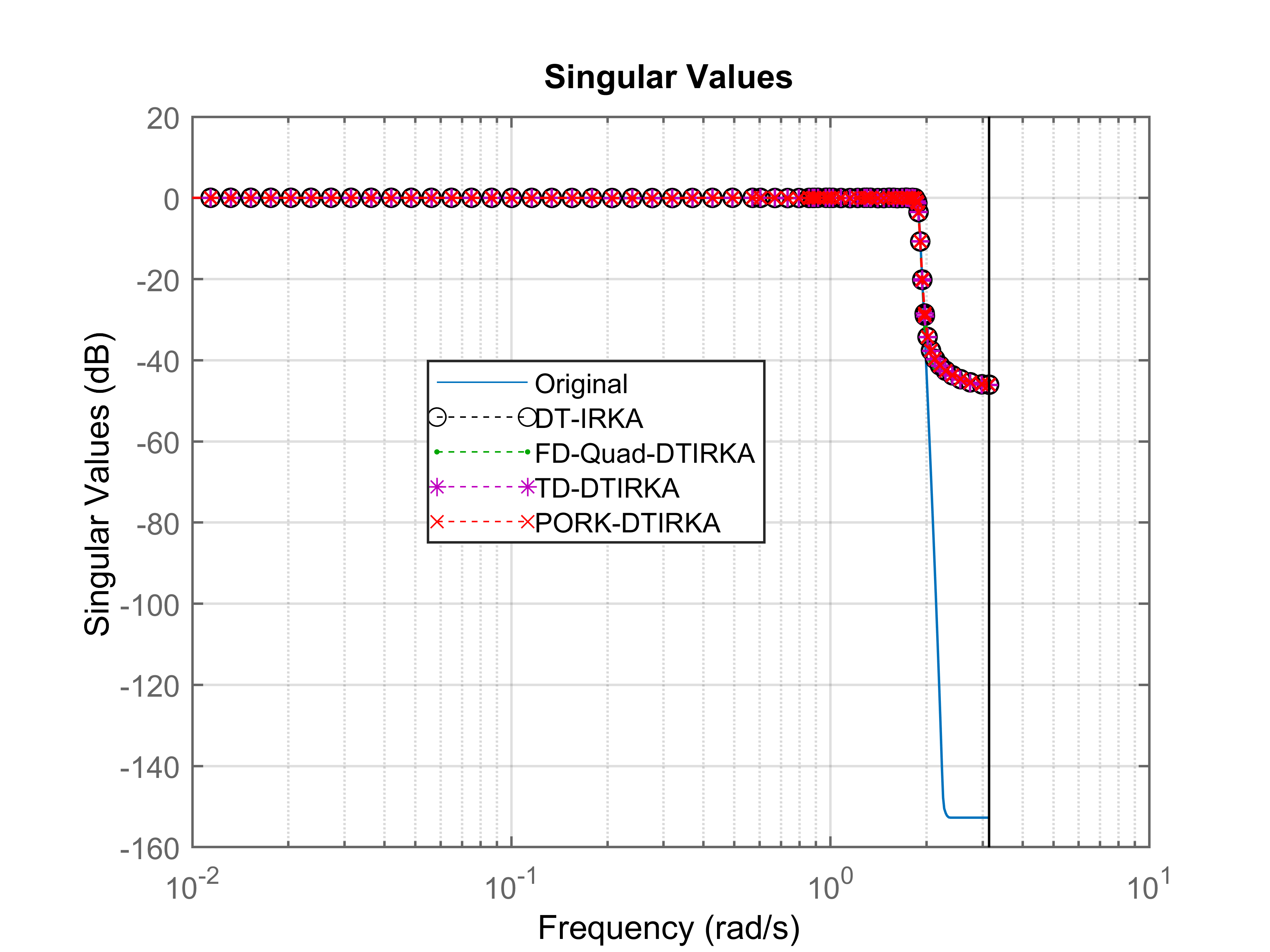
Using the same respective quadruplets, FD-Quad-DTIRKA, TD-DTIRKA, and PORK-DTIRKA are used to extract an $15^{th}$ -order ROM. The weights in FD-Quad-DTIRKA are computed using trapezoidal rule for the same nodes used by QuadBT. Figure 7 displays the singular values of $G(s)$ and the ROMs $G_{r}(s)$ generated by DT-IRKA, FD-Quad-DTIRKA, TD-DTIRKA, and PORK-DTIRKA. It is evident that the proposed algorithms achieve accuracy comparable to that of DT-IRKA.

11 Conclusion

This paper presents data-driven, non-intrusive implementations of BT and IRKA for both continuous-time and discrete-time systems. The proposed methods utilize available frequency or time-domain data to compute ROMs. It has been observed that both QuadBT and the algorithms introduced in this paper effectively compress and distill their respective raw quadruplets, resulting in compact and practical ROMs. Numerical experiments demonstrate that the proposed algorithms perform comparably to their intrusive counterparts.

References

[1] A. C. Antoulas, S. Lefteriu, A. C. Ionita, P. Benner, A. Cohen, A tutorial introduction to the Loewner framework for model reduction, Model Reduction and Approximation: Theory and Algorithms 15 (2017) 335.
[2] G. Obinata, B. D. Anderson, Model reduction for control system design, Springer Science & Business Media, 2012.
[3] A. C. Antoulas, Approximation of large-scale dynamical systems, SIAM, 2005.
[4] B. Moore, Principal component analysis in linear systems: Controllability, observability, and model reduction, IEEE Transactions on Automatic Control 26 (1) (1981) 17–32.
[5] P. Benner, J. Saak, Numerical solution of large and sparse continuous time algebraic matrix Riccati and Lyapunov equations: A state of the art survey, GAMM-Mitteilungen 36 (1) (2013) 32–52.
[6] V. Simoncini, Computational methods for linear matrix equations, SIAM Review 58 (3) (2016) 377–441.
[7] A. Mayo, A. C. Antoulas, A framework for the solution of the generalized realization problem, Linear Algebra and Its Applications 425 (2-3) (2007) 634–662.
[8] Y. Nakatsukasa, O. Sète, L. N. Trefethen, The AAA algorithm for rational approximation, SIAM Journal on Scientific Computing 40 (3) (2018) A1494–A1522.
[9] I. V. Gosea, C. Poussot-Vassal, A. C. Antoulas, Data-driven modeling and control of large-scale dynamical systems in the Loewner framework: Methodology and applications, in: Handbook of Numerical Analysis, Vol. 23, Elsevier, 2022, pp. 499–530.
[10] G. Scarciotti, A. Astolfi, Interconnection-based model order reduction-A survey, European Journal of Control 75 (2024) 100929.
[11] I. V. Gosea, S. Gugercin, C. Beattie, Data-driven balancing of linear dynamical systems, SIAM Journal on Scientific Computing 44 (1) (2022) A554–A582.
[12] S. Gugercin, A. C. Antoulas, C. Beattie, $\mathcal{H}_{2}$ model reduction for large-scale linear dynamical systems, SIAM Journal on Matrix Analysis and Applications 30 (2) (2008) 609–638.
[13] C. Beattie, S. Gugercin, Realization-independent $\mathcal{H}_{2}$ -approximation, in: 2012 IEEE 51st IEEE Conference on Decision and Control (CDC), IEEE, 2012, pp. 4953–4958.
[14] T. Wolf, H. K. Panzer, B. Lohmann, $\mathcal{H}_{2}$ pseudo-optimality in model order reduction by Krylov subspace methods, in: 2013 European Control Conference (ECC), IEEE, 2013, pp. 3427–3432.
[15] T. Wolf, $\mathcal{H}_{2}$ pseudo-optimal model order reduction, Ph.D. thesis, Technische Universität München (2014).
[16] P. Benner, P. Kürschner, J. Saak, Efficient handling of complex shift parameters in the low-rank Cholesky factor ADI method, Numerical Algorithms 62 (2013) 225–251.
[17] J. Saak, P. Benner, P. Kürschner, A goal-oriented dual LRCF-ADI for balanced truncation, IFAC Proceedings Volumes 45 (2) (2012) 752–757.
[18] C. A. Beattie, S. Gugercin, et al., Model reduction by rational interpolation, Model Reduction and Approximation 15 (2017) 297–334.
[19] M. S. Tombs, I. Postlethwaite, Truncated balanced realization of a stable non-minimal state-space system, International Journal of Control 46 (4) (1987) 1319–1330.
[20] T. Wolf, H. K. Panzer, The ADI iteration for Lyapunov equations implicitly performs $\mathcal{H}_{2}$ pseudo-optimal model order reduction, International Journal of Control 89 (3) (2016) 481–493.
[21] P. Benner, P. Kürschner, J. Saak, Self-generating and efficient shift parameters in ADI methods for large lyapunov and sylvester equations, Electronic Transactions on Numerical Analysis 43 (2014) 142–162.
[22] J. Mao, G. Scarciotti, Data-driven model reduction by two-sided moment matching, Automatica 166 (2024) 111702.
[23] L. Lennart, System identification: Theory for the user, Vol. 28, 1999.
[24] H. Özbay, S. Gümüşsoy, K. Kashima, Y. Yamamoto, Frequency Domain Techniques for $\mathcal{H}_{\infty}$ Control of Distributed Parameter Systems, SIAM, 2018.
[25] R. Pintelon, J. Schoukens, Y. Rolain, Frequency-domain approach to continuous-time system identification: Some practical aspects, Identification of Continuous-time models from Sampled Data (2008) 215–248.
[26] J. Gillberg, Frequency domain identification of continuous-time systems: Reconstruction and robustness, Ph.D. thesis, Institutionen för systemteknik (2006).
[27] E. A. Morelli, J. A. Grauer, Practical aspects of frequency-domain approaches for aircraft system identification, Journal of Aircraft 57 (2) (2020) 268–291.
[28] D. C. Sorensen, A. Antoulas, The Sylvester equation and approximate balanced reduction, Linear Algebra and Its Applications 351 (2002) 671–700.
[29] U. Zulfiqar, V. Sreeram, X. Du, Frequency-limited pseudo-optimal rational Krylov algorithm for power system reduction, International Journal of Electrical Power & Energy Systems 118 (2020) 105798.
[30] G.-B. Stan, J.-J. Embrechts, D. Archambeau, Comparison of different impulse response measurement techniques, Journal of the Audio Engineering Society 50 (4) (2002) 249–262.
[31] R. J. Finno, S. L. Gassman, Impulse response evaluation of drilled shafts, Journal of Geotechnical and Geoenvironmental Engineering 124 (10) (1998) 965–975.
[32] M. Holters, T. Corbach, U. Zölzer, Impulse response measurement techniques and their applicability in the real world, In: Proceedings of the 12th International Conference on Digital Audio Effects (DAFx-09), 2009, pp. 108–112.
[33] S. Foster, Impulse response measurement using golay codes, In: ICASSP’86. IEEE International Conference on Acoustics, Speech, and Signal Processing, Vol. 11, IEEE, 1986, pp. 929–932.
[34] J. Borish, J. B. Angell, An efficient algorithm for measuring the impulse response using pseudorandom noise, Journal of the Audio Engineering Society 31 (7/8) (1983) 478–488.
[35] U. Zulfiqar, V. Sreeram, X. Du, Time-limited pseudo-optimal-model order reduction, IET Control Theory & Applications 14 (14) (2020) 1995–2007.
[36] P. Benner, M. Köhler, J. Saak, Sparse-dense Sylvester equations in $\mathcal{H}_{2}$ -model order reduction, Preprint MPIMD/11-11, Max Planck Institute Magdeburg, available from http://www.mpi-magdeburg.mpg.de/preprints/ (Dec. 2011).
[37] A. Bunse-Gerstner, D. Kubalińska, G. Vossen, D. Wilczek, $\mathcal{H}_{2}$ -norm optimal model reduction for large scale discrete dynamical MIMO systems, Journal of Computational and Applied Mathematics 233 (5) (2010) 1202–1216.
[38] M. S. Ackermann, S. Gugercin, Time-domain iterative rational Krylov method, arXiv preprint arXiv:2407.12670 (2024).
[39] G.-R. Duan, Generalized Sylvester equations/g, R. Duan. Unified Parametric Solutions: CRC Press, Boca Raton, FL (2015).
[40] T. C. Ionescu, J. M. Scherpen, O. V. Iftime, A. Astolfi, Balancing as a moment matching problem, in: Proc. 20th int. symp. On Mathematical Theory of Networks and Sys, 2012.
[41] Y. Kawano, T. C. Ionescu, O. V. Iftime, Gramian preserving moment matching for linear systems, In: 2023 European Control Conference (ECC), IEEE, 2023, pp. 1–6.
[42] Y. Chahlaoui, P. V. Dooren, Benchmark examples for model reduction of linear time-invariant dynamical systems, in: Dimension reduction of large-scale systems, Springer, 2005, pp. 379–392.

	$\displaystyle\|\|G(s)$	$\displaystyle-G_{r}(s)^{(i-1)}\|\|_{\mathcal{H}_{2}}^{2}$
	$\displaystyle=$	$\displaystyle\|\|G(s)\|\|_{\mathcal{H}_{2}}^{2}+\|\|G_{r}(s)^{(i-1)}\|\|_{\mathcal{H}_{2}}^{2}-2\text{trace}\Big{(}C_{r}^{(i)}\big{(}C_{r}^{(i-1)}T_{r}^{(i-1)}\big{)}^{*}\Big{)}.$

Compression and Distillation of Data Quadruplets in Non-intrusive Reduced-order Modeling

Abstract

keywords:

1 Introduction

2 Preliminaries

2.1 Review of Interpolation Theory [18]

2.2 Iterative Rational Krylov Algorithm (IRKA) [12]

2.3 Pseudo-optimal Rational Krylov (PORK) Algorithm [15]

2.4 Interpolatory Loewner framework [7]

2.5 Balanced Truncation (BT) [4]

2.6 Data-driven Quadrature-based Balanced Truncation (QuadBT)[11]

3 Low-rank ADI-based Non-intrusive Balanced Truncation for Continuous-time Systems

4 Data-driven Implementations of IRKA for Continuous-time Systems

4.1 Using Available Frequency Response Data

4.2 Using Available Impulse Response Data

4.3 Using Available Transfer Function Samples

4.4 Tracking the Error ‖G​(s)−Gr​(s)‖ℋ2||G(s)-G_{r}(s)||_{\mathcal{H}_{2}}

5 Data-driven Implementations of IRKA for Discrete-time Systems

5.1 Using Available Frequency Response Data

5.2 Using Available Impulse Response Data

6 Pseudo-optimal Rational Krylov (PORK) Algorithm for Discrete-time Systems

6.1 Input PORK (I-PORK)

Theorem 6.1.

Proof.

6.2 Output PORK (O-PORK)

Theorem 6.2.

Proof.

6.3 Approximation of Gramians

7 Non-intrusive PORK-based Low-rank Balanced Truncation for Discrete Time Systems

8 Non-intrusive PORK-based DT-IRKA for Discrete Time Systems

8.1 Tracking the Error ‖G​(z)−Gr​(z)‖ℋ22||G(z)-G_{r}(z)||_{\mathcal{H}_{2}}^{2}

9 Compression and Distillation of Data Quadruplets

10 Numerical Examples

10.1 Experimental Setup

10.2 Example 1: Continuous Time

10.3 Example 2: Discrete Time

11 Conclusion

References

4.4 Tracking the Error $||G(s)-G_{r}(s)||_{\mathcal{H}_{2}}$

8.1 Tracking the Error $||G(z)-G_{r}(z)||_{\mathcal{H}_{2}}^{2}$