Compressing Recurrent Neural Networks Using Hierarchical Tucker Tensor Decomposition

Tensor Contraction. An HT-decomposed tensor is essentially the consecutive product of multiple tensor contraction results, where tensor contraction is executed between two tensors with at least one matched dimension. For instance, given two tensors $\bm{\mathcal{A}}\in\mathbb{R}^{n_{1}\times n_{2}\times l}$ and $\bm{\mathcal{B}}\in\mathbb{R}^{l\times m_{1}\times m_{2}}$, where the 3rd dimension of $\bm{\mathcal{A}}$ matches the 1st dimension of $\bm{\mathcal{B}}$ with length $l$, the tensor contraction result is a size- $n_{1}\times n_{2}\times m_{1}\times m_{2}$ tensor as

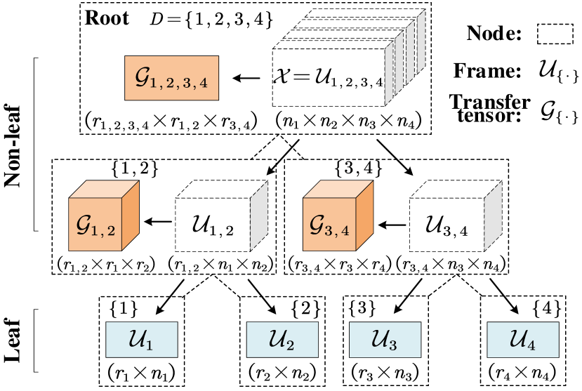
Hierarchical Tucker Decomposition. The Hierarchical Tucker decomposition is a special type of tensor decomposition approach with hierarchical levels with respect to the order of the tensor. As illustrated in Figure 1, an HT-decomposed tensor can be recursively decomposed into intermediate components, referred as frames, from top to bottom in a binary tree, where each frame corresponds to a unique node, and each node is associated with a dimension set. In general, for a HT-decomposed tensor $\bm{\mathcal{X}}\in\mathbb{R}^{n_{1}\times\cdots\times n_{d}}$, we can build a binary tree with a root node associated with $D=\{1,2,\cdots,d\}$ and $\bm{\mathcal{X}}=\bm{\mathcal{U}}_{D}$ as the root frame. For each non-leaf frame $\bm{\mathcal{U}}_{s}\in\mathbb{R}^{r_{s}\times n_{\mu_{s}}\times\cdots\times n_{\nu_{s}}}$, where $s\subsetneq D$ is associated with the node corresponding to $\bm{\mathcal{U}}_{s}$ , $s_{1},s_{2}\subsetneq s$ are associated with the left and right child nodes of the $s$-associated node, and $\mu_{s}=\min(s),\nu_{s}=\max(s)$, $\bm{\mathcal{U}}_{s}$ can be recursively decomposed to its left and right child frames ($\bm{\mathcal{U}}_{s_{1}}$ and $\bm{\mathcal{U}}_{s_{2}}$) and transfer tensor $\bm{\mathcal{G}}_{s}\in\mathbb{R}^{r_{s}\times r_{s_{1}}\times r_{s_{2}}}$ as

Consequently, by performing this recursive decomposition till the bottom of the binary tree, we can decompose the original ${n_{1}\times\cdots\times n_{d}}$-order tensor $\bm{\mathcal{X}}=\bm{\mathcal{U}}_{D}$ into the combination of the 2-order leaf frames and 3-order transfer tensors. Notice that here $r_{s}$, as hierarchical rank, is an important parameter that determines the decomposition effect.

This subsection describes the details of compressing the large-size RNN models to the compact ones using HT decomposition, including the key steps as well as the important HT-based forward and backward propagation schemes.

Tensorization. In general, the key idea of building HT-RNN is to transform the weight matrix $\bm{W}\in\mathbb{R}^{M\times N}$ to the HT-based format. Considering $\bm{W}$ is a 2-D matrix, while HT decomposition is mainly performed on high-order tensor, we first need to reshape $\bm{W}$ as well as its affiliated input vector $\bm{x}\in\mathbb{R}^{N}$ and output vector $\bm{y}\in\mathbb{R}^{M}$ to tensor format as $\bm{\mathcal{W}}\in\mathbb{R}^{m_{1}\times\cdots\times m_{d}\times n_{1}\times\cdots\times n_{d}}$, $\bm{\mathcal{X}}\in\mathbb{R}^{n_{1}\times\cdots\times n_{d}}$ and $\bm{\mathcal{Y}}\in\mathbb{R}^{m_{1}\times\cdots\times m_{d}}$, respectively, where $M=\prod_{i=1}^{d}m_{i}$ and $N=\prod_{j=1}^{d}n_{j}$.

Decomposing $\bm{W}$. Given a tensorized $\bm{W}$ as $\bm{\mathcal{W}}\in\mathbb{R}^{m_{1}\times\cdots\times m_{d}\times n_{1}\times\cdots\times n_{d}}$, we can now leverage HT decomposition to represent the large-size $\bm{W}$ using a set of small-size matrices and tensors. In general, following Equation (1), $\bm{\mathcal{W}}$ can be decomposed as

where $\varphi_{s}(\bm{i},\bm{j})$ is a mapping function that produces the correct indices $\bm{i}=(i_{1},\cdots,i_{d})$ and $\bm{j}=(j_{1},\cdots,j_{d})$ for a specified frame $\bm{\mathcal{U}}_{s}$ with the given $s$ and $d$. For instance, with $d=6$ and $s=\{3,4\}$, the output of $\varphi_{s}(\bm{i},\bm{j})$ is $(i_{3},i_{4},j_{3},j_{4})$. In addition, $\bm{\mathcal{U}}_{D_{1}}$ and $\bm{\mathcal{U}}_{D_{2}}$ can be recursively computed as

where $D=\{1,2,\cdots,d\}$, $D_{1}=\{1,\cdots,\lfloor d/2\rfloor\}$ and $D_{2}=\{\lceil d/2\rceil,\cdots,d\}$ are associated with left and right child nodes of the root node.

HT Layer. With the HT-decomposed weight matrix, the component HT layer of HT-based RNN models can now be developed. Specifically, the HT-format matrix-vector multiplication, as the kernel computation in the forward propagation procedure, is performed as follows:

Considering the desired output $\bm{y}$ of HT-layer is a vector, the calculated $\bm{\mathcal{Y}}$ needs to be re-shaped again to the 1-D format. Consequently, we denote the entire forward computing procedure from input $\bm{x}$ to output $\bm{y}$ as

Remark-1: Hierarchical Structure in HT-layer. In tensor theory both the tensors and their computations can be graphically represented using tensor diagram (see Figure 2(a)). For HT decomposition, its inherent hierarchical characteristics make the corresponding HT-layer exhibit strong multi-level hierarchical structure, which is visualized in the specific tensor diagram of HT-layer (see Figure 2(b)). Considering that a well-known feature and advantage of deep neural network is its strong ability of capturing hierarchical pattern and representation via its multi-layer structure, the existence of such hierarchical structure in HT-layer can effectively improve the representation capability of the overall neural network models. In Section 3, empirical experiments on different datasets demonstrate that HT-based RNN models indeed outperform many other types of RNN models in terms of accuracy. Besides, it is worth noting that some recent advances in learning theory Nadav et al. (2018) also indicates the strong connection and correlation between HT modeling and expressive power of deep neural networks.

HT-LSTM. With the HT-based component layers, a HT-based RNN model can be simply constructed by replacing the original uncompressed layer with the HT-layer. Considering LSTM is the most popular and advanced variant of RNNs, we develop the corresponding HT-LSTM model as follows:

where $\sigma$, $\tanh$ and $\odot$ are the sigmoid function, hyperbolic function and element-wise product, respectively.

HT-based Gradient Calculation. To ensure the valid training on HT-RNN, the gradient calculation in the backward propagation should also be accordingly reformulated to HT-based format. In general, considering for HT layer $\bm{\mathcal{W}}=\bm{\mathcal{U}}_{D}$ and $\frac{\partial\bm{\mathcal{Y}}}{\partial\bm{\mathcal{U}}_{D}}=\bm{\mathcal{X}}$, assuming $s$ is associated with a left node, as we denote that $F(s)$ and $B(s)$ are the sets associated with the father and brother nodes of the $s$-associated node in the binary tree, respectively, and define $\mu_{s}=\min(s),\nu_{s}=\max(s)$, the partial derivative of output tensor with respect to frames can be calculated in the following recursive way until $F(s)$ is equal to $D$:

Based on Equation (7), the gradients for leaf frames and transfer tensors can be computed as follows:

To better understand the impact of HT decomposition on RNNs, we analyze the theoretical complexity of HT-RNN, and compare it with the vanilla uncompressed RNN as well as other tensor decomposition-based RNN models. Table 1 summarizes the space complexity and time complexity of different RNN models. It is seen that compared with the other compressed RNN models using tensor decomposition, HT-RNN has the lowest space complexity to store the model parameters. Meanwhile, HT-RNN also enjoys less time complexity than most listed models for both forward and backward propagation. It is worth noting that though TT-RNN has even less time complexity than HT-RNN, it has weaker representation capability, which translates to the lower accuracy, as demonstrated via the experimental results in Section 3.

Remark-2. Besides theoretical complexity analysis, we also verify the low-cost benefits of HT-based compression via empirical experiments. Figure 3(a) shows the number of parameters to store a compressed weight matrix, and Figure 3(b) shows the number of needed operations for multiplication between the compressed weight matrix and vector. Here we adopt the size-$57,600\times 256$ weight matrix used in Yang et al. (2017) Ye et al. (2018) Pan et al. (2019) for evaluation. From Figure 3 it is seen that HT-based approach indeed achieves lower costs, especially on storage requirement, than other tensor decomposition-based methods. Next, the experiments in Section 3 further show the advantages of HT-based RNN on compression ratios over various datasets.

Hyperparameter Setting. We train the models using ADAM optimizer with L2 regularization of coefficient 0.001. Also, dropout rate is set as 0.25 and batch size is 16.

UCF11 Dataset. The UCF11 dataset Liu et al. (2009) consists of 11-class human action (e.g. biking, diving, basketball) videos with totally 1,600 video clips. Each class is assembled by 25 video groups, where each group contains at least 4 action clips. For each clip, the resolution is $320\times 240$.

At data pre-processing stage we choose the same settings used in the related work Ye et al. (2018) Pan et al. (2019) for fair comparison. Specifically, the resolution of video clips is first scaled down to $160\times 120$, and then 6 frames from each clip are randomly sampled to form the sequential input for our HT-LSTM model.

For the baseline vanilla uncompressed LSTM model, it contains 4 input-to-hidden layers, where the size of its input vector is $160\times 120\times 3=57,600$, and the number of hidden states in each layer is 256. For our proposed HT-LSTM, the input vector is reshaped to a tensor of shape $8\times 10\times 10\times 9\times 8$, and the output tensor of the input-to-hidden layer is of shape $4\times 4\times 2\times 4\times 2$. All leaf ranks are set as 4, and all non-leaf ranks are set as 5.

Table 2 summarizes the performance of our HT-LSTM on UCF11 dataset and compare it with the related work. It is seen that compared with vanilla LSTM using 59 million parameters, HT-LSTM only needs 47,375$\times$ fewer parameters with 17.5% accuracy increase. Compared with the recent advances on compressing RNNs using other tensor decomposition methods, including TT-LSTM, BT-LSTM and TR-LSTM, our proposed HT-LSTM requires at least 1.38$\times$ fewer parameters with at least 0.3% increase in accuracy.

Youtube Celebrities Face Dataset. Youtube dataset Kim et al. (2008) contains 1,910 video clips from 47 subjects, where each of it is a celebrated individual such as movie star. Also, the resolutions of the frames vary for different video clips. Being consistent with prior work, for data pre-processing the resolution of the input data to HT-LSTM is re-scaled as $160\times 120$. Also, 6 frames in each video clips are randomly sampled to form the input sequence.

In this experiment we build a HT-LSTM with the similar setting with the one used in UCF11 dataset. To be specific, 4 input-to-hidden layers are equipped, and the shapes of tensorized input and output vectors are $8\times 10\times 10\times 9\times 8$ and $4\times 4\times 2\times 4\times 2$, respectively. A slight difference is in this HT-LSTM all leaf ranks are set as 3, and all non-leaf ranks are set as 4.

Table 3 compares the performance of HT-LSTM with prior work on Youtube Celebrities Face dataset. Considering among the state-of-the-art work, only TT-RNN Yang et al. (2017), including TT-GRU and TT-LSTM, reports both the accuracy and compression ratio on this dataset, the comparison in Table 3 is mainly between HT-LSTM and TT-based solutions. From this table it is seen that HT-LSTM achieves 72,818$\times$ compression ratio over the original uncompressed LSTM with much higher accuracy. Compared with the existing high-compression model TT-GRU, HT-LSTM has 4.1$\times$ fewer parameters but offering 8.1% accuracy increase.

Besides, on the same Youtube dataset we also compare HT-LSTM with several other reported works without using tensor decomposition method. As shown in Table 4, among those works the state-of-the-art model is Ortiz et al. (2013), which has the highest reported accuracy (80.8%). Compared with that model, HT-LSTM achieves 7.3% higher test accuracy.

Another set of our experiments is based on training strategy using pre-trained CNNs. To be specific, the pre-trained CNN first extracts the useful and compact features from the large-size raw input data, and then sends those captured features to RNN, As indicated in Donahue et al. (2015), using the front-end CNN can not only reduce the required input vector size of RNN, but can also significantly improve the overall performance of the entire CNN+RNN model.

Hyperparameter Setting. In this part of experiments dropout rate is set as 0.5. The L2 regularization with coefficient 0.0001 is used, and the entire HT-LSTM model is trained using ADAM optimizer with batch size 16.

UCF11 Dataset. Consistent with Pan et al. (2019), Inception-V3 is selected as the the front-end CNN feature extractor, whose output is a flattened size-2,048 feature vector. For our proposed HT-LSTM, this feature vector, as the input to the model, is reshaped to a tensor of size $8\times 8\times 8\times 4$. Similarly, the output vector is reshaped to a tensor of size $4\times 8\times 8\times 8$. In addition, the ranks for all the nodes are set as 4.

Table 5 summarizes the test accuracy of different models over UCF11 dataset. It is seen that with pre-trained CNN model as front-end feature extractor, HT-LSTM achieves 98.1% accuracy, which is 3.5% higher than the best reported accuracy from the state of the art. Compared with the TR-LSTM using the same front-end CNN, HT-LSTM achieves 4.3% accuracy increase. Meanwhile, being compressed from the same vanilla LSTM, HT-LSTM model brings very high compression ratio as 12,945; while the compression ratio of TR-LSTM is only 25.

HMDB51 Dataset. HMDB51 dataset Kuehne et al. (2011) contains 6,849 video clips that belong to 51 action categories, where each of them consists of more than 101 clips. Again, for the experiment on this dataset we use Inception-V3 as the pre-trained CNN model, whose extracted feature is flattened to a length-2,048 vector. Reshaped from this vector, the input tensor has size of $8\times 8\times 8\times 4$. We also reshape the output vector to a tensor of size $4\times 8\times 8\times 8$. Meanwhile, the ranks of all the nodes are set as 4.

Table 6 summarizes the performance of CNN-aided HT-LSTM and other related work on this dataset. It is seen that HT-LSTM achieves 64.2% accuracy, which obtains 0.4% increase than the recent TR-LSTM. Meanwhile, the compression ratio brought by HT-LSTM is 12,945, which is much higher than the 25$\times$ parameter reduction in TR-LSTM.

It is worth noting that the state-of-the-art work Carreira and Zisserman (2017) achieves a higher accuracy (66.4%) than HT-LSTM. This performance is based on using two streams of input (RGB images and optical flow); while HT-LSTM does not utilize optical flow information of the video. When only RGB information of the video is sent to the models, HT-LSTM can achieve very competitive classification performance as compared to the prior work.

References

- Carreira and Zisserman [2017] Joao Carreira and Andrew Zisserman. Quo vadis, action recognition? a new model and the kinetics dataset. In Proceedings of the IEEE Conference on Computer Vision and Pattern Recognition, pages 6299–6308, 2017.
- Cho et al. [2014] Jungchan Cho, Minsik Lee, Hyung Jin Chang, and Songhwai Oh. Robust action recognition using local motion and group sparsity. Pattern Recognition, 47(5):1813–1825, 2014.
- Donahue et al. [2015] Jeffrey Donahue, Lisa Anne Hendricks, Sergio Guadarrama, Marcus Rohrbach, Subhashini Venugopalan, Kate Saenko, and Trevor Darrell. Long-term recurrent convolutional networks for visual recognition and description. In Proceedings of the IEEE Conference on Computer Vision and Pattern Recognition, pages 2625–2634, 2015.
- Feichtenhofer et al. [2016] Christoph Feichtenhofer, Axel Pinz, and Andrew Zisserman. Convolutional two-stream network fusion for video action recognition. In Proceedings of the IEEE Conference on Computer Vision and Pattern Recognition, pages 1933–1941, 2016.
- Gammulle et al. [2017] Harshala Gammulle, Simon Denman, Sridha Sridharan, and Clinton Fookes. Two stream lstm: A deep fusion framework for human action recognition. In IEEE Winter Conference on Applications of Computer Vision, pages 177–186. IEEE, 2017.
- Hackbusch and Kühn [2009] Wolfgang Hackbusch and Stefan Kühn. A new scheme for the tensor representation. Journal of Fourier Analysis and Applications, 15(5):706–722, 2009.
- Harandi et al. [2013] Mehrtash Harandi, Conrad Sanderson, Chunhua Shen, and Brian C Lovell. Dictionary learning and sparse coding on grassmann manifolds: An extrinsic solution. In Proceedings of the IEEE Conference on Computer Vision and Pattern Recognition, pages 3120–3127, 2013.
- Kim et al. [2008] Minyoung Kim, Sanjiv Kumar, Vladimir Pavlovic, and Henry Rowley. Face tracking and recognition with visual constraints in real-world videos. In Proceedings of the IEEE Conference on Computer Vision and Pattern Recognition, pages 1–8. IEEE, 2008.
- Kuehne et al. [2011] Hildegard Kuehne, Hueihan Jhuang, Estíbaliz Garrote, Tomaso Poggio, and Thomas Serre. Hmdb: a large video database for human motion recognition. In International Conference on Computer Vision, pages 2556–2563. IEEE, 2011.
- Liu et al. [2009] Jingen Liu, Jiebo Luo, and Mubarak Shah. Recognizing realistic actions from videos “in the wild”. In Proceedings of the IEEE Conference on Computer Vision and Pattern Recognition, pages 1996–2003. IEEE, 2009.
- Lu et al. [2015] Jiwen Lu, Gang Wang, Weihong Deng, Pierre Moulin, and Jie Zhou. Multi-manifold deep metric learning for image set classification. In Proceedings of the IEEE Conference on Computer Vision and Pattern Recognition, pages 1137–1145, 2015.
- Mikolov et al. [2011] Tomáš Mikolov, Stefan Kombrink, Lukáš Burget, Jan Černockỳ, and Sanjeev Khudanpur. Extensions of recurrent neural network language model. In IEEE International Conference on Acoustics, Speech and Signal Processing, pages 5528–5531. IEEE, 2011.
- Nadav et al. [2018] Cohen Nadav, Sharir Or, Levine Yoav, Tamari Ronen, Yakira David, and Shashua Amnon. Analysis and design of convolutional networks via hierarchical tensor decompositions. arXiv preprint arXiv:1705.02302, 2018.
- Ortiz et al. [2013] Enrique G Ortiz, Alan Wright, and Mubarak Shah. Face recognition in movie trailers via mean sequence sparse representation-based classification. In Proceedings of the IEEE Conference on Computer Vision and Pattern Recognition, pages 3531–3538, 2013.
- Pan et al. [2019] Yu Pan, Jing Xu, Maolin Wang, Jinmian Ye, Fei Wang, Kun Bai, and Zenglin Xu. Compressing recurrent neural networks with tensor ring for action recognition. In Proceedings of the AAAI Conference on Artificial Intelligence, volume 33, pages 4683–4690, 2019.
- Sharma et al. [2015] Shikhar Sharma, Ryan Kiros, and Ruslan Salakhutdinov. Action recognition using visual attention. In Neural Information Processing Systems: Time Series Workshop, 2015.
- Song et al. [2016] Han Song, Mao Huizi, and Dally William J. Deep compression: compressing deep neural network with pruning, trained quantization and huffman coding. In International Conference on Learning Representations, 2016.
- Sutskever et al. [2011] Ilya Sutskever, James Martens, and Geoffrey E Hinton. Generating text with recurrent neural networks. In International Conference on Machine Learning, pages 1017–1024, 2011.
- Wang et al. [2015] Limin Wang, Yu Qiao, and Xiaoou Tang. Action recognition with trajectory-pooled deep-convolutional descriptors. In Proceedings of the IEEE Conference on Computer Vision and Pattern Recognition, pages 4305–4314, 2015.
- Yang et al. [2017] Yinchong Yang, Denis Krompass, and Volker Tresp. Tensor-train recurrent neural networks for video classification. In International Conference on Machine Learning, pages 3891–3900. JMLR. org, 2017.
- Ye et al. [2018] Jinmian Ye, Linnan Wang, Guangxi Li, Di Chen, Shandian Zhe, Xinqi Chu, and Zenglin Xu. Learning compact recurrent neural networks with block-term tensor decomposition. In Proceedings of the IEEE Conference on Computer Vision and Pattern Recognition, pages 9378–9387, 2018.
- Yu et al. [2016] Haonan Yu, Jiang Wang, Zhiheng Huang, Yi Yang, and Wei Xu. Video paragraph captioning using hierarchical recurrent neural networks. In Proceedings of the IEEE Conference on Computer Vision and Pattern Recognition, pages 4584–4593, 2016.