Composition and Structure Based GGA Bandgap Prediction Using Machine Learning Approach
Abstract
The focus of this study is to develop machine learning (ML) regression models to predict the energy bandgap value from chemical compositions and crystal structure with accuracy of those obtained from GGAPBE calculations and validate the prediction through density functional theory (DFT) based band structure calculations. To achieve this goal, we conducted a comparative analysis of the performance of eight distinct stand-alone ML regression models with huge dataset. Additionally, we developed four ensemble models using the stacking method and seven ensemble models using the bagging method incorporating Ridge regression with cross validation(RidgeCV) and Least Absolute Shrinkage and Selection Operator with cross validation(LassoCV), respectively. All these models were aimed at predicting the GGAPBE bandgap values from chemical compositions and crystal structure with the help of huge number of compounds and their structure from matminer Ward et al. (2018) dataset matbenchmpgap. This dataset consists of bandgap values of 106,113 compounds obtained from GGAPBE calculations. For the present analysis the dataset was divided into subsets of increasing sizes: 10000, 25000, 50000 and 100000 entries. All the NAN values were dropped to clean these dataset resulting 9,223, 23,173, 46,528, and 94,815 entries, respectively, The stand-alone ML regression models such as AdaBoost, Bagging, CatBoost, Light Gradient Boosting Machine(LGBM), Random Forest (RF), decision tree(DT), Gradient Boosting(GB), and eXtreme Gradient Boosting(XGB), were analyzed in terms of their performance for GGAPBE bandgap value prediction across diverse material structures and compositions using above mentioned cleaned datasets with increasing data sizes. The study utilized matminer and Pymatgen to featurize the datasets. The permutation of feature importance technique was adopted to identify important features and Pearson correlation method for correlation coefficient matrix. Among the eight stand-alone models tested, RF model demonstrated the highest performance with an R2 value of 0.943 and RMSE value of 0.504 eV. Next to RF regression, the bagging regression performed better across varying sample sizes if we use streamlined feature selection. Importantly, if we employ ensemble models to predict GGAPBE bandgap value, we found that the bagging models demonstrated relatively good performance compared to stand-alone models, achieving best R2 value of 0.948 and RMSE value of 0.479 eV in the test dataset. With the best performing trained model we have predicted bandgap value of new halfHeusler compounds with 18 valence electron count and validated the ML prediction using accurate DFT calculations. The calculated bandgap values for these new compounds from DFT calculation are found to be comparable with our best ML regression model predictions. The calculated electronic and phonon band structures show that these new compounds are narrow bandgap semiconductors and are dynamically stable as their all-phonon dispersion curves have positive frequencies. From this study, we conclude that using the currently trained ensemble method of bagging models one can predict the bandgap values with the accuracy obtained from the GGAPBE method without much computational effort and hence accelerate the discovery of potential optoelectronic materials from wide chemical space.
I Introduction
Machine Learning (ML) has emerged as a powerful tool in the field of data analytics, enabling academia and industry professionals to glean insights and make predictions based on complex and varied data sources Sarker (2021). Both academia and industry professionals share a common aim of more accurate and effortless implementation of ML techniques to design advanced functional materials. sch ; Lee and Lim (2021); Ahmad et al. (2022); Guan et al. (2020). In academia, researchers are exploring new ML techniques and algorithms, while in industry, there is a growing demand for professionals with expertise in ML. But both face challenges as inadequacy of large amounts of highquality data and ensuring ML models are transparent and explainable, particularly in applications such as healthcare where biased or incomplete data can lead to inaccurate predictions and serious aftereffects Esmaeilzadeh (2020); Reddy et al. (2020).
At its core, ML involves the use of algorithms that can learn from data and improve over time, without requiring explicit programming. The importance of ML lies in its ability to process and analyze vast amounts of data and identifying patterns as well as anomalies that may not be apparent to humans. This makes it a valuable tool in many industries, from healthcare to finance to manufacturing, where it can be used to optimize processes, improve decisionmaking, uncover new business opportunities, and identifying materials with superior properties. However, while ML has the potential to revolutionize many aspects of modern life, it is not a simple process. Developing effective ML models requires careful consideration of data quality, relevance, and cleanliness. In order to leverage ML, one must first identify the right data sources that can be applied to the learning process. This may involve collecting data from disparate sources and integrating them into a unified data model. Once data has been collected, it must be prepared for analysis by cleansing and tidying it. This process involves transforming the data into a format that can be understood by ML algorithms, which often require numerical data rather than textual information.
Materials science is an interdisciplinary field that focuses on the study of the properties, structure, and synthesis of materials. However, traditional methods of materials discovery and design are often timeconsuming and costly, which has hindered accelerated progress in this field. The use of ML has rapidly transformed materials science by providing a powerful tool for accelerating the design and discovery of advanced functional materials and optimizing their synthesis process. Bishara et al. (2023); Panchal et al. (2019); Ramprasad et al. (2017); Lee et al. (2016); Oliynyk et al. (2016); Butler et al. (2018).
In materials science, ML algorithms can analyze vast amounts of data from experiments and/or simulations stored in databases to identify patterns and relationships those may be difficult to detect using traditional approaches. The collaboration of ML and computational materials science offers numerous advantages. One of the most significant benefits is the ability to predict the properties of materials from a wide chemical space before they are synthesized. By predicting the properties of materials based on their chemical composition, crystal structure, and other properties, ML algorithms can significantly reduce the time and cost associated with experimental synthesis and testing of materials Morgan and Jacobs (2020); Suh et al. (2020); Liu et al. (2017). The ML algorithms can also aid in the discovery of new materials with desired properties. By analyzing extensive databases of materials, ML algorithms can identify materials with properties similar to the desired ones and propose modifications to optimize their properties. This approach has the potential to accelerate the materials discovery and design process Juan et al. (2021); Cole (2020); Oganov et al. (2019); Pulido et al. (2017).
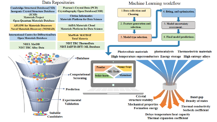
There are several comprehensive materials databases available to researchers those provide access to an extensive list of data for materials, which is essential for the discovery, design, and optimization of new materials. Most of these databases support Application Programming Interface (API) based data retrieval, allowing users to efficiently mine, sort, and, retrieve specific data they need. Web based applications such as aflowlib Curtarolo et al. (2012), JARVIS Choudhary et al. (2020), novel materials discovery laboratory Draxl and Scheffler (2019) (NOMAD) encyclopedia, crystals AI Zheng et al. (2020), citrine informatics (thermoelectric predictor) Gaultois et al. (2016), NIMS tools Tanifuji et al. (2019), SUNCAT Winther et al. (2019) catalysis property predictor, and matlearn Peterson and Brgoch (2021) use advanced ML algorithms and artificial intelligence techniques to predict various properties of materials. These tools can help researchers to screen and design new materials with desirable properties, such as thermoelectric transport properties, electronic structure, catalytic activity, etc. JARVIS, crystals AI, thermoelectric predictor, NIMS tools, SUNCAT, and aflow library are materials simulation software and they use density functional theory (DFT) and ML algorithms to predict properties of materials. Inorganic crystal structure database (ICSD) Belsky et al. (2002), open crystal database (OCD), Pearson crystal structure data (PCXD), and Cambridge Structure Database (CSD) are some of the crystal structure databases those possess experimentally measured crystal structures data of materials. While the open quantum materials database (OQMD) Saal et al. (2013) is a database of quantum mechanical calculations for materials properties. Materials project Jain et al. (2013) is a webbased platform that provides materials data and computational tools for materials scientists and engineers. Citrine informatics is a materials informatics company that uses ML algorithms to analyze and predict material’s properties. Some of the other databases are the materials web online data base Friedman (2009), computational materials repository Rasmussen and Thygesen (2015), materials cloud platform for twodimensional (2D) materials Mounet et al. (2018), Harvard clean energy project (CEP) for organic photovoltaics materials Hachmann et al. (2011), and thermoelectrics design lab for thermoelectric materials Gorai et al. . All these tools and resources are important for materials scientists and engineers to design and discover new materials with desired properties. Each of these web applications specializes in predicting a specific set of material properties and they often include databases of material’s properties those can be used to search for and compare materials with specific properties.
The use of ML has significantly decreased the computational time required for calculating materials properties, as compared to first principles DFT calculations Hohenberg and Kohn (1964); Kohn and Sham (1965). Moreover, this has been achieved without compromising accuracy and has enabled fast descriptive and predictive learning. Further, ML is particularly useful in handling multidimensional data, which is critical for accelerating materials development. Photovoltaics, piezoelectrics, magnetocalorics, magnetoelectrics, and thermoelectrics are some functional materials systems those have benefited from this revolution with demonstrated success in screening and designing efficient materials using ML algorithms. In materials science, selecting the most suitable ML algorithm for a particular application in a specific domain can also be a challenging task. This is because, different algorithms are designed to solve different types of problems and the effectiveness of a particular algorithm can depend on the specific characteristics of the materials data and the features used to train the model. One important consideration when selecting a ML algorithm is the type of materials data that is being analyzed. For example, if the data involves identifying patterns in Xray diffraction spectra or crystallographic data, then ML algorithms such as clustering and pattern recognition may be appropriate. On the other hand, if the data involves predicting mechanical properties or optimizing material processing conditions, then regression and optimization algorithms may be more suitable. If the database has a huge number of data for a specific property then more advanced deep learning techniques may be suitable to employ.
Another factor to consider when selecting a ML algorithm in materials science is the size and complexity of the data. For instance, in the case of highthroughput materials screening, where large volumes of data are generated from diverse materials properties, unsupervised learning algorithms such as principal component analysis (PCA) or clustering may be useful for reducing the dimensionality of the data and identifying important features. Additionally, the desired outcome of the analysis is also a crucial factor in selecting an appropriate ML algorithm. For example, if the goal is to identify new materials with specific properties, then unsupervised learning algorithms such as clustering or generative adversarial networks (GANs) may be more useful Tshitoyan et al. (2019); Jang et al. (2020); Graser et al. (2018); Wei et al. (2019). Finally, the computational resources available and the level of interpretability required are also important considerations when selecting a particular ML algorithm in materials science. Deep learning algorithms such as convolutional neural networks (CNNs) and recurrent neural networks (RNNs) may be more computationally expensive, but they can often provide highly accurate predictions. On the other hand, simpler algorithms such as Decision tree (DT) or Linear regression may be more interpretable and easier to implement. Anyway, whatever model we adopt, the quality of the dataset and appropriate features are key to predict the properties reliably. Here we have adopted regression methods because they are relatively less complex and easy to interpret and evaluate. The motivation behind selectively choosing the models used in this study is their proven superiority in performance on various datasets from diverse fields.
Priyanga et al. Mattur et al. (2022) compared the performance of different ML classifier models for predicting the nature of bandgap. She compared Logistic regression, KNearest Neighbors (KNN), Support vector clustering, Random Forest (RF) Breiman (2001); Liaw et al. (2002); Svetnik et al. (2003); Li et al. (2013), DT Kushwah et al. (2022), Light Gradient Boosting Machine (LGBM) Ke et al. (2017) and eXtreme Gradient Boosting (XGB) Chen and Guestrin (2016); Chen et al. (2015) for their predictability of nature of bandgap for perovskite materials. Wang et al. trained a stacking model Pavlyshenko (2018); Meharie et al. (2022) for bandgap value prediction with LGBM, RF, XGB, and Gradient Boost Decision Tree (GBDT) as base models Wang et al. (2022). Further ML models such as CatBoost Prokhorenkova et al. (2018), Gradient Boosting (GB) Friedman (2001, 2002); Guelman (2012), HistGradientBoosting, ExtraTrees, XGB, DT, bagging Breiman (1996); Bühlmann (2012); Sutton (2005); Friedman and Hall (2007), LGBM, GaussianProcess, artificial neural network (ANN), and light long shortterm memory (LightLSTM) were compared for predictability of photocatalytic degradation of malachite green dye Jaffari et al. (2023). These are few latest studies on material properties using ML models.
The bandgap is a fundamental material property that plays a critical role in different optoelectronic applications. The range of bandgap value required depends on the application and also different materials with varying bandgap values are necessary for various purposes. Materials with a small bandgap value are useful in electronics and detectors, while materials with a large bandgap value are useful in solar cells, LED, and transparent conducting applications. Materials with a narrow bandgap value are useful in thermoelectric devices. Estimating the bandgap value accurately is crucial in Materials Science and can lead to the development of new materials with enhanced properties for various applications, especially, for green energy technologies. Predicting the bandgap value of materials is an important task in Materials Science and has been the subject of many published papers Elsheikh et al. (2014); Radecka et al. (2008); Okumura (2015); Takahashi et al. (2007). To choose the correct model for bandgap prediction, it is important to consider several factors, including the choice of ML algorithm, the quality and size of the dataset, feature selection, model validation, and model interpretability. There are many ML algorithms those can be used for predicting bandgap values, including regression models and neural networks. Each algorithm has its own strengths and weaknesses and the choice of algorithm will depend on the characteristics of the dataset as well as the specific problem being addressed. The quality of the data used to train the model is critical to its accuracy and generalizability.
The another important aspect is that the dataset should be large enough to capture the full range of variability in the material properties and should be representative of the materials being studied to avoid biases. The dataset should also be clean and free of errors or outliers those could skew the predicting capability. The selection of features or inputs those are used to predict bandgap value are important factors in determining the accuracy of the model. Relevant features may include elemental composition, crystal structure, and other material properties. It is important to select features those are relevant to the problem being addressed and that have a strong correlation with the targeted property. Once a model has been trained with the datasets and appropriate features, it is important to validate its performance on a separate test dataset that has not been used for training. This helps to ensure that the model is able to generalize to new data and is not overfitting to the training dataset. The ability to interpret the results of a model is also important for understanding the factors those are driving the predictions. It may be noted that, the models those are more interpretable, such as DT or Linear regression models, can provide insights into the underlying relationships between the input features and the targeted property.
In their study, Heng et al. utilized neural networks and leveraged available experimental data from the literature to predict the bandgap of binary semiconductor alloys Heng et al. (2000). They focused on the elemental properties of the constituents and observed a continuous variation of bandgap values in AiB1-i alloys as the mole fractions of the binary constituents changed. This observation led them to conclude that the bandgap value is influenced by the interplay between attractive and repulsive forces of the constituents as well as the diffusion rate of atoms during the formation of the semiconductor.
Zhuo et al. employed variety of ML methods to model the bandgap energies of 3896 inorganic solids those were reported in experimental studies Zhuo et al. (2018). Their analysis covered a wide range of materials and aimed to accurately predict their bandgap values. By incorporating different ML techniques they sought to improve the understanding and prediction of bandgap values in diverse inorganic solids. Zeng et al. Zeng et al. (2002) extended this analysis to ABC2 type chalcopyrites. They employed neural network techniques to explore the relationship between elemental properties and bandgaps values in this class of materials. By investigating a different class of compounds, they aimed to expand the understanding of the factors influencing bandgap energies. In a different approach, Weston and Stampfl Weston and Stampfl (2018) combined DFT calculations with multiple ML models to predict the bandgap value of Kesterite I2-II-IV-V4 semiconductors. They trained their models using 200 bandgap values calculated using the hybrid HSE functional and focused on classifying these bandgap values as either direct or indirect. This approach allowed them to gain insights into the bandgap characteristics of the Kesterite materials.
These studies collectively demonstrate the application of neural networks, DFT calculations, and ML models in predicting and understanding the bandgap behavior of various semiconductor alloys and inorganic solids. Each study contributed to advancing the knowledge in this field and provided valuable insights into the factors influencing bandgap value and its nature. However, while ML holds enormous potential, it is not a simple process. One of the biggest challenges is collecting and preparing data for analysis. In order to train a ML model, one should first identify the right data sources and ensure that the data is accurate, relevant, and clean. This may involve combining data from multiple sources, such as open databases, literature’s etc and transforming them into a format that can be understood by ML algorithms. Another challenge is selecting the right ML algorithm for a given task. There are many different algorithms to choose from, each with its own strengths and weaknesses. Some algorithms are better suited for classification tasks, while others are better suited for regression tasks. Some algorithms are more robust to noise and outliers, while others are more sensitive to them. Selecting the right algorithm requires careful consideration of the data and the problem at hand. Despite these challenges, ML has become an essential tool for one looking to leverage their data assets and gain a deeper understanding of their task and to accelerate it. By following best practices for data preparation and algorithm selection, one can develop robust and accurate ML models that drive innovation and create new opportunities.
II Data Preparation and Feature Engineering
In this section, we will provide a comprehensive discussion on how to achieve accurate predictions for the bandgap values for HH compounds. We would like to stress the importance of feature engineering in ML methods, as it can significantly affect the predicting capability of the ML models. The selection and engineering of relevant features for a given dataset are crucial for achieving the best possible model accuracy. However, featurizing and selecting specific features with good correlation with targeted properties for a dataset can be a challenging and timeconsuming task. Therefore, we aim to use easily accessible information with the input parameters as simple as possible. We have used the featurization method provided in matminer based on both the composition and structure of the materials, We have used 8 ML models based on the selection of input features, which we will explain in detail in the following sections.
Our objective is to develop appropriate ML models those can accurately predict the bandgap values of large number of HH compound compositions derived based on empirical 18 VEC rule those are expected to be semiconductors, which is essential for identifying new materials with desired bandgap value. We can determine the most effective set of input features for predicting the bandgap values of HH compounds. Through our analysis and discussion, we hope to provide valuable insights into the process of accurately predicting the bandgap values of HH compounds using ML techniques and it can be generalized to predict bandgap values for all inorganic solids. To identify the most relevant features, we used the permutation of features for feature importance and correlation matrix heatmap analysis, which is shown in Fig.2. To assess the performance accuracy of each model, two standard performance metrics were considered and those are RMSE (Root Mean Square Error) and R2 (coefficient of determination). Among these two performance matrices, the R2 metric is a dimensionless statistical measure that indicates how well the data fits a regression line, typically ranging from 0 to 1 and RMSE provides a measure of the average deviation from the actual value. The RMSE expresses the average model predictions in the units (here eV) of the targeted property (here bandgap) used to train the data and is a negatively oriented score, meaning that a lower score indicates better performance of the model. These two performance matrices are defined as.
| (1) |
and
| (2) |
, where yi represents the true value, represents the predicted value, and represents the average value. Additionally, ranges from 1 to N, where N represents the total number of targeted property data present in the test dataset.


To enhance the quality of our feature set, we employed the Pearson correlation method using the pandas library. This technique allowed us to identify features closely related to our targeted property. We then examined a heatmap illustrating the Pearson correlation coefficients (PCC). Only PCC values surpassing the absolute threshold of 0.2 were visualized, as shown in Figure 4(a). These values ranged from -1 to 1, with a higher absolute value indicating a stronger correlation between the target and features. Analyzing the PCC heatmap, we were able to eliminate some features with little or no correlation to the targeted property. For example, a feature with a PCC value close to 0 was likely to be removed, as it would contribute minimally to the model’s predictive ability. Conversely, features with high PCC values were retained, as they were likely to be important predictors of the output variable. The correlation matrix among features as shown in figure2b is also obtained using the Pearson correlation method, which calculates pairwise correlations between features in the columns of a data frame. The resulting correlation values range from -1 to 1, with a higher absolute value signifying a stronger correlation between features. By analyzing the correlation heat map, we effectively eliminated highly correlated features mitigating issues like multicollinearity and overfitting. Through these steps, we reduced the dimensions of our feature space while maintaining its informative aspects.
Our feature selection and processing methods played a crucial role in developing our predictive models. They helped us identify critical features and thus enhance the model’s predictive capacity.

III Machine Learning Algorithm
Composition dependent descriptors are a type of material properties those describe how the properties of a material depend on its composition or the relative amounts of the different elements in the material. One such descriptor is the stoichiometric average of the elemental properties, which is a weighted average of the elemental properties based on their stoichiometry in the material. The stoichiometric average is a useful descriptor because, it takes into account the contributions of all the elements in the material, rather than just one or two dominant elements. The elemental properties those are typically used to calculate the stoichiometric average include the atomic number, ionic radius, electronegativity, and electron configuration of the constituent elements. To calculate the stoichiometric average, the elemental properties are first weighted by their stoichiometric coefficients, which are the numbers those represent the relative amounts of each element in the material. The stoichiometric average can be used to predict the properties of materials based on their composition. For example, it has been found that the stoichiometric average of the electronegativity of the elements in a material can predict its bandgap value if it originates from the ionicity, which is an important property for electronic and optoelectronic applications. Other properties those can be predicted using the stoichiometric average include the thermal and mechanical properties of materials.
We have used the matminer library to obtain a dataset of materials with known bandgap values obtained from GGAPBE calculations and their corresponding composition as well as structure features. In addition to these features, we incorporated the mean, maximum, and standard deviation of atomic numbers as well as the structural features of the corresponding materials by accounting the GGAPBE calculated lattice parameter values , , , , and obtained from the corresponding calculated crystal structure.
We have split the generated dataset into a training set and a testing set with 8:2 ratio. The training set was used to train our models and the testing set was used to evaluate their performance. We have employed the following eight regression models such as RF, GB, XGB, LGBM, DT, AdaBoost Freund et al. (1996); Solomatine and Shrestha (2004); Collins et al. (2002); Shrestha and Solomatine (2006) to identify the best performing model. For the performance analysis, we have considered R2 and RMSE performance metrices to select the best algorithm for our dataset. After assessing the performance of the considered regression models on test data, we found that the RF regressor exhibited the best performance among the considered ML models followed by that the bagging regressor performed well. We have also considered the following seven models as a base for the bagging ensemble model analysis such as DT, CatBoost, GB, LassoCV Tibshirani (1996), LGBM, RidgeCV, XGB With AdaBoost as booster. Among the various models considered in the bagging ensemble model analysis, we found that the bagging with DT and AdaBoost showed the best performance.
The ML regression models were trained using available bandgap values from matminer database obtained from DFT calculations based on GGAPBE functional , excluding the well studied compounds those such as Si, GaAs, TiO2 etc were used for validation. Subsequently, we have performed band structure calculations using the GGAPBE functional to cross validate the ML predicted bandgap value of newly identified HH compounds. Further improve the DFT predicted bandgap value we have also used the TBmBJ functional and the corresponding calculated bandgap values are compared in table4. This combination of ML and DFT hybrid approach holds promising potential for accelerated and reliable bandgap predictions in new semiconducting materials.
| Datasets | ||||
|---|---|---|---|---|
| Model | Dataset(1) 9223 | Dataset(2) 23173 | Dataset(3) 46528 | Dataset(4) 94815 |
| Adaboost | ||||
| 1.252/1.248 | 1.429/1.420 | 1.502/1.493 | 1.536/1.528 | |
| Bagging | ||||
| 0.680/0.306 | 0.662/0.277 | 0.591/0.260 | 0.534/0.235 | |
| CatBoost | ||||
| 0.636/0.385 | 0.634/0.470 | 0.607/0.519 | 0.586/0.530 | |
| LGBM | ||||
| 0.631/0.419 | 0.660/0.535 | 0.657/0.602 | 0.652/0.622 | |
| Random Forest | ||||
| 0.620/0.225 | 0.623/0.226 | 0.563/0.213 | 0.501/0.190 | |
| Decision Tree | ||||
| 0.942/0.0 | 0.860/0.0 | 0.822/0.0 | 0.734/0.0 | |
| GB | ||||
| 0.755/0.697 | 0.833/0.776 | 0.844/0.827 | 0.853/0.844 | |
| XGB | ||||
| 0.635/0.248 | 0.636/0.376 | 0.619/0.462 | 0.587/0.493 | |
IV Results and Discussion
IV.1 Training ML Algorithms to Create an Accurate ML model
The calculation of properties of materials is a complicated and computationally intensive process. The DFT based computational methods are commonly used to calculate almost all the properties of materials. However, when attempting to discover materials with certain desirable properties, this approach can be timeconsuming and computationally expensive. To address this issue, ML approaches based on appropriate features that describe material properties can be developed. Typically in feature engineering, features those strongly correlated with targeted properties are selected while weakly correlated features are ignored in the materials feature set by the feature elimination process. This is because, incorporating weakly correlated features can increase computational complexity and potentially decrease the accuracy of the model. Currently, MLbased materials property prediction mainly relies on composition and geometric structural properties based features. Also, the accuracy of the predicted results heavily rely on the quantity and the quality of the input dataset.
Figure 2 displays a heatmap presenting the PCC values of the most significant features used for training our RF ML regressor such as packing fraction, fraction of valence electrons, transition metal fraction, average of valence electrons, HOMO energy etc. This model is found to be the best performer among the eight stand-alone ML regression models examined in the current study. A comprehensive list of selected features used for these models is provided as supplementary information.
The heatmap shown in Figure 2 was generated for the RF model using the Pearson correlation coefficient (PCC) values obtained from dataset 4. The colors on the heatmap illustrate the correlations between different features. Strong positive correlations are shown with less intense red colors, while strong negative correlations are represented by intense red colors. The diagonal elements are always 1, indicating how each feature correlates with itself. By looking at the correlation heatmap one can identify the important features those are highly correlated. For example, the average number of valence electrons and the fraction of valence electrons in constituent elements in the compound are highly positively correlated. However, the band center and packing fraction have a negative correlation as evident from Fig.2.
Apart from analysing the correlation between features we also analysed the correlation between features and the targeted property. In the heatmap for target property-features correlation shown in Fig.4(a), weak negative correlations are shown in blue colour while shades of red colour represent the strength of positive correlations. Both heatmaps may help in the development of more accurate prediction models by providing insights into the physical mechanisms through various features those determine the bandgap values of materials. A comparison of the performance of 8 ML regression models including AdaBoost, bagging, CatBoost, LGBM, RF, DT, GB, and XGB, with various dataset sizes mentioned in section III are presented in Table1. By comparing different models across various dataset sizes, we have made several observations as follows.
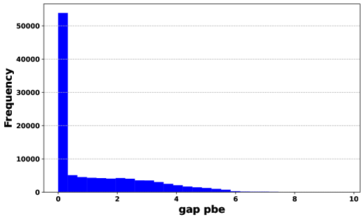
For the performance analysis, we started by examining the AdaBoost regression model. The results indicate that, when tested on 20% of dataset 1, the AdaBoost regression model yielded an value of 0.521 and a RMSE value of 1.252. For the ML model used for the above case we have trained with 80% of dataset 1 for which we obtained and RMSE values of 0.524 and 1.248 eV, respectively. However, as we increased the dataset size, we observed a slight decline in the model’s performance. This is evident from the decreasing values and increasing RMSE values when we trained the ML model with the dataset 2, 3 and 4. This reduced performance is likely attributed to the presence of imbalanced data, which is illustrated in Fig. 4(b). The majority of bandgap values are concentrated between zero and two. It may be noted that the AdaBoost regressor is less adoptable for handling imbalanced data compared to RF and XGB, as discussed earlier Shahri et al. (2021); Krawczyk (2016).
Similarly, we conducted an assessment of the performance of other ML regression models with dataset 1, 2, 3 or 4. This evaluation encompassed an analysis of both RMSE and values for testing as well as training datasets. The outcomes of this evaluation are meticulously presented in Table1. It is worth noting that, the emphasis of this analysis lies in the model’s performance on the test dataset, as it provides insight into the model’s predictive capability on new/unseen data as we done with 20% of unseen data present in the original dataset.
The ML regression models such as Bagging, CatBoost, LGBM, and RF demonstrated competitive performance on both smaller as well as larger dataset sizes. These models consistently displayed high values across various dataset sizes mention in section III. The corresponding decrease in RMSE values indicate that their predictions were highly reliable. This suggests that these regressors can effectively capture the complex relationships between various features with targeted property in smaller datasets and further enhance their performance with the addition of more data. The RF regressor consistently demonstrated high values irrespective of the dataset used and relatively low RMSE values across all dataset sizes considered to train the model in the present study. In the case of dataset 1, the RF model achieved an value of 0.873 and an RMSE of 0.620 eV on testing, indicating its ability to capture a substantial portion of the variance in the targeted property, Moreover, its performance improved further as the dataset size increased. For dataset 4, RF model exhibited the best performance among all the stand-alone models we have analysed here with the R2 and RMSE values 0.943 and 0.501 eV, respectively during testing.
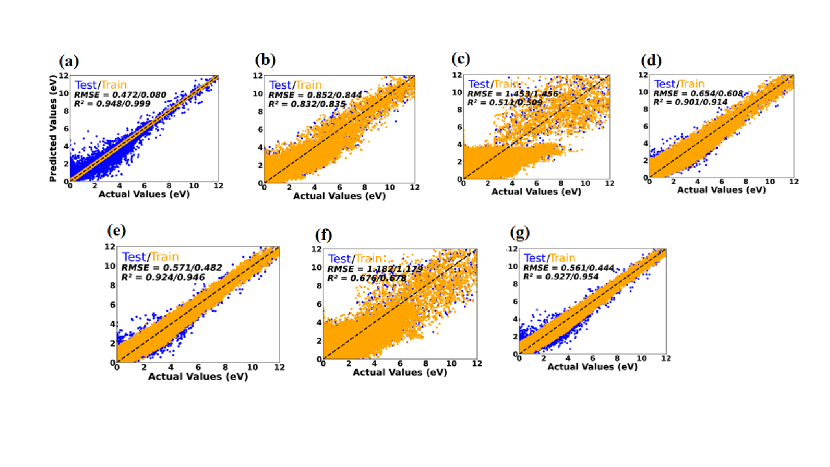
In contrast, the DT regression exhibited limited predictive power when compared to other models. For example, in case of dataset 1, this model achieved an value of 0.729 and an RMSE value of 1.0 eV during the testing, signifying a relatively weak capacity to capture the variance in the targeted property. However, on the training set, it achieved an of 0.942 and an RMSE of 0 eV, implying that the model significantly overfitting to the training data. This inconsistency of DT model performance on the training and testing dataset suggests that it might have overfitted the training data, causing difficulties in generalizing its performance to the test dataset. An important conclusion can be drawn from the above observations that models those are particularly adopt to handle data imbalances and capturing nonlinear relationships between features and also with features and targeted property tend to perform better. Notably, among these models, the RF stands out as particularly well suited for predicting the bandgap values more reliably. The scatter plots for individual models with averaged regression metrics and the predictions corresponding to the training as well as the testing datasets as inputs are shown by orange and blue circles, respectively in Fig. 3.
It is important to additionally consider how a specific model performs on training dataset so that one can evaluate how well it predicts on test data. This enables us to determine the model’s adaptability to various datasets and the presence or absence of overfitting or underfitting, which could have an effect on the algorithm’s performance. When the data points from the training set align exactly with the dashed reference line, this is a sign of overfitting. In this scenario, the algorithm has essentially ”memorized” the training data, which might render it less capable of extrapolating to new and unseen data. Such rigidity could undermine the algorithm’s accuracy/predicting capability for generalised dataset when tasked with predicting bandgap values for previously unencountered materials. Conversely, if the training data points significantly deviate from the dashed line, it points to the presence of underfitting. Underfitting suggests that the algorithm hasn’t fully captured the underlying patterns and complexities as well as nonlinearity of the data, resulting in a less accurate predictive capacity. This situation can lead to sub-optimal performance when applied to new datasets, as the algorithm lacks the capacity to generalize effectively. This means that, a balanced algorithmic performance is needed in both training and testing datasets to reliably predict the properties and obviously for any unseen new data. This balance helps to guarantee that the algorithm can forecast GGAPBE bandgap values for a wide range of materials with high accuracy. The study presented here opens the path for identifying appropriate algorithm for targeted property prediction model development with improved the accuracy.

| Models | R2 | RMSE (eV) |
|---|---|---|
| Test/Train | Test/Train | |
| DT, bagging and AdaBoost | 0.948/0.999 | 0.472/0.080 |
| Catboost, bagging and AdaBoost | 0.924/0.946 | 0.571/0.482 |
| GB, bagging and AdaBoost | 0.832/0.835 | 0.852/0.844 |
| LassoCV, bagging and AdaBoost | 0.511/0.509 | 1.453/1.456 |
| LGBM, bagging and AdaBoost | 0.901/0.914 | 0.654/0.608 |
| RidgeCV, bagging and AdaBoost | 0.676/0.678 | 1.182/1.179 |
| XGB, bagging and AdaBoost | 0.927/0.954 | 0.561/0.444 |
| Models | MetaModels | R2 | RMSE (eV) |
|---|---|---|---|
| Test/Train | Test/Train | ||
| LGBM, RF, XGB | RidgeCV | 0.943/0.991 | 0.494/0.199 |
| RidgeCV, LGBM, RF | LassoCV | 0.942/0.993 | 0.500/0.179 |
| SVR, DT, KNN, | GB | 0.899/0.981 | 0.661/0.286 |
| Linear, RF, GB, | GB | 0.943/0.994 | 0.498/0.166 |
| Composition | Bagging model | Stacking model | GGAPBE | TBmBJ |
|---|---|---|---|---|
| Si | 1.18 | 1.25 | 1.28 Jain et al. (2013) | |
| C | 2.75 | 3.015 | 4.11 Jain et al. (2013) | |
| SiC | 2.09 | 2.03 | 2.30 Jain et al. (2013) | |
| LiF | 7.68 | 8.08 | 8.70 Jain et al. (2013) | |
| BN | 4.70 | 4.532 | 5.77 Jain et al. (2013) | |
| TiO2 | 2.89 | 3.20 | 3.42 Jain et al. (2013) | |
| GaS | 1.743 | 1.70 | 2 Jain et al. (2013) | |
| SiGe | 0.74 | 0.64 | 0.51 Jain et al. (2013) | |
| SiSn | 0.54 | 0.41 | 0.43 Jain et al. (2013) | |
| LuSiAu | 0.10 | 0.07 | 0.33 | 0.43 |
| ScGeAu | 0.13 | 0.12 | 0.13 | 0.56 |
| YCoTe | 0.46 | 0.53 | 0.88 | 1.00 |
| ScSnAu | 0.13 | 0.10 | 0.12 | 0.40 |
| TiGaAg | 0 | 0.01 | 0.2 | 0.11 |
| LaNiBi | 0.20 | 0.20 | 0.34 | 0.55 |
| LuNiSb | 0.19 | 0.16 | 0.18 | 0.19 |
| ZrFeTe | 0.99 | 0.92 | 1.15 | 1.21 |
| ZrSbRh | 0.99 | 0.82 | 1.18 | 1.25 |
| LiZnSb | 0.19 | 0.11 | 0.53 | |
| LuNiAs | 0.15 | 0.12 | 0.45 | 1.37 |
| NbGaNi | 0.05 | 0.02 | 0.047 | 0.15 |
| LaNiSb | 0.12 | 0.23 | 0.45 | |
| LuSbPd | 0.14 | 0.07 | 0.33 | |
| CuSbS2 | 0.81 | 0.78 | 0.72 Jain et al. (2013) | |
| LuSiAg | 0.16 | 0.13 | 0.62 | |
| LiZnAs | 0.32 | 0.43 | 0.35 | 1.37 |
| TiTeOs | 0.33 | 0.368 | 0.45 | 0.96 |
| TiFeTe | 0.67 | 0.77 | 0.98 | 1.2 |
| TiMnO3 | 1.38 | 1.08 | 1.53 Jain et al. (2013) | |
| LiZnP | 1.15 | 1.17 | 1.34 Jain et al. (2013) | |
| LaNiP | 0 | 0.003 | 0 Jain et al. (2013) |
To further improve the performance of our predicting capability of bandgap values through ML approach we have adopted emerging new ML methods such as bagging and stacking approaches. These ensemble ML regression models were utilized to reduce the variance in prediction and average out the predictions of models with similar bias values. A minimum benefit of using ensemble models is the reduction of average prediction spread. These methods are advantageous over 8 different stand-alone ML models used in the present study. Because, these ensemble models combine multiple individual models through a selection strategy, which results in greater generalisability and robustness than adopting a stand-alone ML model Odegua (2019).
The bagging ensemble model, which stands for ”Bootstrap aggregating”, is a robust ensemble learning technique. It operates by dividing the training data into multiple subsets through a process called bootstrapping. Each of these subsets is used as input for individual base models. The results generated by these base models are then combined and fed into the AdaBoost model to produce the final prediction. In essence, bagging creates diversity among the base models and leverages their combined strength. In current study we have taken DT, CatBoost, GB, LassoCV, LGBM, RidgeCV and XGB as the base models and outputs from these base models are then feed into to the AdaBoost model for the final regression.
From our detailed performance analysis we found that the DT taken as base model in bagging and AdaBoost as booster exhibited impressive performance, achieving high values of 0.948 and 0.999 for the test and train datasets, respectively. These results indicate that this model can effectively capture a significant portion of the variance in the targeted property. Furthermore, the corresponding test/train RMSE values of 0.472/0.080 eV suggest that this model’s predictions are relatively close to the actual values with minimal error. The CatBoost as base model in this bagging model also demonstrated very good performance. It achieved R2 values of 0.924/0.946 for the test/train datasets indicating its reliability to predict the bandgap values. This bagging model with Catboost as base accuracy was further validated by the relatively low RMSE values of 0.571/0.482 eV, indicating small prediction errors. The GB as a base model gave an average performance, achieving R2 values of 0.832/0.835 and relatively high RMSE values of 0.852/0.844 eV for the test/train datasets, respectively.


The R2 values for the test and train datasets for the LassoCV as a base model in the bagging regression were just 0.511 and 0.509, respectively. These findings imply that the targeted property’s variation is only moderately explained by the bagging regression with LassoCV as base model. Further, this model’s predicting capability of the targeted property will be relatively poor, as seen by the higher RMSE values of 1.453/1.456 eV for test/train dataset, which represent large prediction errors.
In the bagging model with LassoCV as a base automatically sets coefficients of irrelevant features as zero, leading to loss of information. In contrast, RidgeCV retains all features but shrinks their coefficients simultaneously toward zero Melkumova and Shatskikh (2017). The dropping of features in LassoCV can cause over simplification of the model and results in under fitting the data. If we use the LGBM as base model in our bagging regression, we found that, it gives reasonable performance, achieving R2 values of 0.901/0.914 for the test/train datasets. This suggest that the LassoCV as a base model substantially capture the correlation between features and targeted property i.e, GGAPBE bandgap value here. The corresponding RMSE values of 0.654/0.608 eV for test/train datasets suggest relatively low prediction error compared with that we obtain from LassoCV model. If we use the RidgeCV as base model in our bagging regression, we obtained modest performance with R2 values of 0.676/0.678 for the test/train data-sets. These values suggest that RidgeCV as a base model has moderate ability to capture the correlation between features and the targeted property. Moreover, as the large value of RMSE of 1.182/1.179 eV indicate larger prediction error which suggests that this model is unreliable to predict the targeted property. Finally, the XGB as base model performed well, yielding high R2 values of 0.927/0.954 for the test/train datasets indicating good agreement between predicted and the actual values. The relatively low RMSE values of 0.561/0.444 eV for the test/train datasets further confirm the accuracy of the model to predict the GGAPBE generated bandgap values.
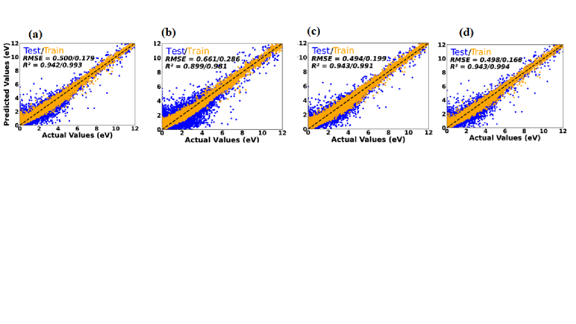
We have also explored the performance of various stacking models by combining different combinations of stand-alone ML regressor models considered in the present study. Among these models, one that stood out used RidgeCV as the meta-model, while employing LGBM, RF, and XGB as the base models. This particular stacking model exhibited promising results, with R2 values of 0.943 and 0.991 for the test and train datasets, respectively. Additionally, this model demonstrated high accuracy, as evidenced by the low RMSE value of 0.494 eV for the test dataset and 0.199 for the train dataset. These RMSE values indicate that this model achieved remarkably small prediction errors, further emphasising its effectiveness.
Similarly, the stacking model consisting of RidgeCV, LGBM, RF as base models and LassoCV as metamodel demonstrated good performance, obtaining R2 values of 0.942/0.993 for the test/train datasets. The corresponding RMSE values of 0.500/0.179 eV for the test/train dataset indicating rather small prediction errors, demonstrating the efficacy of this stacking model. Additionally, the stacking model with SVR, DT, and KNN as base models and GB as the metamodel showed outstanding performance, achieving R2 values of 0.899/0.981 for testing/training dataset. This stacking model’s accuracy was further evidenced by the corresponding smaller RMSE values of 0.661/0.286 eV for the test/train datasets, which showed modest prediction errors. The stacking model where Linear regression, RF, GB are taken as base models and GB as metamodel gave us R2 values of 0.943/0.944 for the test/train datasets, with RMSE values of 0.498/0.166 eV for the test/train datasets, showing modest prediction errors.These results suggest that the stacking models enhance prediction accuracy compared to stand-alone ML models, though to a slightly lesser extent than the bagging models mentioned above.


In Fig.6, scatter plots are shown for above mentioned four different stacking models with averaged regression metrics and the predictions corresponding to the train/test dataset4 where the test and train inputs are shown by orange and blue circles, respectively.
As a measure of comparison for the accuracy of different ML models considered in the present study, the targeted property from the best performing ML models are compared for new compounds those inputs are not considered to train the model. The best performing bagging and stacking model predicted bandgap values are validated using the DFT calculation using VASP code and are compared in Table 4. From this table it is clear that the bandgap values derived from GGAPBE based DFT calculations are in good agreement with predictions of these models.
We would like to emphasise that, further improvements in the predicting capability of these ML models can be achieved by including additional features, new model selection, augment more data etc. Additionally, incorporating domainspecific knowledge and combining ML with physicsbased models, such as DFT, could lead to more reliable and accurate predictions in the future. Upon a more detailed analysis of the results obtaned from ML predictions with those obtained from DFT calculations we have observed several patterns and trends. In general, both the Bagging and Stacking models exhibit a noticeable degree of deviation in predicting the bandgap value obtained from GGAPBE based DFT calculations across various compositions. This indicates that there are inherent complexities and nuances in the dataset those are not adequately captured by the stand-alone ML models.
Among the various ML models considered in the present study, best performing bagging model typically performs better than all stand-alone ML models and the stacking models in terms of predicting the bandgap values close to the computed GGAPBE values for different compositions. For example, in the case of LuSiAu, the bagging model predicts a bandgap value of 0.10 eV, Whereas, the stacking model predicts a value of 0.07 eV. It may be noted that the bandgap prediction from the bagging model is much closer to that from best performing stacking model. However these values are greatly depart from those obtained from GGAPBE value of 0.337 eV in the present study. Moreover, it is important to note that, the deviations between the ML predicted bandgap value and that from GGAPBE vary across different compositions. Some compositions exhibit relatively smaller deviations, indicating a better agreement between the ML models and the calculated bandgap values from DFT calculations as shown in Fig. 7(a). Examples of such compositions include ScGeAu, Si, LiZnP, CuSbS2, TiO2, and SiC. Conversely, compositions such as LuSbPd, LuSiAu, BN, C, and LiZnP demonstrate larger disparities between the bandgap value obtained from ML models and DFT calculations. This indicates that these compositions may possess unique or complex characteristics that are challenging for our trained ML models to capture accurately based on the features we have used to train the model or due to limitations in the dataset used to train our models.
The observed deviations in ML predicted and GGAPBE calculated values highlight the limitations of relying solely on ML techniques for predicting material properties. Even though ML models are powerful in many areas, they struggle with understanding complex quantum effects that greatly impact material properties. These effects are crucial for accurately getting material properties such as bandgap values considered in the present study which can be calculated with reasonable accuracy from DFT calculations. The deviation in the bandgap values between ML predicted and DFT calculated highlight the need to be careful when looking at MLgenerated predictions. While ML can quickly give predictions, it might not fully grasp the intricate quantum behaviors in complex materials. So, it’s wise to be cautious when using ML predictions in situations where being really accurate is important. In a nutshell, comparing the bandgap valued from ML predictions to DFT calculations reminds us that while ML may provide insights, it cannot completely replace the quantum approaches to predict the material properties. Therefore, it is important to keep in mind that we have to employ ML predictions carefully and that they should complement, not replace the more precise quantum approaches. Given the many ways these approaches function to predict the properties of materials the ML approaches may be used to search wide chemical space to identify potential functional materials and followed by that use time consuming quantum approach such as DFT to predict material properties with reasonably accuracy. We believe that such hybrid approaches will be replaced with advanced ML models in future once developed more ML models and more reliable datasets to predict targeted properties.
To improve the predictive accuracy of ML models for material properties, further research and development are necessary. This could involve exploring advanced feature engineering techniques, incorporating additional domain knowledge, and leveraging hybrid approaches that combine ML with DFT/empirical based models. Further, if a model is trained to predict the GGAPBE bandgap values of materials, it is capable to predict GGA bandgap alone for new materials not for bandgap from experimentally or more computationally intensive DFT methods such as GW, hybrid etc. It may be noted that the results obtained from bagging and stacking models still exhibit notable discrepancies compared to calculated DFT values. Continued efforts to refine and enhance these models along with the integration of complementary approaches will be essential to achieve more reliable and accurate predictions in the future.
V Density Functional Theory Calculations
The DFT calculations for structural optimization and the electronic structure calculations were performed using projectoraugmented planewave (PAW) Kresse and Joubert (1999) method, as implemented in the Vienna abinitio simulation package (VASP) Kresse and Furthmüller (1996). The generalized gradient approximation (GGAPBE) Perdew et al. (1996) proposed by PerdewBurke
Ernzerh has been used for the exchangecorrelation potential to compute the equilibrium structural parameters and electronic structure. The irreducible part of the first Brillouin zone (IBZ) was sampled using a Monkhorst pack scheme Monkhorst and Pack (1976) and employed a 121212 kmesh for geometry optimization.
A planewave energy cutoff of 600 eV is used for geometry optimization. The convergence criterion for energy was taken to be 10-6 eV/cell for electronic minimisation step and less than 1 meV/Å is used for HellmannFeynman force acting on each atom to find the equilibrium atomic positions. Our previous study Choudhary and Ravindran (2020) shows that the computational parameters used for the present study are sufficient enough to accurately predict the equilibrium structural parameters for HH compounds. In our electronic structure calculations we focused on the high symmetry directions of the first IBZ of face centered cubic systems. Considering that the GGAPBE method tends to underestimate bandgap values, we have also included results from higher level calculations, such as the TBmBJ method in tablexx though it cannot be compared with ML prediction values. The other theoretical details of these calculations can be found elsewhere Choudhary et al. (2023); Tran and Blaha (2009); Koller et al. (2011, 2012). In order to see the dynamical stability of the predicted four HH alloys based on 18 VEC, we have made lattice dynamic calculation to check for their dynamic stability. The phonon dispersion curves are generated using the finite displacement method implemented in the VASPphonopy Togo and Tanaka (2015) interface with the supercell approach. We have used the relaxed primitive cells to create supercells of dimension 3 × 3 × 3 with the displacement distance of 0.01 Å for our finite displacement calculations to estimate the dynamical matrix.
In Table 4 we have listed out the predicted bandgap values from our ML regression models discussed in section III along with those obtained from DFT calculation mentioned above. It may be noted that, the HH compounds listed in Table 4 are predicted based on 18 VEC rule and their corresponding bandgap values obtained from GGAPBE calculations are directly compared with those predicted from our best performing ML models. This comparison is made to validate our ML trained models performance and also their reliability to predict GGA bandgap value of any unknown new compounds. Additionally, we have predicted the GGAPBE bandgap values for wellstudied compounds such as Si, C, SiC, LiF, BN, TiO2, GaS, SiGe and SiSn (see Fig. 7(a)) using the best performing ML models to show their reliability to predict GGA bandgap value of wide range of semiconductors. The overall observation is that, we have obtained minimal error between the bandgap values calculated using the GGAPBE method and those predicted based on our trained ensemble ML models for well known semiconductors.
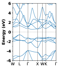
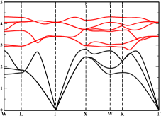
The calculated electronic band structures of newly identified HH compounds ZrFeTe, LuNiSb, ZrSbRh and LaNiBi are displayed in Fig.7 as (a),(b), (c), (d), respectively. From these figures it is clear that all these compounds possess indirect bandgap behavior with the valence band maximum (VBM) located at the point and the conduction band minimum (CBM) at the X point. At the point, the bands near the VBM show a triply degenerate state. The degenerate bands near the VBM create a well dispersed band structure that favors hole conductivity in these systems. However, the flat band dispersion near the CBM along the X direction suggests low electron conductivity due to the high effective mass of electrons.
In order to check the phase stability of our selected compounds, we have made enthalpy of formation () calculations. Our calculated is negative for ZrFeTe, LuNiSb, ZrSbRh and LaNiBi with the value of -0.76 eV/atom, -0.88 eV/atom, -1.0 eV/atom and -0.77 eV/atom, respectively. The negative values confirm that these materials are stable at ambient conditions and also can be synthesised experimentally. Additionally, to check the dynamical stability of those compounds we have calculated the phonon dispersion curves along high symmetry directions within the fcc BZ. We used the Phonopy code with the GGAPBE functional and the finite difference method to compute the phonon dispersion at equilibrium lattice parameters under harmonic approximation. The phonon dispersion curve provides valuable information about the dynamical stability of a crystal. A dynamically stable crystal exhibits only positive (real) phonon frequencies throughout the phonon dispersion curve. In contrast, a dynamically unstable crystal also display negative (imaginary) phonon frequencies. The calculated phonon dispersion curves for predicted new HH alloys are given in Fig.8. From these phonon dispersion curves we found that no one of these compounds exhibit a dynamical instability and hence no negative frequency is found in any of these compounds. This result suggests that all these compounds will be stable under the ambient condition. The observation of high stability in these newly identified HH alloys is consistent with the alloy theory of solids that 18 VEC rule brings extra stability to the system.
VI Conclusions
In summary, our trained best performing machine learning models exhibited minimal deviations from actual values when predicting GGAPBE bandgap values using structural and composition based features. When compared to DFT calculations, ML models trained on existing DFT data can provide comparable prediction accuracy in significantly less time. These ML models can effectively aid in the search for compositions with desirable bandgap value across a wide chemical space, which accelerate material discovery with desired properties. Among the 8 stand-alone ML regression models we have studied, Adaboost performed the poorest. Conversely, the DT model showed signs of over-fitting on the training data, as indicated by its performance matrices. The other stand-alone models consistently improved their performance when we increase the dataset size, emphasising their robustness, accuracy, and generalization capabilities. Notably, CatBoost regression excelled on larger datasets, while LGBM regression demonstrated strong performance on smaller datasets. RF regression consistently delivered reliable results on smaller and mediumsized datasets. GB performed well across datasets of varying sizes, while XGB exhibited mixed performance depending on the dataset size. It is important to note that these results depend on the specific dataset characteristics, feature engineering techniques, and preprocessing steps used. More exploration and experimentation with different combinations of features and preprocessing techniques can further enhance the predictive capabilities of these models.
The selection of an appropriate model should be based on a comprehensive understanding of the dataset and the specific requirements of the prediction task. Subsequently, we employed above mentioned stand alone ML models to predict the bandgap values of new HH compounds designed based on 18 VEC. Through this process, we identified several new materials with significant potential for applications in thermoelectrics, solar cells, and photocatalysis. In addition, we employed ensemble model such as stacking and bagging models to enhance the predicting capability for obtaining the GGAPBE bandgap values for unseen datasets. It’s important to take into account that in this study, we adopted GGAPBE bandgap values to train our ML models. For attaining a superior level of accuracy to predict the bandgap value on par with that measured experimentally, we have to train our ML models with experimental bandgap values which is available only for very limited number of systems. Also, the best performing ML models can be trained using the bandgap values obtained from more advanced DFT calculations such as hybrid functionals, GW method etc. However the bandgap values obtained from such advanced DFT methods are very limited owing to the fact that such calculation are computationally very intensive. Moreover, the calculated phonon dispersion curve and negative in all the selected compounds considered in this study confirmed their phase and dynamic stability at ambient condition. We hope that the present approach hold the potential to greatly expedite the discovery of new materials possessing desirable properties for various energyrelated applications.
VII Conflicts of interest
There are no conflicts to declare.
Acknowledgements
The authors are grateful to the SCANMAT Centre, Central University of Tamil Nadu, Thiruvarur for providing the computer time at the SCANMAT supercomputing facility. The authors would also like to acknowledge the SERBCore Research Grant (CRG) vide file no.CRG/2020/001399.
References
- Ward et al. (2018) L. Ward, A. Dunn, A. Faghaninia, N. E. Zimmermann, S. Bajaj, Q. Wang, J. Montoya, J. Chen, K. Bystrom, M. Dylla, et al., Computational Materials Science 152, 60 (2018).
- Sarker (2021) I. H. Sarker, SN computer science 2, 160 (2021).
- (3) .
- Lee and Lim (2021) C. Lee and C. Lim, Technological Forecasting and Social Change 167, 120653 (2021).
- Ahmad et al. (2022) T. Ahmad, R. Madonski, D. Zhang, C. Huang, and A. Mujeeb, Renewable and Sustainable Energy Reviews 160, 112128 (2022).
- Guan et al. (2020) C. Guan, J. Mou, and Z. Jiang, International Journal of Innovation Studies 4, 134 (2020).
- Esmaeilzadeh (2020) P. Esmaeilzadeh, BMC medical informatics and decision making 20, 1 (2020).
- Reddy et al. (2020) S. Reddy, S. Allan, S. Coghlan, and P. Cooper, Journal of the American Medical Informatics Association 27, 491 (2020).
- Bishara et al. (2023) D. Bishara, Y. Xie, W. K. Liu, and S. Li, Archives of computational methods in engineering 30, 191 (2023).
- Panchal et al. (2019) J. H. Panchal, M. Fuge, Y. Liu, S. Missoum, and C. Tucker, Journal of Mechanical Design 141 (2019).
- Ramprasad et al. (2017) R. Ramprasad, R. Batra, G. Pilania, A. Mannodi-Kanakkithodi, and C. Kim, npj Computational Materials 3, 54 (2017).
- Lee et al. (2016) J. Lee, A. Seko, K. Shitara, K. Nakayama, and I. Tanaka, Physical Review B 93, 115104 (2016).
- Oliynyk et al. (2016) A. O. Oliynyk, E. Antono, T. D. Sparks, L. Ghadbeigi, M. W. Gaultois, B. Meredig, and A. Mar, Chemistry of Materials 28, 7324 (2016).
- Butler et al. (2018) K. T. Butler, D. W. Davies, H. Cartwright, O. Isayev, and A. Walsh, Nature 559, 547 (2018).
- Morgan and Jacobs (2020) D. Morgan and R. Jacobs, Annual Review of Materials Research 50, 71 (2020).
- Suh et al. (2020) C. Suh, C. Fare, J. A. Warren, and E. O. Pyzer-Knapp, Annual Review of Materials Research 50, 1 (2020).
- Liu et al. (2017) Y. Liu, T. Zhao, W. Ju, and S. Shi, Journal of Materiomics 3, 159 (2017).
- Juan et al. (2021) Y. Juan, Y. Dai, Y. Yang, and J. Zhang, Journal of Materials Science & Technology 79, 178 (2021).
- Cole (2020) J. M. Cole, Accounts of chemical research 53, 599 (2020).
- Oganov et al. (2019) A. R. Oganov, C. J. Pickard, Q. Zhu, and R. J. Needs, Nature Reviews Materials 4, 331 (2019).
- Pulido et al. (2017) A. Pulido, L. Chen, T. Kaczorowski, D. Holden, M. A. Little, S. Y. Chong, B. J. Slater, D. P. McMahon, B. Bonillo, C. J. Stackhouse, et al., Nature 543, 657 (2017).
- Curtarolo et al. (2012) S. Curtarolo, W. Setyawan, S. Wang, J. Xue, K. Yang, R. H. Taylor, L. J. Nelson, G. L. Hart, S. Sanvito, M. Buongiorno-Nardelli, et al., Computational Materials Science 58, 227 (2012).
- Choudhary et al. (2020) K. Choudhary, K. F. Garrity, A. C. Reid, B. DeCost, A. J. Biacchi, A. R. Hight Walker, Z. Trautt, J. Hattrick-Simpers, A. G. Kusne, A. Centrone, et al., npj computational materials 6, 173 (2020).
- Draxl and Scheffler (2019) C. Draxl and M. Scheffler, Journal of Physics: Materials 2, 036001 (2019).
- Zheng et al. (2020) C. Zheng, C. Chen, Y. Chen, and S. P. Ong, Patterns 1, 100013 (2020).
- Gaultois et al. (2016) M. W. Gaultois, A. O. Oliynyk, A. Mar, T. D. Sparks, G. J. Mulholland, and B. Meredig, Apl Materials 4, 053213 (2016).
- Tanifuji et al. (2019) M. Tanifuji, A. Matsuda, and H. Yoshikawa, in 2019 8th International Congress on Advanced Applied Informatics (IIAI-AAI) (IEEE, 2019) pp. 1021–1022.
- Winther et al. (2019) K. T. Winther, M. J. Hoffmann, J. R. Boes, O. Mamun, M. Bajdich, and T. Bligaard, Scientific data 6, 75 (2019).
- Peterson and Brgoch (2021) G. G. Peterson and J. Brgoch, Journal of Physics: Energy 3, 022002 (2021).
- Belsky et al. (2002) A. Belsky, M. Hellenbrandt, V. L. Karen, and P. Luksch, Acta Crystallographica Section B: Structural Science 58, 364 (2002).
- Saal et al. (2013) J. E. Saal, S. Kirklin, M. Aykol, B. Meredig, and C. Wolverton, Jom 65, 1501 (2013).
- Jain et al. (2013) A. Jain, S. P. Ong, G. Hautier, W. Chen, W. D. Richards, S. Dacek, S. Cholia, D. Gunter, D. Skinner, G. Ceder, et al., APL materials 1, 011002 (2013).
- Friedman (2009) G. L. Friedman, ELT journal 63, 126 (2009).
- Rasmussen and Thygesen (2015) F. A. Rasmussen and K. S. Thygesen, The Journal of Physical Chemistry C 119, 13169 (2015).
- Mounet et al. (2018) N. Mounet, M. Gibertini, P. Schwaller, D. Campi, A. Merkys, A. Marrazzo, T. Sohier, I. E. Castelli, A. Cepellotti, G. Pizzi, et al., Nature nanotechnology 13, 246 (2018).
- Hachmann et al. (2011) J. Hachmann, R. Olivares-Amaya, S. Atahan-Evrenk, C. Amador-Bedolla, R. S. Sánchez-Carrera, A. Gold-Parker, L. Vogt, A. M. Brockway, and A. Aspuru-Guzik, The Journal of Physical Chemistry Letters 2, 2241 (2011).
- (37) P. Gorai, D. Gao, B. Ortiz, S. Miller, S. A. Barnett, T. Mason, Q. Lv, V. Stevanović, and E. S. Toberer, .
- Hohenberg and Kohn (1964) P. Hohenberg and W. Kohn, Physical review 136, B864 (1964).
- Kohn and Sham (1965) W. Kohn and L. J. Sham, Physical review 140, A1133 (1965).
- Tshitoyan et al. (2019) V. Tshitoyan, J. Dagdelen, L. Weston, A. Dunn, Z. Rong, O. Kononova, K. A. Persson, G. Ceder, and A. Jain, Nature 571, 95 (2019).
- Jang et al. (2020) J. Jang, G. H. Gu, J. Noh, J. Kim, and Y. Jung, Journal of the American Chemical Society 142, 18836 (2020).
- Graser et al. (2018) J. Graser, S. K. Kauwe, and T. D. Sparks, Chemistry of Materials 30, 3601 (2018).
- Wei et al. (2019) J. Wei, X. Chu, X.-Y. Sun, K. Xu, H.-X. Deng, J. Chen, Z. Wei, and M. Lei, InfoMat 1, 338 (2019).
- Mattur et al. (2022) M. N. Mattur, N. Nagappan, S. Rath, T. Thomas, et al., Journal of Materiomics 8, 937 (2022).
- Breiman (2001) L. Breiman, Machine learning 45, 5 (2001).
- Liaw et al. (2002) A. Liaw, M. Wiener, et al., R news 2, 18 (2002).
- Svetnik et al. (2003) V. Svetnik, A. Liaw, C. Tong, J. C. Culberson, R. P. Sheridan, and B. P. Feuston, Journal of chemical information and computer sciences 43, 1947 (2003).
- Li et al. (2013) X. Li et al., Chinese Journal of Applied Entomology 50, 1190 (2013).
- Kushwah et al. (2022) J. S. Kushwah, A. Kumar, S. Patel, R. Soni, A. Gawande, and S. Gupta, Materials Today: Proceedings 56, 3571 (2022).
- Ke et al. (2017) G. Ke, Q. Meng, T. Finley, T. Wang, W. Chen, W. Ma, Q. Ye, and T.-Y. Liu, Advances in neural information processing systems 30 (2017).
- Chen and Guestrin (2016) T. Chen and C. Guestrin, in Proceedings of the 22nd acm sigkdd international conference on knowledge discovery and data mining (2016) pp. 785–794.
- Chen et al. (2015) T. Chen, T. He, M. Benesty, V. Khotilovich, Y. Tang, H. Cho, K. Chen, R. Mitchell, I. Cano, T. Zhou, et al., R package version 0.4-2 1, 1 (2015).
- Pavlyshenko (2018) B. Pavlyshenko, in 2018 IEEE Second International Conference on Data Stream Mining & Processing (DSMP) (IEEE, 2018) pp. 255–258.
- Meharie et al. (2022) M. G. Meharie, W. J. Mengesha, Z. A. Gariy, and R. N. Mutuku, Engineering, Construction and Architectural Management 29, 2836 (2022).
- Wang et al. (2022) T. Wang, K. Zhang, J. Thé, and H. Yu, Computational Materials Science 201, 110899 (2022).
- Prokhorenkova et al. (2018) L. Prokhorenkova, G. Gusev, A. Vorobev, A. V. Dorogush, and A. Gulin, Advances in neural information processing systems 31 (2018).
- Friedman (2001) J. H. Friedman, Annals of statistics , 1189 (2001).
- Friedman (2002) J. H. Friedman, Computational statistics & data analysis 38, 367 (2002).
- Guelman (2012) L. Guelman, Expert Systems with Applications 39, 3659 (2012).
- Breiman (1996) L. Breiman, Machine learning 24, 123 (1996).
- Bühlmann (2012) P. Bühlmann, Bagging, boosting and ensemble methods (Springer, 2012).
- Sutton (2005) C. D. Sutton, Handbook of statistics 24, 303 (2005).
- Friedman and Hall (2007) J. H. Friedman and P. Hall, Journal of statistical planning and inference 137, 669 (2007).
- Jaffari et al. (2023) Z. H. Jaffari, A. Abbas, S.-M. Lam, S. Park, K. Chon, E.-S. Kim, and K. H. Cho, Journal of Hazardous Materials 442, 130031 (2023).
- Elsheikh et al. (2014) M. H. Elsheikh, D. A. Shnawah, M. F. M. Sabri, S. B. M. Said, M. H. Hassan, M. B. A. Bashir, and M. Mohamad, Renewable and sustainable energy reviews 30, 337 (2014).
- Radecka et al. (2008) M. Radecka, M. Rekas, A. Trenczek-Zajac, and K. Zakrzewska, Journal of power sources 181, 46 (2008).
- Okumura (2015) H. Okumura, Mrs Bulletin 40, 439 (2015).
- Takahashi et al. (2007) K. Takahashi, A. Yoshikawa, and A. Sandhu, Verlag Berlin Heidelberg (2007).
- Heng et al. (2000) K. L. Heng, S. J. Chua, and P. Wu, Chemistry of materials 12, 1648 (2000).
- Zhuo et al. (2018) Y. Zhuo, A. Mansouri Tehrani, and J. Brgoch, The journal of physical chemistry letters 9, 1668 (2018).
- Zeng et al. (2002) Y. Zeng, S. J. Chua, and P. Wu, Chemistry of materials 14, 2989 (2002).
- Weston and Stampfl (2018) L. Weston and C. Stampfl, Physical Review Materials 2, 085407 (2018).
- Freund et al. (1996) Y. Freund, R. E. Schapire, et al., in icml, Vol. 96 (Citeseer, 1996) pp. 148–156.
- Solomatine and Shrestha (2004) D. P. Solomatine and D. L. Shrestha, in 2004 IEEE International Joint Conference on Neural Networks (IEEE Cat. No. 04CH37541), Vol. 2 (IEEE, 2004) pp. 1163–1168.
- Collins et al. (2002) M. Collins, R. E. Schapire, and Y. Singer, Machine Learning 48, 253 (2002).
- Shrestha and Solomatine (2006) D. L. Shrestha and D. P. Solomatine, Neural computation 18, 1678 (2006).
- Tibshirani (1996) R. Tibshirani, Journal of the Royal Statistical Society Series B: Statistical Methodology 58, 267 (1996).
- Shahri et al. (2021) N. Shahri, S. B. S. Lai, M. B. Mohamad, H. Rahman, and A. B. Rambli, Math Stat 9, 379 (2021).
- Krawczyk (2016) B. Krawczyk, Progress in Artificial Intelligence 5, 221 (2016).
- Odegua (2019) R. Odegua, in Proc. Conf.: Deep Learn. IndabaXAt (2019).
- Melkumova and Shatskikh (2017) L. Melkumova and S. Y. Shatskikh, Procedia engineering 201, 746 (2017).
- Kresse and Joubert (1999) G. Kresse and D. Joubert, Physical review b 59, 1758 (1999).
- Kresse and Furthmüller (1996) G. Kresse and J. Furthmüller, Computational materials science 6, 15 (1996).
- Perdew et al. (1996) J. P. Perdew, K. Burke, and M. Ernzerhof, Physical review letters 77, 3865 (1996).
- Monkhorst and Pack (1976) H. J. Monkhorst and J. D. Pack, Physical review B 13, 5188 (1976).
- Choudhary and Ravindran (2020) M. K. Choudhary and P. Ravindran, Sustainable Energy & Fuels 4, 895 (2020).
- Choudhary et al. (2023) M. K. Choudhary, H. Fjellvåg, and P. Ravindran, Computational Materials Science 216, 111856 (2023).
- Tran and Blaha (2009) F. Tran and P. Blaha, Physical review letters 102, 226401 (2009).
- Koller et al. (2011) D. Koller, F. Tran, and P. Blaha, Physical Review B 83, 195134 (2011).
- Koller et al. (2012) D. Koller, F. Tran, and P. Blaha, Physical Review B 85, 155109 (2012).
- Togo and Tanaka (2015) A. Togo and I. Tanaka, Scripta Materialia 108, 1 (2015).