Composite pulses for high fidelity population transfer in three-level systems
Abstract
In this work, we propose a composite pulses scheme by modulating phases to achieve high fidelity population transfer in three-level systems. To circumvent the obstacle that not enough variables are exploited to eliminate the systematic errors in the transition probability, we put forward a cost function to find the optimal value. The cost function is independently constructed either in ensuring an accurate population of the target state, or in suppressing the population of the leakage state, or both of them. The results demonstrate that population transfer is implemented with high fidelity even when existing the deviations in the coupling coefficients. Furthermore, our composite pulses scheme can be extensible to arbitrarily long pulse sequences. As an example, we employ the composite pulses sequence for achieving the three-atom singlet state in an atom-cavity system with ultrahigh fidelity. The final singlet state shows robustness against deviations and is not seriously affected by waveform distortions. Also, the singlet state maintains a high fidelity under the decoherence environment.
I Introduction
Implementation of high fidelity quantum coherent control is a top priority in quantum information processing (QIP) Salières et al. (1995); Bergmann et al. (1998); Makhlin et al. (2001); Zhao et al. (2006); McCullough et al. (2000); Gordon et al. (2002); Zeng et al. (2020); Devolder et al. (2021); Levine et al. (2018); Daems et al. (2013). Many works Allen and Eberly (1975); Vitanov et al. (2001); Guéry-Odelin et al. (2019), which design different kinds of pulse shapes, have been devoted to ensuring a remarkable quantum computing performance. Originally, the resonant pulse (RP) technique, where the frequency of radiation exactly matches the transition frequency, is regarded as a popular tool to accurately achieve coherent control, due to its fast operation and simple waveform Scully and Zubairy (1997). For example, one can achieve complete population inversion through a -pulse, or a maximum superposition state through a -pulse Gerry and Knight (2004). However, the resonant pulse is extremely susceptible to external perturbations, such as fluctuations of control fields. To overcome this difficulty, the adiabatic passage (AP) technique has been developed Shankar (1994); Král et al. (2007). The AP technique selects one eigenstate of the system Hamiltonian as an evolution path and propels the initial state to adiabatically evolve along this path. In this technique, the robustness against parameter perturbations is improved at the cost of the slow evolution rate and lower fidelity. To enjoy both the ultrahigh fidelity of RP and the robustness of AP, one can adopt the composite pulses (CPs) technique.
The CPs technique, comprised of a well-organized train of constant pulses with determined pulse areas and relative phases, was conceived in early nuclear magnetic resonance (NMR) Wimperis (1991, 1994); Levitt and Freeman (1979); Levitt (1986). To date, this technique has been used extensively in QIP Brown et al. (2004); Dridi et al. (2020); Torosov and Vitanov (2011); Genov et al. (2014); Torosov and Vitanov (2018); Jones (2013); Vitanov (2011); Torosov and Vitanov (2019a); Torosov et al. (2020a); Genov et al. (2020). One unique feature of CPs is that the pulse sequence is available to compensate for the systematic error in any physical parameters (e.g., pulse duration, pulse amplitude, detuning, Stark shift, etc.) Genov et al. (2014); Brown et al. (2004); Levitt (1986); Dridi et al. (2020); Torosov and Vitanov (2011). Previous works Torosov et al. (2015); Ichikawa et al. (2011); Cohen et al. (2016); Kyoseva et al. (2019); Wang et al. (2014); Mount et al. (2015); Demeter (2016) about precise quantum control are mostly based on two-level systems. For example, by using a narrow-band composite sequence of laser pulses, the error-tolerance region of high fidelity local addressing operation in trapped ions and atoms is improved by Ivanov and Vitanov (2011). Besides, an arbitrary single-qubit gate, which is robust against pulse area error, could be implemented by a composite pulses sequence Torosov and Vitanov (2019b).
At present, works on CPs in two-level systems are relatively complete and extensive Vandersypen and Chuang (2005). As is well known, the three-level system is another representative physical model in QIP. Some interesting phenomena, such as coherent trapping Scully and Zubairy (1997), electromagnetically induced transparency Fleischhauer et al. (2005), and lasing without inversion Scully et al. (1989) manifest in three-level systems. Recently, works on a general use of CPs scheme in three-level systems are still deficient Levitt et al. (1984); Ramamoorthy and Narasimhan (1991); Torosov et al. (2011); Torosov and Vitanov (2013); Schraft et al. (2013); Ishida et al. (2018). The main difficulty is that the analytical expression of the propagator is very complicated for a general three-level system. One way to deal with this difficulty is to reduce the three-level system into one or more two-level systems. In Ref. Torosov et al. (2020b), the closed-loop three-level system of the chiral molecule is divided into three independent two-level systems Lehmann (2018); Leibscher et al. (2019). Then, the CPs sequence using RP in these two-level systems achieves the chiral resolution necessary to overcome Rabi frequency errors and detuning errors. In Refs. Genov et al. (2011); Torosov and Vitanov (2020), two powerful tools, Morris-Shore transformation Morris and Shore (1983) and Majorana decomposition Majorana (1932), are exploited to simplify a three-level system into an effective two-level system, so as to obtain the propagator of the system. Note that some approximations or restrictions are usually adopted in this simplification process. Specifically, Morris-Shore transformation Morris and Shore (1983) is applied when the system can be mapped into two sets of states with the same energies (in the rotating-wave approximation) and two coupling coefficients must have the same time dependence, while Majorana decomposition Majorana (1932) always demands that the system have the SU(2) dynamic symmetry. The common feature of these approaches Genov et al. (2011); Torosov and Vitanov (2020); Morris and Shore (1983); Majorana (1932) is to reduce the dynamics of the three-level system to a two-level system dynamics. As a result, one ignores the dynamics of the excited (leakage) state and thus the system does not exist the population leakage. However, the dynamics of the excited state should be considered in the three-level system, and that is what makes a three-level system different from a two-level system. It is therefore necessary to conceive a general CPs sequence able to directly achieve precise and robust control in a three-level system.
In three-level systems, there are some issues that must be considered. For instance, during the construction process of qubits, the existence of the leakage state, which is beyond the computational subspace, leads to an imperfect quantum operation performance. This issue is inevitable and poses a great threat to the fidelity of qubit operations. The works on suppressing leakage in three-level systems are ongoing Ghosh et al. (2017); Shi et al. (2021). Besides, compared to the two-level system, the additional modulation parameters in the three-level system may lead to various types of systematic errors. The existence of these systematic errors has a detrimental effect on the quantum operation accuracies, to various degrees. On the other hand, as shown in Refs. Genov et al. (2014); Torosov and Vitanov (2011, 2018); Dridi et al. (2020), the fidelity improves with the increase in the number of pulses. However, considering the finite coherence time, a large number of pulses would cost long evolution time, which is tremendously detrimental for quantum computation. Therefore, one generally requires the number of pulses to be as small as possible, hence it is essential to learn how to efficiently eliminate the systematic errors within finite pulses. This is especially true in the case where the quantum systems have various types of deviations.
In this work, we achieve arbitrary population transfer by phase modulation CPs in the three-level system. We directly deduce the transition probability of each state, including the excited state. In other words, we concern the dynamics of the excited state as well. By using the Taylor expansion, the transition probability of the target (leakage) state can be sorted by different order derivatives. Then, we construct a cost function to overcome the difficulty that there are not enough variables to eliminate high-order derivatives in the short pulse sequence. Different cost functions have respective purposes for accurately controlling population transfer or effectively suppressing population leakage, or both of them. We study minutely two kinds of short pulse sequences as examples to demonstrate the pulse design process, which can easily extend to longer pulse sequences. For applications, our CPs scheme further shows the feasibility of achieving the three-atoms singlet state with ultrahigh fidelity in an atoms-cavity system. The results indicate that the final singlet state is robust against several kinds of defects, including deviations in coupling coefficients, waveform distortions, and the disturbances of the decoherence environment.
The paper is organized as follows. In Sec. II, we design the CPs sequence in the three-level system through minimizing the cost function. In Sec. III, we first employ different cost functions to analytically search for the best group of phases in the two-pulse sequence. For more than two pulses, we adopt numerical methods to find different phases of the CPs sequence. In principle, the numerical methods are suitable for arbitrary long pulse sequences. In Sec. IV, we study the feasibility of the CPs sequence through a specific application in the atom-cavity system. Finally, a conclusion is given in Sec. V.
II Toy model and the general theory
Consider a -type three-level quantum system interacting with two external fields, where the three-level system has two ground states and , and an excited state . The ground states and , acting as a qubit, cannot be immediately coupled to each other. Hence, we require an extra excited state to construct the indirect coupling between two ground states. More specifically, the transition () is driven by the external field with the coupling strength (), the phase (), and the detuning . In presence of deviations in the external fields, in the interaction picture, the system Hamiltonian is given by ()
| (1) |
where the deviations and are random unknown constants, which would give rise to the systematic errors during quantum operations.
Here, we do not intend to specify a concrete physical system, because the three-level system studied here can be found in very different physics research fields ranging from high precision spectroscopy, to quantum information processing, NMR, and metrology. For example, this physical model is quite familiar in the quantum system of a three-level atom interacting with two laser fields Scully and Zubairy (1997). In the atomic system, the inhomogeneous distribution of the laser fields leads to different interaction coefficients between the atom and the laser fields. Also, the spatial position of the atom cannot be exactly determined due to its micro-vibration. As a result, the interaction coefficients in the system are susceptible to deviations. It is worth mentioning that similar energy-level structures can also be found in trapped ions Leibfried et al. (2003), diamond nitrogen-vacancy centers Yang et al. (2010), and superconducting circuits Xiang et al. (2013); Xue et al. (2017); Kang et al. (2016, 2017); Hong et al. (2018); Chen et al. (2020). In addition, some complicated quantum systems, such as the electrons in semiconductors Greentree et al. (2004), the spin chain Bruderer et al. (2012); Chen and Li (2016), neutral atoms interactions Li and Shao (2018); Kang et al. (2018); Shi et al. (2018); Li et al. (2020); Shao (2020); Wu et al. (2021), and massive quantum particles in an optical Lieb lattice Taie et al. (2020), can be reduced to the three-level physical model as well.
Assume that the system is initially in the ground state . If there are no deviations in the external fields (i.e., and ), one can easily achieve perfect population transfer for the qubit. To this end, we choose the evolution time , then the population of the ground state becomes
| (2) |
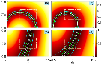
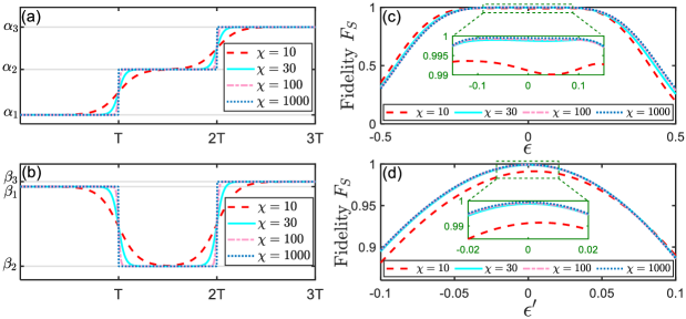
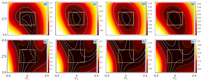
Thus, the value of can be modulated by altering either the detuning or the ratio of two coupling coefficients. However, in presence of deviations in the external fields, the actual population would keep away from the desired value . This is verified in Figs. 1(a) and 1(c), which demonstrate that the infidelity is high even for small deviations. Note that Figs. 1(a) and 1(c) also demonstrate that the value of infidelity becomes extremely low in some regions where the deviations are large, e.g., when and in Fig. 1(c). However, it is meaningless in practice, because the values of the deviations and are unknown in principle and they are usually independent of each other. On the other hand, population leakage from the ground states to the excited state invariably does happen in the presence of deviations, which can be observed in Figs. 1(b) and 1(d). Hence, the goal of this work is to precisely achieve the predefined population , and meanwhile, to dramatically suppress the population leakage by designing a composite -pulse sequence.
First, we require to calculate the population of the ground state in absence of the deviations. Assume that the Hamiltonian of the th pulse has the following form ()
| (3) | |||||
For the pulse duration , the corresponding propagator, labelled as , can be written as (up to a global phase)
| (7) |
where
Then, the total propagator of the composite -pulse sequence can be written as
The detailed derivation of the total propagator is given in Appendix A. After some algebraic manipulations, the population of the ground state , labelled as , becomes
| (8) |
where the expression of is also presented in Appendix A. For simplicity, we set in the following, which means that the three-level system works in the resonant regime. Apparently, the following analysis can be easily generalized to the two-photon resonant regime. Furthermore, we choose (), which means that two coupling coefficients and remain unchanged in the -pulse sequence. Note that it is also suitable for the other values of . As a result, we only modulate the phases and , and the form of CPs now becomes
In presence of deviations in the external fields, by the Taylor expansion, the actual population of the ground state can be written as
| (9) | |||||
where () are the coefficients of the th-order term in the -pulse sequence. To achieve the predefined population , one should design the phases and () to guarantee the validity of the following equation
| (10) |
That is, the zeroth-order term of the actual population should be equal to the predefined population. This is the first condition that the phases and must satisfy. Furthermore, the global phase of the propagator is inessential for the system dynamics, and what really matters is the phase difference and (). Hence, one can set the phases and of the first pulse to be arbitrary. Nevertheless, they become extremely useful when the composite pulses are designed for single qubit gates, because the values of and can be used to modulate the relative phase between the ground states. As a result, apart from Eq. (10), there still remain free phases (variables) in the -pulse sequence, which can be designed to compensate for the systematic errors caused by the deviations and .
Unlike the case of two-level systems Torosov et al. (2020a); Genov et al. (2020); Torosov et al. (2015); Ichikawa et al. (2011); Cohen et al. (2016); Kyoseva et al. (2019); Wang et al. (2014); Mount et al. (2015); Demeter (2016), there exists a population leakage from the ground states to the excited state in the three-level system. Thus, we need to suppress population leakage (i.e., the population of the excited state ) as well. Similar to the treatment of , the actual population of the excited state can be expanded by the Taylor expansion, as follows
| (11) | |||||
where () are the coefficients of the th-order term in the -pulse sequence. Contrary to Eq. (9), Eq. (11) does not contain the first-order term.
Therefore, to obtain high fidelity population transfer in the qubit, the general method is to satisfy the following conditions: () eliminate the higher-order terms in as much as possible. Namely, ; () demand that the value of be as small as possible, i.e., . Note that the design procedure of the phases is more complicated in three-level systems than that in two-level systems Torosov et al. (2020a); Genov et al. (2020); Torosov et al. (2015); Ichikawa et al. (2011); Cohen et al. (2016); Kyoseva et al. (2019); Wang et al. (2014); Mount et al. (2015); Demeter (2016), since there are two coefficients [ and ] in the first-order term while there are six coefficients [ and , ] in the second-order term, and so forth. Particularly, when considering the small number of pulses, which is often the practical case, it does not have sufficient phases to eliminate the systematic errors up to the desired order.
To solve this issue, we can proceed as follows. First, it is worth noting that the influence of the higher-order term of systematic errors on dynamical evolution would gradually diminish. Therefore, the first-order terms have the most serious effect on dynamical evolution, and we should give priority to making these terms vanish by designing suitable phases, i.e., . Then, the remaining phases are designed to minimize the following cost function:
| (12) | |||||
| (13) | |||||
| (14) |
where and are the weighting coefficients, satisfying and . Physically, the cost function represents the trade-off between the accuracy of population transfer and the leakage to the excited state . The conditions and ensure that the coefficients of the low order terms have a high weight, and thus are preferentially eliminated. Remarkably, different weighting coefficients have different effects. Setting , we have the cost function aimed to keep the accuracy of the population transfer, while setting we have the cost function aimed to reduce the leakage to the excited state . Note that the minimum value of the cost function is zero, corresponding to satisfy the equations: .
III Robust implementation of arbitrary population transfer by composite pulses
In this section, we present the design process of the phases and () to achieve high fidelity population transfer by the -pulse sequence. For the two-pulse sequence, the phases are derived analytically, while for the three-pulse sequence we combine both the analytical method and the numerical method to obtain the phases. For more than three pulses, we carry out the four(five)-pulse sequence by numerical calculations to demonstrate the feasibility of eliminating the higher-order terms of the systematic errors. It is worth mentioning that the cycle of the phases is , thus we restrict the values of all phases in the interval following from here.
III.1 Two pulses
The form of the two-pulse sequence is expressed by
and the zeroth-order coefficient in Eq. (9) becomes
| (15) |
where and . As a result, the solution of Eq. (10) can be written as
| (16) |
It is worth mentioning that the first-order coefficients and in Eq. (9) automatically vanish in the two-pulse sequence, i.e.,
Therefore, we can further reduce the detrimental effect of the second-order terms, where the corresponding coefficients and () are presented in Appendix B.
Note that there are only two controllable variables and , and is required to satisfy Eq. (16). Only single variable is left to eliminate the second-order terms of the systematic errors, and thus it is enough to consider the second-order coefficients in the cost function given by Eq. (12). In the following, we give out the optimal value of the variable for three types of cost functions (see Appendix B for details):
() The cost function is chosen as . That is, we aim merely at eliminating the deviation in the actual population . It is not hard to ascertain that is minimal when
| (17) |
where .
() The cost function is chosen as . That is, we aim merely at suppressing the population leakage . Note that is minimal when
| (18) |
() The cost function is chosen as . That is, we make an equal weight between the elimination of the deviation in the actual population and the suppression of the population leakage . Note that is minimal when
| (19) |
Here, satisfies the following quartic equation:
where the expressions for the coefficients () are given in Appendix B.
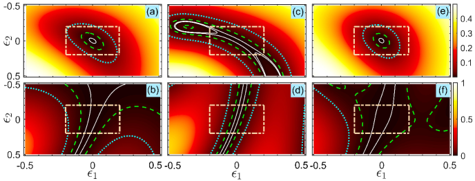
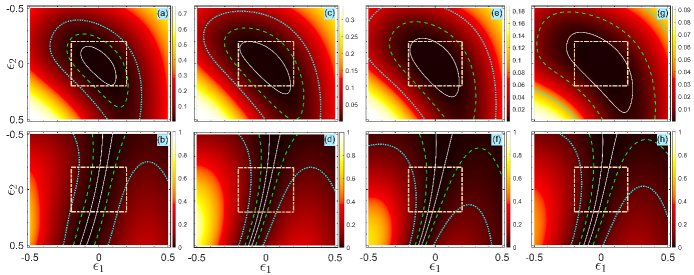
Figure 2 demonstrates the infidelity and the population leakage as a function of the deviations and by different cost functions. Compared Figs. 2(a)-2(b) with Fig. 1, both the robust behaviors and the population leakage are slightly improved when we choose the cost function . An inspection of Figs. 2(c)-2(d) demonstrates that population transfer would be more accurate when the phases are determined by Eq. (17), since the region enclosed by white-solid curves in Fig. 2(c) is much larger than that in Fig. 2(a). Nevertheless, there are plenty of population leakages in this situation. When adopting the phases determined by Eq. (18), the population leakage is suppressed at a very low level in a wide region, as shown in Fig. 2(f). These results show that the robust behaviors are quite different when we choose different cost functions.
III.2 Three pulses
The form of the three-pulse sequence is expressed by
and the zeroth-order coefficient in Eq. (9) becomes
| (20) |
where and , . The first-order coefficients and in Eq. (9) are
| (22) | |||||
For the second-order coefficients, since the expressions are too complicated to present here, we give them in Appendix C.
It is easily found that one solution of equations reads
where when , while when . Note that there are four variables (, , , and ) in the three-pulse sequence, and the values of the variables and are given by Eq. (III.2). Therefore, only two variables and can be designed to eliminate the influence of the deviations. In the following, the cost function is chosen as , that is, the impact of the accuracy of population transfer and the leakage to the excited state are equally weighted in the three-pulse sequence.
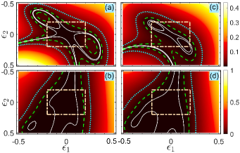
Figure 3 shows the performance of the infidelity and the population leakage in the three-pulse sequence. It can be seen that both the infidelity and the population leakage keep a very small value in the presence of strong deviations. Compared with the case of the resonant pulses (cf. Fig. 1), the region becomes much wider in the three-pulse sequence, and thus this sequence is more robust against the deviations and . Noting that it is hard to obtain the analytical expressions for the phases and in the three-pulse sequence, we present some numerical solutions for different populations (i.e., different ) in Table 1.
| 3-pulse sequence | 4-pulse sequence | 5-pulse sequence | |
| /2 | 3.911 3.142 2.340 3.142 | 3.195 4.817 1.831 1.630 0.110 4.983 | 5.291 2.472 1.925 6.089 1.325 5.943 4.238 6.095 |
| /3 | 2.663 5.027 1.562 0.189 | 2.769 5.550 1.526 5.762 5.401 2.275 | 2.707 5.876 2.868 5.175 6.032 2.260 1.730 5.963 |
| /4 | 2.497 4.859 1.450 0.670 | 3.554 2.374 6.030 2.768 4.729 6.027 | 3.575 1.214 2.962 6.015 4.985 4.848 2.674 4.759 |
| /5 | 3.828 1.466 4.894 5.313 | 3.514 1.885 5.420 2.786 4.299 5.850 | 3.285 0.744 4.382 1.603 4.232 4.050 5.108 3.656 |
| /6 | 3.870 1.508 4.971 5.155 | 3.514 1.047 4.429 2.852 3.527 5.200 | 3.317 0.802 4.516 1.688 4.266 4.106 5.013 3.469 |
| /7 | 3.911 1.550 5.048 5.070 | 5.431 3.456 3.162 4.786 5.953 4.117 | 2.677 4.582 0.254 3.172 3.787 3.449 3.913 5.049 |
| /10 | 3.953 1.550 5.179 4.883 | 3.408 0.733 4.039 2.840 3.307 5.417 | 5.948 2.591 4.891 3.048 3.871 5.556 5.753 5.134 |
| /20 | 1.664 3.267 3.038 0.174 | 6.283 3.351 3.665 5.853 6.063 5.633 | 1.837 0.585 4.787 4.277 3.287 0.220 3.388 0.247 |
III.3 More than three pulses
The form of the four-pulse sequence reads
and the zeroth-order coefficient in Eq. (9) becomes
| (24) | |||||
where and , . The first-order coefficients and in Eq. (9) are expressed by
| (25) | |||||
Thus, one solution of equations can be written as
As a result, there are still four variables available to eliminate the influence of the deviations in the four-pulse sequence, and some numerical solutions for different are presented in Table 1.
Similarly, the zeroth-order in the five-pulse sequence can be expressed by
| (26) | |||||
Due to the complex expressions of the first-order coefficients, we present it in Appendix D. After satisfying , there are still six variables to eliminate the influence of the deviations in the five-pulse sequence, and some numerical solutions for different are presented in Table 1.
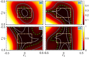
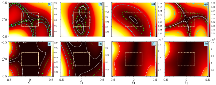
Figure 4 shows the infidelity and the population leakage as a function of the deviations in the four(five)-pulse sequence. One can find from Fig. 4 that the infidelity and the population leakage are small in a wider region as the number of pulses increase. Apparently, the population transfer would be more accurate when more pulses are taken into account. Note that the cost function is chosen as in Fig. 4, namely, the impact of the accuracy of the population transfer and the leakage to the excited state are equally weighted. We present in Appendix E the detailed discussion on the performance of the accuracy and the leakage by choosing different forms of cost functions.
Next, we demonstrate the evolutionary trajectory of the qubit (i.e., the ground states and ) on the Bloch sphere under the -pulse sequence. Taking the four-pulse sequence as an example, suppose the initial state of this system is . Then, the final state of this system after the four-pulse sequence can be expressed in the basis by employing four angle variables:
| (30) |
Since we focus on the evolutionary trajectory of the qubit, the phase is irrelevant and we can simply write the time evolution of qubit as: . When , the evolutionary trajectory is on the Bloch sphere. While it is inside the Bloch sphere when . Here, the state inside the Bloch sphere does not represent the mixed state, and means the population leakage from ground states to the excited state. Note that the smaller the value of is, the larger the population leakage will be. The center of the Bloch sphere, i.e., , represents the excited state .
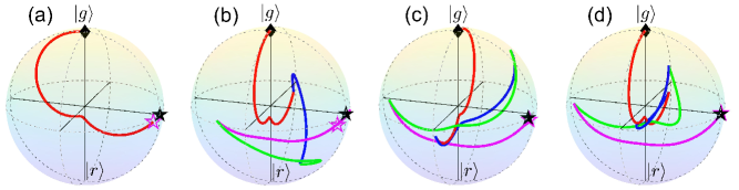
Figures 5(b)-5(d) show the evolutionary trajectories of the qubit for different cost functions in the four-pulse sequence. By contrast, we plot in Fig. 5(a) the evolutionary trajectory for the resonant pulses. We can observe from Fig. 5 that the population leakage always exists during the evolution process, since the trajectories are inside the Bloch sphere in some evolution stages. Nevertheless, the population leakage is strongly suppressed and the system state approaches the target state at the final time, as shown in Fig. 5(d). It is shown in Fig. 5(b) that the cost function only guarantees the accuracy of , while there exists leakage to the excited state. As a result, the final state deviates from the target state. A similar situation is also found in Fig. 5(c), because the cost function only prevents the population leakage to the excited state. However, Fig. 5(d) demonstrates that the system is almost driven into the target state, because the cost function is a tradeoff between the accuracy and the population leakage. Note that the corresponding robust region designed by (e.g., the region enclosed by the white-curves in Fig. 4) is generally smaller than those designed by the other two cost functions. For details, one can see Appendix E.
IV Applications: Robust preparation of three-atom singlet state by composite pulses
In above section, we have showed the design process of composite pulses in a general physical system, where the three-level structure can be found in atomic systems Scully and Zubairy (1997), trapped ions Leibfried et al. (2003), diamond nitrogen-vacancy centers Yang et al. (2010), and superconducting circuits Xiang et al. (2013); Xue et al. (2017); Kang et al. (2016, 2017); Hong et al. (2018); Chen et al. (2020), etc. In this section, we demonstrate that the CPs scheme can be also generalized to complicated systems for performing different quantum tasks, e.g., coherent conversion between two qubits Yang et al. (2021) or preparation of entangled states Shao et al. (2010), etc. The fundamental is to reduce complicated systems to the familiar three-level physical model. As an example, in presence of deviations, we next prepare the three-atom singlet state with ultrahigh fidelity in an atom-cavity system, and this approach is easily extended to other complicated systems.
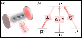
As shown in Fig. 6(a), consider the atom-cavity system, where three identical four-level atoms are trapped in a bimodal cavity. The four-level atom has three ground states , , and , and an excited state , as shown in Fig. 6(b). The transition () is resonantly coupled by the cavity mode () with the coupling constant (), where the subscript represents the th atom. The transition is resonantly coupled by the laser field with the coupling strength and the phase . In the interaction picture, the Hamiltonian of the atom-cavity system reads ()
| (31) | |||||
where and are the annihilation operators of the cavity mode and , respectively. and () are respectively the deviations of the laser fields and the cavity mode due to the inhomogeneities of spatial distribution.
Apparently, the excited number is a conserved quantity in this system since , where the excited number operator is defined by . When the condition () is satisfied, we can restrict the system dynamics into the single-excited subspace and the Hamiltonian is approximated by Shao et al. (2010)
| (32) | |||||
where we set , , , and
The state represents the first atom in , the second atom in , and the third atom in . Since the cavity mode () is in vacuum state, we have ignored it in the Hamiltonian given by Eq. (32).
It is easily found from Eq. (32) that the atom-cavity system can be reduced to the three-level physical model studied in Sec. II. Hence, if the initial state of this system is , by fixing the ratio of two coupling coefficients and modulating the phases according to the above composite pulses theory, one can obtain the following superposition state
| (33) |
By setting and , the state becomes
which is actually the three-atom singlet state.
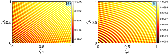
We first explore how the deviations of two coupling constants and affect the fidelity of the singlet state. The numerical results simulated by the three-pulse sequence scheme are shown in Fig. 7(a), where we choose to guarantee the validity of the effective Hamiltonian given by Eq. (32) (i.e., the condition is well satisfied). As a comparison, we also plot in Fig. 7(b) the fidelity as a function of the deviations and by the resonant pulses scheme shown in Ref. Shao et al. (2010). The results demonstrate that both schemes are robust against the deviations in two coupling constants, since the impact on the fidelity can be negligible no matter how large the deviations are, cf., in Fig. 7. The reason for this phenomenon is that both and are absent in the Hamiltonian given by Eq. (32). Besides, an interesting finding is that the fidelity tends to a higher value when the deviations and are much larger. A reasonable interpretation is given as follows. During the process of deriving the Hamiltonian given by Eq. (32), the strong coupling condition () is exploited. The coupling constant () increases with the raising of the deviation . As a result, the dynamics of this system is more and more restricted in the single-excited subspace so that the Hamiltonian given by Eq. (32) ensures a better validity for suppressing the leakage to other subspaces. Thus, a higher fidelity of the singlet state can be achieved when a larger deviation appears.
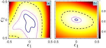
Next, we address the influence of the two deviations and on the fidelity . In Fig. 8(a), we display the fidelity versus the deviations and for the three-pulse sequence. For comparison, we also plot in Fig. 8(b) the performance of the fidelity for the resonant pulses scheme shown in Ref. Shao et al. (2010). As shown by the area surrounded by the blue-solid (or pink-dotted) curve in Fig. 8(b), it is clear that the scheme shown in Ref. Shao et al. (2010) is highly susceptible to the deviations and . However, the fidelity of the singlet state obtained by the three-pulse sequence remains in a high value () even when a very large deviation occurs. This benefits from the fact that the second-order coefficients of systematic errors are restricted to an extremely low value by the specific set of phases. Furthermore, as the pulse number increases, the higher-order coefficients can be restricted to a low value that ensures a robust behavior against the deviations and . Thus, the CPs sequence can further improve an error-tolerant performance of the singlet state.
Another experimental issue, which inevitably impacts the performance of the final fidelity, is the waveform distortion. In the ideal condition, our input pulse shape is associated with a perfect square waveform. However, in practice, the input square wave always produces a tiny smooth rising and falling edge. Let us study this issue by taking the three-pulse sequence as an example. First of all, we design a group of functions in which the waveform distortion can be arbitrarily adjustable. The functions are given by
| (34) |
| (35) |
where . Here, is a dimensionless parameter that defines the magnitude of the rising and falling edge of the square wave.
As increases, the functions (34) and (35) gradually become a square wave. Specifically from Fig. 9(a) and 9(b), we see that the functions are almost square waveforms for =1000 (the blue-dotted curves). For , they describe perfect square waves. However, when is small, e.g., =10, the duration of the rising and falling edge of the square wave becomes excessively long and the waveform has a serious shape change. Then, functions (34) and (35) turn into a smooth time-dependent pulse, as shown by the red-dashed curves in Fig. 9(a) and 9(b). Obviously, this kind of waveform does not satisfy the request of our CPs scheme. As illustrated in Fig. 9(c), even though the waveform suffers from serious distortion (the red-dashed curve), the fidelity can still maintain a high value ( 0.99). Moreover, as revealed by the cyan-solid and pink-dashed-dotted curves in Fig. 9(c), a slight distortion in the waveform hardly makes an impact on the final fidelity. Hence, the CPs sequence has the ability to acquire a precise and robust singlet state even with a distorted waveform. Finally, we investigate the influence of the phase shift errors on the fidelity. In presence of the deviations in the phases, the actual phases can be rewritten as
| (36) |
where and represent the phase shift errors. We plot in Fig. 9(d) the relation between the fidelity and the phase shift errors, which shows that the current CPs sequence is sensitive to phase shift errors Torosov et al. (2021). The reason is that we do not consider the phase shift errors in the Hamiltonian given by Eq. (3). To tackle this problem, one requires to regard the phase shift errors as variables in Eq. (3), and then constructs a phase-error-corrected composite pulses sequence Torosov and Vitanov (2019c).
In a more realistic situation, one has to consider the influence of decoherence on the fidelity of the singlet state. In this system, the decoherence mainly comes from two aspects: () the atomic spontaneous emission from the excited state to the ground states. () the decay of two cavity modes. Under the decoherence environment, the dynamics of this system are governed by the Lindblad master equation and the form can be written as
| (37) |
where and the Lindblad super-operator is
| (38) |
where is the standard Lindblad operator. and () are the dissipation rate from the excited state to the ground state and the decay rate of the cavity mode (), respectively. For simplicity, we set and .
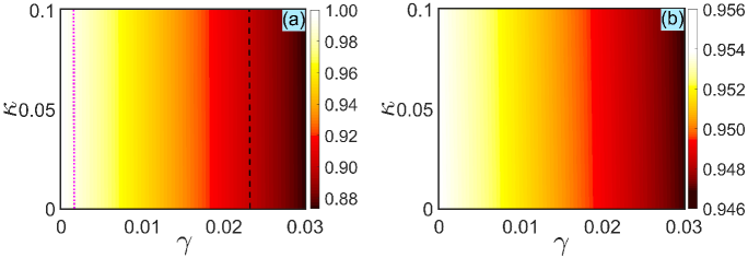
Figure 10 displays the fidelity as a function of the dissipation rate and the decay rate by both the three-pulse sequence scheme and the resonant pulses scheme shown in Ref. Shao et al. (2010). We observe from Fig. 10(b) that the fidelity cannot maintain a relatively high value in the resonant pulses scheme even if the system does not suffer from the decoherence, cf., in Fig. 10(b). However, in the three-pulse sequence scheme, the fidelity can reach a high value () when the dissipation rate is small, cf., the left region of the pink-dotted line in Fig. 10(a). Another intriguing aspect in Fig. 10 is that the fidelity does not sharply drop in the resonant pulses scheme while the range of fidelity varies widely in the three-pulse sequence scheme. This is because the evolution time in the resonant pulses scheme is much shorter than that in the three-pulse sequence scheme. As a result, the influence of the decoherence on the system is relatively small by the resonant pulses scheme. From this point, we find that the longer pulse sequence is not the optimal choice in a severe decoherence environment, even though the longer pulse sequence can help to improve the robustness of the system. Furthermore, according to the pink-dotted line in Fig. 10(a), it is seen that the influence of the cavity decay is almost negligible, since even when the decay rate increases to 0.1. This phenomenon can be explained by the fact that the strong coupling constant ensures the decoupling of the single-photon state to minimize the loss of the cavity decay. From a physical point of view, the cavity is regarded as intermediary to realize indirect coupling between atoms, and it is almost in the vacuum state under the strong coupling condition.
On the other hand, for a given cavity decay rate, the fidelity decreases with the increase of the dissipation rate . Thus, the major influence on the preparation of single state is atomic spontaneous emission. The physical mechanism can be clarified as follows. Under the strong coupling condition (), the dynamics of the system can be approximately described by the Hamiltonian in Eq. (32). To obtain the singlet state, we need to utilize the intermediate state . Nevertheless, we can see that contains the excited states (), which cannot be effectively eliminated during the evolution process. Hence, the dynamics of the system is sensitive to the spontaneous emission. An alternative approach to solve this problem is to adiabatically eliminate the excited state Brion et al. (2007); Vitanov et al. (2017), i.e., adopting the Raman transition process. To be specific, the one-photon detuning between the excited state and the ground states is large enough, while the system satisfies the two-photon resonance condition. Then, the population of the intermediate state is sharply suppressed, and the population can adiabatically transfer between ground states during the evolution. As a result, the influence of the spontaneous emission is effectively eliminated.
V Conclusion
In this work, we achieved a high fidelity population transfer for the three-level system by the CPs sequence. We derived the transition probability from the total propagator and used the Taylor expansion to disassemble it into a series of derivatives. For a small number of pulses, since not enough variables (phases) can be employed to eliminate anticipated deviations, we constructed a cost function to control the fidelity of the result. Then, we showed that high fidelity of the target state, or suppressing the population of the leakage state, or both two objectives are robustly achievable by choosing different forms of cost functions. Particularly, the method of the short pulse sequence can be further extended to a longer one if necessary.
As an example, we applied the CPs sequence to implement the three-atom singlet state with ultrahigh fidelity in the atom-cavity system, where we only needed to individually control the phase of the inputting pulses. The numerical results indicate that the final singlet state is robust against the deviations in two coupling coefficients. Moreover, we found that significant distortion in the pulse sequence has a very small impact on the fidelity of the singlet state. As the simulated results further reveal, the fidelity of the final singlet state keeps a relatively high value in the decoherence environment. Our CPs scheme provides a selectable way for robust controlling in the error-prone environment and shows an enormous potential application in various physical models, e.g., implementation of coherently convertible dual-type qubits with high fidelity Yang et al. (2021).
Acknowledgements.
This work is supported by the National Natural Science Foundation of China under Grant Nos. 11874114, 12175033, 12147206, 11805036, the Natural Science Foundation of Fujian Province under Grant No. 2021J01575, the Natural Science Funds for Distinguished Young Scholar of Fujian Province under Grant 2020J06011, and the Project from Fuzhou University under Grant JG202001-2.Appendix A The detailed derivation of the total propagator without deviations in the composite -pulse sequence
In this appendix, we first calculate the general expression of the propagator for each pulse, and then give out the total propagator of the composite -pulse sequence.
In absence of the deviations, the Hamiltonian of the th pulse can be written as ()
By choosing the pulse duration , the matrix form of the corresponding propagator in the basis becomes (up to a global phase)
| (45) |
where
Since the ground states are decoupled from the excited state and the qubit subspace is of interest, we can only employ matrix of the propagator in the following.
Next, we calculate the propagator of the first two pulses, which reads
| (52) |
where
One can easily find that the propagator has the same form as that of the single pulse. Therefore, we can assume that the propagator of the first pulses has the following form ()
| (55) |
Then, the propagator of the first pulses becomes
| (60) | |||||
| (63) |
From Eq. (60), we have the following recursive relations:
| (64) |
Therefore, the total propagator of the composite -pulse sequence becomes
| (67) |
where , , and satisfy the recursive relations given by Eq. (A). The population of the ground state reads
| (68) |
Appendix B The second-order coefficients in the two-pulse sequence
In this appendix, we give the expressions of the second-order coefficients and (), in terms of , which read
With these coefficients, we can evaluate the cost functions. First, the expression of the cost function is
As a result, it is not hard to calculate that the cost function is minimal when
where . Second, the expression of the cost function is
Obviously, is minimal when
Finally, the cost function is minimal when
Here, is the solution of the following quartic equation:
where the coefficients () are:
Appendix C The second-order coefficients in the three-pulse sequence
In this appendix, we give the expressions of the second-order coefficients and () in the three-pulse sequence, which read
| (74) | |||||
| (82) | |||||
| (90) | |||||
| (94) | |||||
| (98) | |||||
where and ().
Appendix D The first-order coefficients in the five-pulse sequence
In this appendix, we provide the expressions of the first-order coefficients in the five-pulse sequence, which are
where and ().
Appendix E Detailed discussion on the performance of the accuracy and leakage in the four-pulse sequence
In this appendix, taking the four-pulse sequence as an example, we discuss in detail the influence of different cost functions on the performance of the accuracy and the leakage. As stated in Sec. II, the cost functions are mainly divided into three types: () is meant to eliminate the deviations in ; () is aimed to eliminate the population leakage ; () is a combination of both, intended to eliminate both the deviations in and the population leakage .
Figure 11, Figure 12, and Figure 13 are the plotted infidelity and population leakage as a function of deviations through the cost functions , , and , respectively. The results demonstrate that in Fig. 11 is much more accurate than those in Figs. 12 and Fig. 13, while the population leakage in Fig. 12 is much smaller than those in Figs. 11 and Fig. 13. In Fig. 13, there is a tradeoff between the accuracy and the leakage. Therefore, different cost functions have different effects, and one can choose a specific cost function according to the particular task in quantum information processing.
| Fig. 5(b) | /4 | 0.0003 | 6.0928 | 4.6077 | 1.2835 | 2.1652 | 3.8217 | 1.2823 |
| Fig. 5(c) | /4 | 0.0004 | 3.6176 | 0.5585 | 3.1750 | 4.3222 | 4.4047 | 6.1550 |
| Fig. 5(d) | /4 | 0.0007 | 3.5541 | 2.3736 | 6.0291 | 2.7675 | 4.7286 | 6.0267 |
| Figs. 11(a)-11(b) | /3 | 0.0054 | 3.0883 | 5.0265 | 1.7134 | 2.1955 | 0.9921 | 0.9750 |
| Figs. 11(c)-11(d) | /5 | 0.0015 | 3.3013 | 0.0000 | 2.9063 | 2.5848 | 2.4251 | 3.3583 |
| Figs. 11(e)-11(f) | /7 | 0.0014 | 3.1948 | 5.1313 | 2.0471 | 4.7325 | 3.5274 | 1.0833 |
| Figs. 11(g)-11(h) | /10 | 0.0010 | 3.3013 | 0.6283 | 3.6638 | 4.4918 | 4.9604 | 2.2749 |
| Figs. 12(a)-12(b) | /3 | 0.0021 | 3.9403 | 0.9425 | 3.0538 | 4.7064 | 4.8502 | 5.6332 |
| Figs. 12(c)-12(d) | /5 | 0.0009 | 3.5143 | 3.6652 | 1.2319 | 2.6600 | 5.9525 | 1.4083 |
| Figs. 12(e)-12(f) | /7 | 0.0010 | 3.1948 | 0.1047 | 3.1443 | 3.6964 | 3.7479 | 0.1083 |
| Figs. 12(g)-12(h) | /10 | 3.4078 | 0.2094 | 3.0884 | 3.6944 | 3.6376 | 6.1749 | |
| Figs. 13(a)-13(b) | /3 | 0.0027 | 2.7689 | 5.5501 | 1.5253 | 5.7617 | 5.4013 | 2.2749 |
| Figs. 13(c)-13(d) | /5 | 0.0025 | 3.5143 | 1.8850 | 5.4201 | 2.7867 | 4.2990 | 5.8499 |
| Figs. 13(e)-13(f) | /7 | 0.0036 | 3.4603 | 1.9897 | 5.4838 | 2.8304 | 4.5014 | 0.1848 |
| Figs. 13(g)-13(h) | /10 | 0.0014 | 3.4078 | 0.7330 | 4.0386 | 2.8401 | 3.3069 | 5.4165 |
References
- Salières et al. (1995) P. Salières, A. L’Huillier, and M. Lewenstein, Coherence Control of High-Order Harmonics, Phys. Rev. Lett. 74, 3776 (1995).
- Bergmann et al. (1998) K. Bergmann, H. Theuer, and B. W. Shore, Coherent population transfer among quantum states of atoms and molecules, Rev. Mod. Phys. 70, 1003 (1998).
- Makhlin et al. (2001) Y. Makhlin, G. Schön, and A. Shnirman, Quantum-state engineering with Josephson-junction devices, Rev. Mod. Phys. 73, 357 (2001).
- Zhao et al. (2006) H. Zhao, E. J. Loren, H. M. van Driel, and A. L. Smirl, Coherence Control of Hall Charge and Spin Currents, Phys. Rev. Lett. 96, 246601 (2006).
- McCullough et al. (2000) E. McCullough, M. Shapiro, and P. Brumer, Coherent control of refractive indices, Phys. Rev. A 61, 041801 (2000).
- Gordon et al. (2002) R. Gordon, A. P. Heberle, A. J. Ramsay, and J. R. A. Cleaver, Experimental coherent control of lasers, Phys. Rev. A 65, 051803 (2002).
- Zeng et al. (2020) Z.-Y. Zeng, L. Li, B. Yang, J. Xiao, and X. Luo, Coherent control of dissipative dynamics in a periodically driven lattice array, Phys. Rev. A 102, 012221 (2020).
- Devolder et al. (2021) A. Devolder, P. Brumer, and T. V. Tscherbul, Complete Quantum Coherent Control of Ultracold Molecular Collisions, Phys. Rev. Lett. 126, 153403 (2021).
- Levine et al. (2018) H. Levine, A. Keesling, A. Omran, H. Bernien, S. Schwartz, A. S. Zibrov, M. Endres, M. Greiner, V. Vuletić, and M. D. Lukin, High-Fidelity Control and Entanglement of Rydberg-Atom Qubits, Phys. Rev. Lett. 121, 123603 (2018).
- Daems et al. (2013) D. Daems, A. Ruschhaupt, D. Sugny, and S. Guérin, Robust Quantum Control by a Single-Shot Shaped Pulse, Phys. Rev. Lett. 111, 050404 (2013).
- Allen and Eberly (1975) L. Allen and J. H. Eberly, Optical resonance and two-level atoms (New York: Dover Publications, 1975).
- Vitanov et al. (2001) N. V. Vitanov, T. Halfmann, B. W. Shore, and K. Bergmann, Laser-induced population transfer by adiabatic passage techniques, Annu. Rev. Phys. Chem. 52, 763 (2001).
- Guéry-Odelin et al. (2019) D. Guéry-Odelin, A. Ruschhaupt, A. Kiely, E. Torrontegui, S. Martínez-Garaot, and J. G. Muga, Shortcuts to adiabaticity: Concepts, methods, and applications, Rev. Mod. Phys. 91, 045001 (2019).
- Scully and Zubairy (1997) M. O. Scully and M. S. Zubairy, Quantum Optics (Cambridge University Press, 1997).
- Gerry and Knight (2004) C. Gerry and P. Knight, Introductory Quantum Optics (Cambridge University Press, 2004).
- Shankar (1994) R. Shankar, Principles of Quantum Mechanics (Springer US, 1994).
- Král et al. (2007) P. Král, I. Thanopulos, and M. Shapiro, Colloquium: Coherently controlled adiabatic passage, Rev. Mod. Phys. 79, 53 (2007).
- Wimperis (1991) S. Wimperis, Iterative schemes for phase-distortionless composite 180° pulses, J. Magn. Reson. 93, 199 (1991).
- Wimperis (1994) S. Wimperis, Broadband, Narrowband, and Passband Composite Pulses for Use in Advanced NMR Experiments, J. Magn. Reson. 109, 221 (1994).
- Levitt and Freeman (1979) M. H. Levitt and R. Freeman, NMR population inversion using a composite pulse, J. Magn. Reson. 33, 473 (1979).
- Levitt (1986) M. H. Levitt, Composite pulses, Prog. NMR Spectrosc. 18, 61 (1986).
- Brown et al. (2004) K. R. Brown, A. W. Harrow, and I. L. Chuang, Arbitrarily accurate composite pulse sequences, Phys. Rev. A 70, 052318 (2004).
- Dridi et al. (2020) G. Dridi, M. Mejatty, S. J. Glaser, and D. Sugny, Robust control of a NOT gate by composite pulses, Phys. Rev. A 101, 012321 (2020).
- Torosov and Vitanov (2011) B. T. Torosov and N. V. Vitanov, Smooth composite pulses for high-fidelity quantum information processing, Phys. Rev. A 83, 053420 (2011).
- Genov et al. (2014) G. T. Genov, D. Schraft, T. Halfmann, and N. V. Vitanov, Correction of Arbitrary Field Errors in Population Inversion of Quantum Systems by Universal Composite Pulses, Phys. Rev. Lett. 113, 043001 (2014).
- Torosov and Vitanov (2018) B. T. Torosov and N. V. Vitanov, Arbitrarily accurate twin composite -pulse sequences, Phys. Rev. A 97, 043408 (2018).
- Jones (2013) J. A. Jones, Designing short robust not gates for quantum computation, Phys. Rev. A 87, 052317 (2013).
- Vitanov (2011) N. V. Vitanov, Arbitrarily accurate narrowband composite pulse sequences, Phys. Rev. A 84, 065404 (2011).
- Torosov and Vitanov (2019a) B. T. Torosov and N. V. Vitanov, Robust high-fidelity coherent control of two-state systems by detuning pulses, Phys. Rev. A 99, 013424 (2019a).
- Torosov et al. (2020a) B. T. Torosov, S. S. Ivanov, and N. V. Vitanov, Narrowband and passband composite pulses for variable rotations, Phys. Rev. A 102, 013105 (2020a).
- Genov et al. (2020) G. T. Genov, M. Hain, N. V. Vitanov, and T. Halfmann, Universal composite pulses for efficient population inversion with an arbitrary excitation profile, Phys. Rev. A 101, 013827 (2020).
- Torosov et al. (2015) B. T. Torosov, E. S. Kyoseva, and N. V. Vitanov, Composite pulses for ultrabroad-band and ultranarrow-band excitation, Phys. Rev. A 92, 033406 (2015).
- Ichikawa et al. (2011) T. Ichikawa, M. Bando, Y. Kondo, and M. Nakahara, Designing robust unitary gates: Application to concatenated composite pulses, Phys. Rev. A 84, 062311 (2011).
- Cohen et al. (2016) I. Cohen, A. Rotem, and A. Retzker, Refocusing two-qubit-gate noise for trapped ions by composite pulses, Phys. Rev. A 93, 032340 (2016).
- Kyoseva et al. (2019) E. Kyoseva, H. Greener, and H. Suchowski, Detuning-modulated composite pulses for high-fidelity robust quantum control, Phys. Rev. A 100, 032333 (2019).
- Wang et al. (2014) X. Wang, L. S. Bishop, E. Barnes, J. P. Kestner, and S. D. Sarma, Robust quantum gates for singlet-triplet spin qubits using composite pulses, Phys. Rev. A 89, 022310 (2014).
- Mount et al. (2015) E. Mount, C. Kabytayev, S. Crain, R. Harper, S.-Y. Baek, G. Vrijsen, S. T. Flammia, K. R. Brown, P. Maunz, and J. Kim, Error compensation of single-qubit gates in a surface-electrode ion trap using composite pulses, Phys. Rev. A 92, 060301 (2015).
- Demeter (2016) G. Demeter, Composite pulses for high-fidelity population inversion in optically dense, inhomogeneously broadened atomic ensembles, Phys. Rev. A 93, 023830 (2016).
- Ivanov and Vitanov (2011) S. S. Ivanov and N. V. Vitanov, High-fidelity local addressing of trapped ions and atoms by composite sequences of laser pulses, Opt. Lett. 36, 1275 (2011).
- Torosov and Vitanov (2019b) B. T. Torosov and N. V. Vitanov, Arbitrarily accurate variable rotations on the Bloch sphere by composite pulse sequences, Phys. Rev. A 99, 013402 (2019b).
- Vandersypen and Chuang (2005) L. M. K. Vandersypen and I. L. Chuang, NMR techniques for quantum control and computation, Rev. Mod. Phys. 76, 1037 (2005).
- Fleischhauer et al. (2005) M. Fleischhauer, A. Imamoglu, and J. P. Marangos, Electromagnetically induced transparency: Optics in coherent media, Rev. Mod. Phys. 77, 633 (2005).
- Scully et al. (1989) M. O. Scully, S.-Y. Zhu, and A. Gavrielides, Degenerate quantum-beat laser: Lasing without inversion and inversion without lasing, Phys. Rev. Lett. 62, 2813 (1989).
- Levitt et al. (1984) M. H. Levitt, D. Suter, and R. R. Ernst, Composite pulse excitation in three-level systems, J. Chem. Phys. 80, 3064 (1984).
- Ramamoorthy and Narasimhan (1991) A. Ramamoorthy and P. Narasimhan, Phase-alternated composite /2 pulses for solid state quadrupole echo NMR spectroscopy, Pramana 36, 399 (1991).
- Torosov et al. (2011) B. T. Torosov, S. Guérin, and N. V. Vitanov, High-Fidelity Adiabatic Passage by Composite Sequences of Chirped Pulses, Phys. Rev. Lett. 106, 233001 (2011).
- Torosov and Vitanov (2013) B. T. Torosov and N. V. Vitanov, Composite stimulated Raman adiabatic passage, Phys. Rev. A 87, 043418 (2013).
- Schraft et al. (2013) D. Schraft, T. Halfmann, G. T. Genov, and N. V. Vitanov, Experimental demonstration of composite adiabatic passage, Phys. Rev. A 88, 063406 (2013).
- Ishida et al. (2018) N. Ishida, T. Nakamura, T. Tanaka, S. Mishima, H. Kano, R. Kuroiwa, Y. Sekiguchi, and H. Kosaka, Universal holonomic single quantum gates over a geometric spin with phase-modulated polarized light, Opt. Lett. 43, 2380 (2018).
- Torosov et al. (2020b) B. T. Torosov, M. Drewsen, and N. V. Vitanov, Chiral resolution by composite Raman pulses, Phys. Rev. Research 2, 043235 (2020b).
- Lehmann (2018) K. K. Lehmann, Influence of spatial degeneracy on rotational spectroscopy: Three-wave mixing and enantiomeric state separation of chiral molecules, J. Chem. Phys. 149, 094201 (2018).
- Leibscher et al. (2019) M. Leibscher, T. F. Giesen, and C. P. Koch, Principles of enantio-selective excitation in three-wave mixing spectroscopy of chiral molecules, J. Chem. Phys. 151, 014302 (2019).
- Genov et al. (2011) G. T. Genov, B. T. Torosov, and N. V. Vitanov, Optimized control of multistate quantum systems by composite pulse sequences, Phys. Rev. A 84, 063413 (2011).
- Torosov and Vitanov (2020) B. T. Torosov and N. V. Vitanov, High-fidelity composite quantum gates for Raman qubits, Phys. Rev. Research 2, 043194 (2020).
- Morris and Shore (1983) J. R. Morris and B. W. Shore, Reduction of degenerate two-level excitation to independent two-state systems, Phys. Rev. A 27, 906 (1983).
- Majorana (1932) E. Majorana, Atomi orientati in campo magnetico variabile, Nuovo Cimento 9, 43 (1932).
- Ghosh et al. (2017) J. Ghosh, S. N. Coppersmith, and M. Friesen, Pulse sequences for suppressing leakage in single-qubit gate operations, Phys. Rev. B 95, 241307 (2017).
- Shi et al. (2021) Z.-C. Shi, H.-N. Wu, L.-T. Shen, J. Song, Y. Xia, X. X. Yi, and S.-B. Zheng, Robust single-qubit gates by composite pulses in three-level systems, Phys. Rev. A 103, 052612 (2021).
- Leibfried et al. (2003) D. Leibfried, R. Blatt, C. Monroe, and D. Wineland, Quantum dynamics of single trapped ions, Rev. Mod. Phys. 75, 281 (2003).
- Yang et al. (2010) W. Yang, Z. Xu, M. Feng, and J. Du, Entanglement of separate nitrogen-vacancy centers coupled to a whispering-gallery mode cavity, New J. Phys. 12, 113039 (2010).
- Xiang et al. (2013) Z.-L. Xiang, S. Ashhab, J. Q. You, and F. Nori, Hybrid quantum circuits: Superconducting circuits interacting with other quantum systems, Rev. Mod. Phys. 85, 623 (2013).
- Xue et al. (2017) Z.-Y. Xue, F.-L. Gu, Z.-P. Hong, Z.-H. Yang, D.-W. Zhang, Y. Hu, and J. Q. You, Nonadiabatic Holonomic Quantum Computation with Dressed-State Qubits, Phys. Rev. Applied 7, 054022 (2017).
- Kang et al. (2016) Y.-H. Kang, Y.-H. Chen, Z.-C. Shi, J. Song, and Y. Xia, Fast preparation of states with superconducting quantum interference devices by using dressed states, Phys. Rev. A 94, 052311 (2016).
- Kang et al. (2017) Y.-H. Kang, Y.-H. Chen, Z.-C. Shi, B.-H. Huang, J. Song, and Y. Xia, Complete Bell-state analysis for superconducting-quantum-interference-device qubits with a transitionless tracking algorithm, Phys. Rev. A 96, 022304 (2017).
- Hong et al. (2018) Z.-P. Hong, B.-J. Liu, J.-Q. Cai, X.-D. Zhang, Y. Hu, Z. D. Wang, and Z.-Y. Xue, Implementing universal nonadiabatic holonomic quantum gates with transmons, Phys. Rev. A 97, 022332 (2018).
- Chen et al. (2020) T. Chen, P. Shen, and Z.-Y. Xue, Robust and Fast Holonomic Quantum Gates with Encoding on Superconducting Circuits, Phys. Rev. Applied 14, 034038 (2020).
- Greentree et al. (2004) A. D. Greentree, J. H. Cole, A. R. Hamilton, and L. C. L. Hollenberg, Coherent electronic transfer in quantum dot systems using adiabatic passage, Phys. Rev. B 70, 235317 (2004).
- Bruderer et al. (2012) M. Bruderer, K. Franke, S. Ragg, W. Belzig, and D. Obreschkow, Exploiting boundary states of imperfect spin chains for high-fidelity state transfer, Phys. Rev. A 85, 022312 (2012).
- Chen and Li (2016) B. Chen and Y. Li, Coherent state transfer through a multi-channel quantum network: Natural versus controlled evolution passage, Sci. China Phys. Mech. Astron. 59, 640302 (2016).
- Li and Shao (2018) D. X. Li and X. Q. Shao, Unconventional Rydberg pumping and applications in quantum information processing, Phys. Rev. A 98, 062338 (2018).
- Kang et al. (2018) Y.-H. Kang, Y.-H. Chen, Z.-C. Shi, B.-H. Huang, J. Song, and Y. Xia, Nonadiabatic holonomic quantum computation using Rydberg blockade, Phys. Rev. A 97, 042336 (2018).
- Shi et al. (2018) Z.-C. Shi, D. Ran, L.-T. Shen, Y. Xia, and X. X. Yi, Quantum state engineering by periodical two-step modulation in an atomic system, Opt. Express 26, 34789 (2018).
- Li et al. (2020) R. Li, D. Yu, S.-L. Su, and J. Qian, Periodically driven facilitated high-efficiency dissipative entanglement with Rydberg atoms, Phys. Rev. A 101, 042328 (2020).
- Shao (2020) X.-Q. Shao, Selective Rydberg pumping via strong dipole blockade, Phys. Rev. A 102, 053118 (2020).
- Wu et al. (2021) J.-L. Wu, Y. Wang, J.-X. Han, S.-L. Su, Y. Xia, Y. Jiang, and J. Song, Resilient quantum gates on periodically driven Rydberg atoms, Phys. Rev. A 103, 012601 (2021).
- Taie et al. (2020) S. Taie, T. Ichinose, H. Ozawa, and Y. Takahashi, Spatial adiabatic passage of massive quantum particles in an optical Lieb lattice, Nat. Commun. 11, 257 (2020).
- Yang et al. (2021) H. X. Yang, J. Y. Ma, Y. K. Wu, Y. Wang, M. M. Cao, W. X. Guo, Y. Y. Huang, L. Feng, Z. C. Zhou, and L. M. Duan, Realizing coherently convertible dual-type qubits with the same ion species, arXiv: 2106.14906 (2021).
- Shao et al. (2010) X.-Q. Shao, H.-F. Wang, L. Chen, S. Zhang, Y.-F. Zhao, and K.-H. Yeon, Converting two-atom singlet state into three-atom singlet state via quantum Zeno dynamics, New J. Phys. 12, 023040 (2010).
- Torosov et al. (2021) B. T. Torosov, B. W. Shore, and N. V. Vitanov, Coherent control techniques for two-state quantum systems: A comparative study, Phys. Rev. A 103, 033110 (2021).
- Torosov and Vitanov (2019c) B. T. Torosov and N. V. Vitanov, Composite pulses with errant phases, Phys. Rev. A 100, 023410 (2019c).
- Brion et al. (2007) E. Brion, L. H. Pedersen, and K. Mølmer, Adiabatic elimination in a lambda system, J. Phys. A: Math. Theor. 40, 1033 (2007).
- Vitanov et al. (2017) N. V. Vitanov, A. A. Rangelov, B. W. Shore, and K. Bergmann, Stimulated Raman adiabatic passage in physics, chemistry, and beyond, Rev. Mod. Phys. 89, 015006 (2017).