\DOI

DOI HERE \vol00 \accessAdvance Access Publication Date: Day Month Year \appnotesPaper \copyrightstatementPublished by Oxford University Press on behalf of the Institute of Mathematics and its Applications. All rights reserved.

\authormark

Lim. A and Roosta. F

\corresp

[**]Corresponding author: [email protected]

0Year 0Year 0Year

Complexity Guarantees for Nonconvex Newton-MR Under Inexact Hessian Information

Alexander Lim \orgdivSchool of Mathematics and Physics, \orgnameUniversity of Queensland, \orgaddress\streetSt Lucia, \postcode4072, \stateQueensland, \countryAustralia Fred Roosta \orgdivSchool of Mathematics and Physics, \orgnameUniversity of Queensland, \orgaddress\streetSt Lucia, \postcode4072, \stateQueensland, \countryAustralia

(2021; 2021; Date; Date; Date)

Abstract

We consider an extension of the Newton-MR algorithm for nonconvex unconstrained optimization to the settings where Hessian information is approximated. Under a particular noise model on the Hessian matrix, we investigate the iteration and operation complexities of this variant to achieve appropriate sub-optimality criteria in several nonconvex settings. We do this by first considering functions that satisfy the (generalized) Polyak-Łojasiewicz condition, a special sub-class of nonconvex functions. We show that, under certain conditions, our algorithm achieves global linear convergence rate. We then consider more general nonconvex settings where the rate to obtain first order sub-optimality is shown to be sub-linear. In all these settings, we show that our algorithm converges regardless of the degree of approximation of the Hessian as well as the accuracy of the solution to the sub-problem. Finally, we compare the performance of our algorithm with several alternatives on a few machine learning problems.

keywords:

Nonconvex; Newton-MR; Minimum Residual; Hessian Approximation.

1 Introduction

Consider the following unconstrained optimization problem:

\displaystyle\min_{\mathbf{x}\in\mathbb{R}^{d}}f(\mathbf{x}),

(1.1)

where $f:\mathbb{R}^{d}\to\mathbb{R}$ is twice continuously differentiable and nonconvex. Modern machine learning, in particular deep learning, has motivated the development of a plethora of optimization methods for solving 1.1. The majority of these methods belong to the class of first order algorithms, which use only gradient information [6, 73, 69, 2, 38, 50, 46, 82, 32, 44, 54]. While first order methods are typically memory efficient, have low-cost per iteration, and are simple to implement, they suffer from serious drawbacks. These methods are notoriously difficult to fine-tune and tend to converge slowly, especially when dealing with ill-conditioned problems. By incorporating the curvature information in the form of (approximate) Hessian matrix, second order algorithms [26, 61] tend to alleviate these drawbacks. Beyond their theoretical appeal such as affine invariance and fast local convergence, these methods are also empirically shown to be less sensitive to hyper-parameters tuning and problem ill-conditioning [12, 76].

Arguably, the primary computational bottleneck in second order methods for solving large-scale problems is due to operations involving the Hessian matrix. In such large-scale settings where storing the Hessian matrix explicitly is prohibitive, operations such as matrix-vector products would impose a cost equivalent to multiple function evaluations; see [51, 65]. This is often considered as the major disadvantage of these methods. Consequently, second order algorithms that utilize appropriate approximations of the Hessian matrix have been introduced, e.g., methods based on constructing probabilistic models [64, 42, 8, 16, 18, 41, 74, 48], methods that employ randomized sub-sampling in finite sum settings [66, 77, 75, 78, 79, 19, 13, 10, 9, 11, 7, 17, 12, 58, 27], similar techniques based on randomized sketching of the Hessian matrix [12, 58, 63, 35, 59], and the related randomized subspace methods that are at times categorized under the sketch-and-project framework [37, 22, 40, 58, 81, 31]. A bird’s eye view of these methods reveals three main categories of globalization strategies based on trust region [28, 75], cubic regularization [23, 24, 60], and line-search [61]. Almost all second order methods with line-search algorithmic framework employ the conjugate gradient (CG) algorithm as their respective sub-problem solver, e.g., variants of Newton-CG [66, 17, 79, 7, 10]. An exception lies in [51] where the Newton-MR algorithm, initially proposed in [65], is extended to incorporate Hessian approximation. Unlike Newton-CG, the framework of Newton-MR relies on the minimum residual (MINRES) method [53, 62] as the sub-problem solver. However, the Newton-MR variants discussed in [51] are limited in their scope to invex problems [57].

In this paper, we extend the analysis in [51] to accommodate inexact Hessian information in a variety of more general nonconvex settings. In addition to iteration complexity, we provide operation complexity of our method. This is so since in large-scale problems, where solving the sub-problem constitutes the main computational costs, analyzing operation complexity – which incorporates the cost of solving these sub-problems – better captures the essence of the algorithmic cost than simple iteration complexity [26]. Although extensively studied in convex settings, efforts to establish operation complexity results for nonconvex settings have emerged only recently. For example, to our knowledge, [20] was among the first to analyze the complexity of solving sub-problems in trust region and cubic regularization methods in nonconvex settings, while [68, 67] focused on line-search-based methods. Since then, numerous follow-up works have aimed to quantify the overall operational complexity across a wide range of nonconvex optimization algorithms for solving 1.1 by assessing the computational cost of solving their respective sub-problems, e.g., [79, 52, 4, 48, 29].

The overarching objective of our work here is to derive both iteration and operation complexities of our proposed nonconvex Newton-MR variant in the presence of inexact Hessian information with minimal assumptions and limited algorithmic modifications compared with similar Newton-type methods in the literature. In particular, (i) we only consider minimal smoothness assumptions on the gradient and do not extend smoothness assumptions to the Hessian itself; and (ii) we do not employ the Hessian regularization/damping techniques used in [79, 67, 48, 29], as distorting the curvature information further could potentially lead to inferior performance (see experiments in Section A.3).

The rest of this paper is organized as follows. We end this section by presenting the essential notation and definitions used in this paper. In Section 2, we lay out the details of our algorithm. This is then followed by the theoretical analyses in Section 3. Specifically, we first establish the iteration complexities of our algorithm is Section 3.1. Subsequently, we derive the underlying operation complexities in Section 3.2. In Section 4, we empirically evaluate the performance of our algorithm on several machine learning problems. Conclusions and further thoughts are gathered in Section 5. Some proof details as well as further numerical results are deferred to Appendix A.

Notation

Throughout the paper, vectors and matrices are, respectively, denoted by bold lower and upper case letters, e.g. $\mathbf{a}$ and $\mathbf{A}$ . Their respective norms, e.g., $\|\mathbf{a}\|$ and $\|\mathbf{A}\|$ , are Euclidean and matrix spectral norms. Regular letters represent scalar, e.g. $d$ , $L$ , $\alpha$ , etc. We denote the exact and the inexact Hessian as $\mathbf{H}$ and $\mathbf{\bar{H}}$ , respectively. We use subscripts to denote the iteration counter of our algorithm, e.g., $\mathbf{x}_{k}$ . The objective function and its gradient at iteration $k$ are denoted by $f_{k}\triangleq f(\mathbf{x}_{k})$ and $\mathbf{g}_{k}\triangleq\mathbf{g}(\mathbf{x}_{k})$ , respectively. We use superscripts to denote the iterations of MINRES. Specifically, $\mathbf{s}_{k}^{(t)}$ refers to the $t\textsuperscript{th}$ iterate of MINRES using $\mathbf{\bar{H}}_{k}$ and $\mathbf{g}_{k}$ with the corresponding residual $\mathbf{r}_{k}^{(t)}=-\mathbf{\bar{H}}_{k}\mathbf{s}_{k}^{(t)}-\mathbf{g}_{k}$ . The Krylov subspace of degree $t$ , generated by $\mathbf{\bar{H}}_{k}$ and $\mathbf{g}_{k}$ , is denoted by $\mathcal{K}_{t}(\mathbf{\bar{H}}_{k},\mathbf{g}_{k})$ . Natural logarithm is denoted by $\log(\cdot)$ . The range and the nullspace of a matrix, say $\mathbf{\bar{H}}$ , are denoted by $\text{Range}(\mathbf{\bar{H}})$ and $\text{Null}(\mathbf{\bar{H}})$ , respectively. We also denote $f^{\star}\triangleq\min f(\mathbf{x})$ , which is assumed finite.

Definitions

We analyze the complexity of our proposed algorithm in nonconvex settings. An interesting subclass of nonconvex functions that often times allows for favourable convergence rates is those satisfying (generalized) Polyak-Łojasiewicz (PL) condition.

Definition 1 ( $\theta$ -Polyak-Łojasiewicz Condition).

For any $\theta\in[1,2]$ , we say a function satisfies the $\theta$ -PL condition, if there exists a constant $\mu>0$ such that

\displaystyle\|\mathbf{g}(\mathbf{x})\|^{2}\geq 2\mu(f(\mathbf{x})-f^{\star})^{{2}/{\theta}},\quad\forall\mathbf{x}\in\mathbb{R}^{d}.

(1.2)

The class of $\theta$ -PL functions has been extensively considered in the literature for the convergence analysis of various optimization algorithms, e.g., [43, 65, 56, 1, 80, 3, 83, 5, 34]. It has been shown that 1.2 is a special case of global Kurdyka-Łojasiewicz inequality [34]. Note that as $\theta$ gets closer to $1$ , the function is allowed to be more flat near the set of optimal points, e.g., consider $f(x)=x^{2\alpha}$ for $\alpha\geq 1$ , which satisfies 1.2 with $\theta=2\alpha/(2\alpha-1)$ (and $\mu=0.5(2\alpha)^{(2\alpha-1)/\alpha}$ ).

In optimization, one’s objective is often to find solutions that satisfy a certain level of approximate optimality. When dealing with $\theta$ -PL functions, it is appropriate to consider approximate global optimality.

Definition 2 ( $\varepsilon_{f}$ -Global Optimality).

Given $0<\varepsilon_{f}<1$ , a point $\mathbf{x}\in\mathbb{R}^{d}$ is an $\varepsilon_{f}$ - global optimal solution to the problem 1.1 if

f(\mathbf{x})-f^{*}\leq\varepsilon_{f}

(1.3)

For more general nonconvex functions, a more suitable measure of sub-optimality is that of the approximate first order criticality.

Definition 3 ( $\varepsilon_{\mathbf{g}}$ -First Order Optimality).

Given $0<\varepsilon_{\mathbf{g}}<1$ , a point $\mathbf{x}\in\mathbb{R}^{d}$ is an $\varepsilon_{\mathbf{g}}$ - first order optimal solution to the problem 1.1 if

\|\mathbf{g}(\mathbf{x})\|\leq\varepsilon_{\mathbf{g}}

(1.4)

The geometry of the optimization landscape is essentially encoded in the spectrum of the Hessian matrix. In that light, one can obtain descent by leveraging directions that, to a great degree, align with the eigenspace associated with the small or negative eigenvalues of the Hessian. These directions are referred to as $\sigma$ -Limited Curvature (LC) directions.

Definition 4 ( $\sigma$ -Limited Curvature Direction).

For any nonzero $\mathbf{x}\in\mathbb{R}^{d}$ and $\sigma>0$ , we day $\mathbf{x}$ is a $\sigma$ -limited curvature ( $\sigma$ -LC) direction for a matrix $\mathbf{A}$ , if $\langle\mathbf{x},\mathbf{A}\mathbf{x}\rangle\leq d\sigma\|\mathbf{x}\|^{2}.$

We perform our convergence analysis under a simple noise model for the Hessian matrix.

Definition 5 (Inexact Hessian).

For some $\varepsilon>0$ , the matrix $\mathbf{\bar{H}}(\mathbf{x})$ is an estimate of the underlying Hessian, $\mathbf{H}(\mathbf{x})$ , in that

\displaystyle\left\|\mathbf{H}(\mathbf{x})-\mathbf{\bar{H}}(\mathbf{x})\right\|\leq\varepsilon.

(1.5)

This type of inexactness model includes popular frameworks such as the sub-sampled Newton [66, 75] and Newton Sketch [63, 35] and is considered frequently in the literature, e.g., [79, 51, 48, 17]. For example, consider large-scale finite sum minimization problems [71], where $f(\mathbf{x})=\sum_{i=1}^{n}f_{i}(\mathbf{x})/n$ and $n\gg 1$ . Note that $\mathbf{H}(\mathbf{x})=\sum_{i=1}^{n}\mathbf{H}_{i}(\mathbf{x})/n$ . Under a simple Lipschitz gradient assumption, it is shown in [75, Lemma 16] that, for any $\varepsilon>0$ and $0<\delta<1$ , if $\mathbf{\bar{H}}(\mathbf{x})=\sum_{i\in\mathcal{S}}\mathbf{H}_{i}(\mathbf{x})/|\mathcal{S}|$ is constructed using $|\mathcal{S}|\in\mathcal{O}(\varepsilon^{-2}\log(2d/\delta))$ samples drawn uniformly at random from $\{1,2,\ldots,n\}$ , we obtain 1.5 with probability at least $1-\delta$ .

2 Newton-MR with Inexact Hessian

We now present our variant of Newton-MR that incorporates inexact Hessian information. The core of our algorithm lies on MINRES, depicted in Algorithm 1, as the sub-problem solver. Algorithm 1 is similar to Algorithm 2.1 in [53]. The main differences are that Algorithm 1 is equipped with early termination criteria, outlined in Step 7 and Step 11, which respectively correspond to sub-problem inexactness (Condition 1) and detection of limited curvature (Condition 2).

Algorithm 1 MINRES

(\mathbf{\bar{H}},\mathbf{g},\eta,\sigma)

1:Inexact Hessian

\mathbf{\bar{H}}

, Gradient

\mathbf{g}

, Inexactness tolerance

\eta>0

, limited curvature tolerance

\sigma>0

\phi_{0}=\tilde{\beta}_{1}=\|\mathbf{g}\|

\mathbf{r}_{0}=-\mathbf{g}

\mathbf{v}_{1}=\mathbf{r}_{0}/\phi_{0}

\mathbf{v}_{0}=\mathbf{s}_{0}=\mathbf{w}_{0}=\mathbf{w}_{-1}=\mathbf{0}

c_{0}=-1

\delta_{1}^{(1)}=s_{0}=\tau_{0}=0

, Type = SOL,

t=1

5:while True do

\mathbf{q}_{t}=\mathbf{\bar{H}}\mathbf{v}_{t}

\tilde{\alpha}_{t}=\mathbf{v}_{t}^{\top}\mathbf{q}_{t}

\mathbf{q}_{t}=\mathbf{q}_{t}-\tilde{\beta}_{t}\mathbf{v}_{t-1}-\tilde{\alpha}_{t}\mathbf{v}_{t}

\tilde{\beta}_{t+1}=\|\mathbf{q}_{t}\|

\begin{bmatrix}\delta_{t}^{(2)}&\epsilon_{t+1}\\ \gamma_{t}^{(1)}&\delta_{t+1}^{(1)}\end{bmatrix}=\begin{bmatrix}c_{t-1}&s_{t-1}\\ s_{t-1}&-c_{t-1}\end{bmatrix}\begin{bmatrix}\delta_{t}^{(1)}&0\\ \tilde{\alpha}_{t}&\tilde{\beta}_{t+1}\end{bmatrix}

8: if

\phi_{t-1}\sqrt{\left(\gamma_{t}^{(1)}\right)^{2}+\left(\delta_{t+1}^{(1)}\right)^{2}}\leq\eta\sqrt{\phi_{0}^{2}-\phi_{t-1}^{2}}

then

\triangleright

Condition 1:

\left\|\mathbf{\bar{H}}\mathbf{r}_{t-1}\right\|\leq\eta\left\|\mathbf{\bar{H}}\mathbf{s}_{t-1}\right\|

9: Type = SOL

\triangleright

SOL direction

10: return

\mathbf{s}_{t-1}

, Type

11: end if

12: if

-c_{t-1}\gamma_{t}^{(1)}\leq\sigma d

then

\triangleright

Condition 2:

\left\langle{\mathbf{r}_{t-1},\mathbf{\bar{H}}\mathbf{r}_{t-1}}\right\rangle\leq\sigma d\left\|\mathbf{r}_{t-1}\right\|^{2}

13: Type = LC

\triangleright

\sigma

-LC direction

14: return

\mathbf{r}_{t-1}

, Type

15: end if

16:

\gamma_{t}^{(2)}=\sqrt{\left(\gamma_{t}^{(1)}\right)^{2}+\tilde{\beta}_{t+1}^{2}}

17: if

\gamma_{t}^{(2)}\not=0

then

18:

c_{t}=\gamma_{t}^{(1)}/\gamma_{t}^{(2)}

s_{t}=\tilde{\beta}_{t+1}/\gamma_{t}^{(2)}

\tau_{t}=c_{t}\phi_{t-1}

\phi_{t}=s_{t}\phi_{t-1}

19:

\mathbf{w}_{t}=\left(\mathbf{v}_{t}-\delta_{t}^{(2)}\mathbf{w}_{t-1}-\epsilon_{t}\mathbf{w}_{t-2}\right)/\gamma_{t}^{(2)}

\mathbf{s}_{t}=\mathbf{s}_{t-1}+\tau_{t}\mathbf{w}_{t}

20: if

\tilde{\beta}_{t+1}\not=0

then

21:

\mathbf{v}_{t+1}=\mathbf{q}_{t}/\tilde{\beta}_{t+1},\mathbf{r}_{t}=s_{t}^{2}\mathbf{r}_{t-1}-\phi_{t}c_{t}\mathbf{v}_{t+1}

22: else

23: return

\mathbf{s}_{t}

, Type

24: end if

25: else

26:

c_{t}=0

s_{t}=1

\tau_{t}=0

\phi_{t}=\phi_{t-1}

\mathbf{r}_{t}=\mathbf{r}_{t-1}

\mathbf{s}_{t}=\mathbf{s}_{t-1}

27: end if

28: t = t + 1

29:end while

Condition 1 (Sub-problem Inexactness Condition).

If $\|\mathbf{\bar{H}}_{k}\mathbf{r}_{k}^{(t-1)}\|<\eta\|\mathbf{\bar{H}}_{k}\mathbf{s}_{k}^{(t-1)}\|$ at iteration $t$ of Algorithm 1, then $\mathbf{s}_{k}^{(t-1)}$ is declared as a solution direction satisfying the sub-problem inexactness condition where $\eta>0$ is any given inexactness parameter. This condition is effortlessly verified in Step 7 of Algorithm 1.

Condition 2 ( $\sigma$ -Limited Curvature Condition).

At iteration $t$ of Algorithm 1, if $\langle\mathbf{r}_{k}^{(t-1)},\mathbf{\bar{H}}_{k}\mathbf{r}_{k}^{(t-1)}\rangle\leq\sigma d\|\mathbf{r}_{k}^{(t-1)}\|^{2}$ , for some positive constant $\sigma$ , then $\mathbf{r}_{k}^{(t-1)}$ is declared as an $\sigma$ -LC direction. This condition is effortlessly verified in Step 11 of Algorithm 1.

Condition 1 relates the optimality of the sub-problem, i.e., it measures how close the approximated direction is to Newton’s direction in terms of the residual of the normal equation. We emphasize that Condition 1 guarantees to be eventually satisfied during the iterations, regardless of the choice of $\eta$ . This is because, as a consequence of [53, Lemma 3.1], $\|\mathbf{\bar{H}}_{k}\mathbf{r}_{k}^{(t-1)}\|$ is decreasing to zero while $\|\mathbf{\bar{H}}_{k}\mathbf{s}_{k}^{(t-1)}\|$ is monotonically increasing. This is in sharp contrast to the typical relative residual condition $\|\mathbf{r}_{k}^{(t-1)}\|\leq\eta\|\mathbf{g}_{k}\|$ , which is often used in related works. In nonconvex settings, where the gradient might not lie entirely in the range of Hessian, the relative residual condition might never be satisfied unless the inexactness parameter is appropriately set, which itself depends on some unavailable lower bound.

Note that, when $\sigma=0$ , Condition 2 coincides with the nonpositive curvature (NPC) condition. Variants of such NPC condition have been extensively used within various optimization algorithms to generate descent directions for nonconvex problems [52, 67, 76, 21, 48]. It turns out that for the settings we consider in this paper, considering $\sigma>0$ removes the need to introduce more structural assumptions on the Hessian matrix, while still allowing for the construction of descent directions. This is mainly due to the following simple observation that as long as Condition 2 has not been triggered, the underlying Krylov subspace contains vectors that better align with the eigenspace of Hessian corresponding to large positive eigenvalues, i.e., regions of sufficiently large positive curvature.

Lemma 1.

Suppose Condition 2 has not yet been detected at iteration $t$ . For any vector $\mathbf{v}\in\mathcal{K}_{t}({\mathbf{\bar{H}}_{k}},{\mathbf{g}_{k}})$ , we have $\left\langle{\mathbf{v},\mathbf{\bar{H}}_{k}\mathbf{v}}\right\rangle\geq\sigma\|\mathbf{v}\|^{2}$ .

Proof.

Let $\mathbf{v}\in\mathcal{K}_{t}({\mathbf{\bar{H}}_{k}},{\mathbf{g}_{k}})$ . Since, Span $\{\mathbf{r}_{k}^{(0)},\mathbf{r}_{k}^{(1)},\cdots,\mathbf{r}_{k}^{(t-1)}\}=\mathcal{K}_{t}({\mathbf{\bar{H}}_{k}},{\mathbf{g}_{k}})$ , we can write $\mathbf{v}=\sum_{i=0}^{t-1}c_{i}\mathbf{r}_{k}^{(i)}$ for some set of scalars, $c_{i}$ . Using the $\mathbf{\bar{H}}_{k}$ -conjugacy of the residuals, it follows that

\displaystyle\left\langle{\mathbf{v},\mathbf{\bar{H}}_{k}\mathbf{v}}\right\rangle

\displaystyle=\sum_{i=0}^{t-1}c_{i}^{2}\left\langle{\mathbf{r}_{k}^{(i)},\mathbf{\bar{H}}_{k}\mathbf{r}_{k}^{(i)}}\right\rangle\geq\sum_{i=0}^{t-1}c_{i}^{2}\sigma d\left\|\mathbf{r}_{k}^{(i)}\right\|^{2}\geq\frac{\sigma d}{t+1}\left\|\sum_{i=0}^{t-1}c_{i}\mathbf{r}_{k}^{(t-1)}\right\|^{2}\geq\sigma\left\|\mathbf{v}\right\|^{2},

where the second-to-last inequality follows from [14, Fact 9.7.9]. ∎

We highlight that, unlike Condition 1, Condition 2 does not relate to any sub-optimality criterion for the MINRES iterates. As it was shown in Lemma 1, as long as Condition 2 has not been detected, the MINRES iterate $\mathbf{s}_{k}^{(t-1)}$ from Algorithm 1 will be, to a great extend, aligned with the eigenspace corresponding to large positive eigenvalues and can thus be used to construct a suitable descent direction. However, Condition 2 indicates that the underlying Krylov subspace now contains directions of small or negative curvature, suggesting that the MINRES iterate $\mathbf{s}_{k}^{(t-1)}$ might not be a good direction to follow. In such cases, a descent direction is constructed from the residual vector, $\mathbf{r}_{k}^{(t-1)}$ , rather than the iterate itself.

Depending on which termination condition is satisfied first, the search direction for Newton-MR is constructed as follows:

\displaystyle\mathbf{d}_{k}=\left\{\begin{array}[]{lll}\mathbf{s}_{k}^{(t-1)},&&\text{if \lx@cref{creftype~refnum}{cond:inexactness} is satisfied,}\\ \\ \mathbf{r}_{k}^{(t-1)},&&\text{if \lx@cref{creftype~refnum}{cond:LC} is satisfied.}\end{array}\right.

It turns out that MINRES enjoys a wealth of theoretical and empirical properties that position it as a preferred sub-problem solver for many Newton-type methods for nonconvex settings [53, 49]. Among them, one can show that the search direction $\mathbf{d}_{k}$ is always guaranteed to be a descent direction for $f$ . Indeed, Properties 2.4 and 2.2 below always guarantee $\langle\mathbf{d}_{k},\mathbf{g}_{k}\rangle<0$ when Conditions 1 and 2 are met, respectively. The proofs of these properties are deferred to Appendix A.

Properties 1.

Consider the $t\textsuperscript{th}$ iteration of Algorithm 1 and let $0\leq j\leq i\leq t-1$ . We have

$\displaystyle\left\\|\mathbf{r}_{k}^{(i)}\right\\|^{2}$	$\displaystyle\geq\left\\|\mathbf{r}_{k}^{(j)}\right\\|^{2},$	(2.1)
$\displaystyle-\left\langle{\mathbf{r}^{(i)}_{k},\mathbf{g}_{k}}\right\rangle$	$\displaystyle=\left\\|\mathbf{r}^{(i)}_{k}\right\\|^{2},$	(2.2)
$\displaystyle\left\langle{\mathbf{r}^{(t-1)}_{k},\mathbf{r}^{(i)}_{k}}\right\rangle$	$\displaystyle=\left\\|\mathbf{r}^{(t-1)}_{k}\right\\|^{2}.$	(2.3)

Furthermore, if Condition 2 has not yet been detected, then

	$\displaystyle\left\langle{\mathbf{s}_{k}^{(i+1)},\mathbf{g}_{k}}\right\rangle<-\left\langle{\mathbf{s}_{k}^{(i+1)},\mathbf{\bar{H}}_{k}\mathbf{s}_{k}^{(i+1)}}\right\rangle$		(2.4)
	$\displaystyle\left\\|\mathbf{g}_{k}\right\\|^{2}\frac{\left\langle{\mathbf{g}_{k},\mathbf{\bar{H}}\mathbf{g}_{k}}\right\rangle^{2}}{\left\\|\mathbf{\bar{H}}_{k}\mathbf{g}_{k}\right\\|^{4}}=\left\\|\mathbf{s}_{k}^{(1)}\right\\|^{2}\leq\left\\|\mathbf{s}_{k}^{(j+1)}\right\\|^{2}\leq\left\\|\mathbf{s}_{k}^{(i+1)}\right\\|^{2}.$		(2.5)

Having characterized the search direction, we then enforce sufficient descent for each iteration by choosing a step size $\alpha_{k}$ that satisfies the Armijo-type line-search with parameter $0<\rho<1$ as

f(\mathbf{x}_{k}+\alpha_{k}\mathbf{d}_{k})\leq f(\mathbf{x}_{k})+\rho\alpha_{k}\langle\mathbf{g}_{k},\mathbf{s}_{k}\rangle.

(2.6)

In particular, when $\mathbf{d}_{k}=\mathbf{s}_{k}^{(t-1)}$ (i.e., Type = SOL), we perform the backward tracking line-search (Algorithm 3) to obtain the largest $0<\alpha_{k}\leq 1$ . Such backtracking technique is standard within the optimization methods that employ line-search as the globalization strategy [61]. When $\mathbf{d}_{k}=\mathbf{r}_{k}^{(t-1)}$ (i.e., Type = LC), we perform the forward and backward tracking line-search (Algorithm 4) to find the largest $0<\alpha_{k}<\infty$ . After a step size, $\alpha_{k}$ is found, the next iterate is then given as $\mathbf{x}_{k+1}=\mathbf{x}_{k}+\alpha_{k}\mathbf{d}_{k}$ . Such a forward tracking strategy, though less widely used than backward tracking, has been shown to yield much larger step sizes when directions of small or negative curvature are used and can significantly improve empirical performance [39, 52]. We note that even though this forward tracking strategy can also be used with $\mathbf{d}_{k}=\mathbf{s}_{k}^{(t-1)}$ , we have found that, empirically, the larger step sizes from forward tracking when Type = SOL might be less effective, and at times even detrimental, compared with the case when Type = LC.

The culmination of these steps is depicted in Algorithm 2. Compared with the variant of Newton-MR in [52], Algorithm 2 contains two main differences: employing the inexact Hessian $\mathbf{\bar{H}}$ instead of the exact one $\mathbf{H}$ , as well as leveraging $\sigma$ -LC condition with $\sigma>0$ instead of the typical NPC condition with $\sigma=0$ . For the sake of brevity, we have introduced a variable “Type” in Algorithm 2 and in our subsequent discussions. This variable takes the value “Type = LC” when Condition 2 is met, signifying $\mathbf{d}_{k}=\mathbf{r}_{k}^{(t-1)}$ , and is set to “Type = SOL” when Condition 1 is triggered, indicating $\mathbf{d}_{k}=\mathbf{s}_{k}^{(t-1)}$ .

Algorithm 2 Newton-MR with Inexact Hessian

1:Initial point:

\mathbf{x}_{0}

, First order optimality tolerance:

0<\varepsilon_{\mathbf{g}}\leq 1

, Sub-problem inexactness tolerance :

\eta>0

, Line-search parameter :

0<\rho<1

, Limited curvature parameter :

\sigma>0

k=0

3:while

\|\mathbf{g}_{k}\|>\varepsilon_{\mathbf{g}}

4: Call MINRES Algorithm 1:

(\mathbf{d}_{k},\texttt{Type})=\text{MINRES}(\mathbf{\bar{H}}_{k},\mathbf{g}_{k},\eta,\sigma)

5: Use Algorithm 3 (Type = SOL) or Algorithm 4 (Type = LC) to obtain

\alpha_{k}

satisfying 2.6

\mathbf{x}_{k+1}=\mathbf{x}_{k}+\alpha_{k}\mathbf{d}_{k}

k=k+1

8:end while

9:return

\mathbf{x}_{k}

Algorithm 3 Backward Tracking Line-Search [52]

\alpha=1

and

0<\xi<1

2:while 2.6 is not satisfied do

\alpha=\xi\alpha

4:end while

5:return

\alpha

Algorithm 4 Forward/Backward Tracking Line-Search [52]

\alpha>0

and

0<\xi<1

2:if 2.6 is not satisfied then

3: Call Algorithm 3

4:else

5: while 2.6 is satisfied do

\alpha=\alpha/\xi

7: end while

8: return

\xi\alpha

9:end if

3 Theoretical Analyses

In this section, we present complexity analyses of Algorithm 2. In particular, after establishing the iteration complexity in Section 3.1, we derive the operation complexities in Section 3.2, which are more representative of the actual costs in the large-scale problems. Remarkably, we show that, under minimal assumptions, our algorithm converges irrespective of the degree of Hessian approximation, i.e., $\varepsilon$ , and the accuracy of the inner problem solution, i.e., $\eta$ and $\sigma$ . In fact, for all of our analysis, we only make the following blanket assumption, which is widely used throughout the literature.

Assumption 1.

The function $f$ is twice continuously differentiable and bounded below. Furthermore, there exists a constant $0\leq L_{\mathbf{g}}<\infty$ such that for any $\mathbf{x},\mathbf{y}\in\mathbb{R}^{d}$ , we have $\left\|\mathbf{g}(\mathbf{x})-\mathbf{g}(\mathbf{y})\right\|\leq L_{\mathbf{g}}\left\|\mathbf{x}-\mathbf{y}\right\|$ (or, equivalently, for any $\mathbf{x}\in\mathbb{R}^{d}$ , $\left\|\mathbf{H}(\mathbf{x})\right\|\leq L_{\mathbf{g}}$ ).

It is well-known that Assumption 1 implies

\displaystyle f(\mathbf{x}+\mathbf{v})\leq f(\mathbf{x})+\left\langle{\mathbf{g}(\mathbf{x}),\mathbf{v}}\right\rangle+\frac{L_{\mathbf{g}}}{2}\|\mathbf{v}\|^{2},\quad\forall\mathbf{x}\in\mathbb{R}^{d},\;\forall\mathbf{v}\in\mathbb{R}^{d}.

(3.1)

Furthermore, from Assumptions 1 and 1.5 and using the reverse triangle inequality, we have

\displaystyle\left\|\mathbf{\bar{H}}\mathbf{v}(\mathbf{x})\right\|

\displaystyle\leq\left\|\mathbf{\bar{H}}(\mathbf{x})\right\|\left\|\mathbf{v}\right\|\leq(L_{\mathbf{g}}+\varepsilon)\left\|\mathbf{v}\right\|,\quad\forall\mathbf{x}\in\mathbb{R}^{d},\;\forall\mathbf{v}\in\mathbb{R}^{d}.

(3.2)

3.1 Iteration Complexity

To obtain the operation complexity of Algorithm 2, we first establish its convergence rate, i.e., the iteration complexity. We emphasize that our main focus in this paper is to study the consequences of using inexact Hessian as it relates to complexity, under minimal assumptions and with minimal modifications to the original exact algorithm. Hence, we only consider minimal smoothness, as stated in Assumption 1, i.e., we merely assume that the gradient is Lipschitz continuous and do not extend this smoothness assumption to the Hessian itself. Additionally, we do not employ the Hessian regularization techniques used in [79, 67, 48], as distorting the curvature information further could potentially lead to inferior performance; see the experiments in Section A.3.

Our analysis in this section relies on Lemmas 2 and 3 below that shows the minimum amount of descent Algorithm 2 can achieve going from $f_{k}$ to $f_{k+1}$ , when “Type = SOL” and “Type = LC”, respectively.

Lemma 2.

Under Assumption 1, in Algorithm 2 with Type = SOL, we have

\displaystyle f_{k+1}-f_{k}\leq-2\rho(1-\rho)\xi C_{s}\|\mathbf{g}_{k}\|^{2},

where $0<\rho<1$ and $0<\xi<1$ are the line-search parameters and $C_{s}\triangleq d^{2}\sigma^{4}/(L_{\mathbf{g}}(L_{\mathbf{g}}+\varepsilon)^{4})$ .

Proof.

In this case, $\mathbf{d}_{k}=\mathbf{s}_{k}^{(t-1)}$ . Using 3.1, we have $f(\mathbf{x}+\alpha_{k}\mathbf{d}_{k})-f(\mathbf{x})\leq\alpha_{k}\left\langle\mathbf{d}_{k},\mathbf{g}_{k}\right\rangle+\alpha_{k}^{2}L_{\mathbf{g}}\left\|\mathbf{d}_{k}\right\|^{2}/2$ . Now, the line-search is satisfied, if, for some $0<\alpha\leq 1$ , we have $\alpha_{k}\langle\mathbf{d}_{k},\mathbf{g}_{k}\rangle+\alpha_{k}^{2}L_{\mathbf{g}}\|\mathbf{d}_{k}\|^{2}/2\leq\alpha_{k}\rho\langle\mathbf{d}_{k},\mathbf{g}_{k}\rangle$ . This inequality is satisfied for any step-size that is smaller than $-2(1-\rho)\langle\mathbf{d}_{k},\mathbf{g}_{k}\rangle/(L_{\mathbf{g}}\|\mathbf{d}_{k}\|^{2})$ . As a result, starting from a sufficiently large initial trial step-size, the backtracking line-search will return a step-size that is at least $\alpha_{k}\geq-2(1-\rho)\xi\langle\mathbf{d}_{k},\mathbf{g}_{k}\rangle/(L_{\mathbf{g}}\|\mathbf{d}_{k}\|^{2})$ . Since Condition 2 was not met at iteration $t-2$ (otherwise, we would have returned Type = LC in the previous iteration), from 2.4 and 1, we have $\left\langle\mathbf{d}_{k},\mathbf{g}_{k}\right\rangle<-\left\langle\mathbf{d}_{k},\mathbf{\bar{H}}_{k}\mathbf{d}_{k}\right\rangle\leq-\sigma\left\|\mathbf{d}_{k}\right\|^{2}.$ Using this and substituting back to the inequality from the line-search, we get

\displaystyle f_{k+1}-f_{k}\leq\alpha_{k}\rho\langle\mathbf{d}_{k},\mathbf{g}_{k}\rangle\leq-2\rho(1-\rho)\xi\langle\mathbf{d}_{k},\mathbf{g}_{k}\rangle^{2}/(L_{\mathbf{g}}\|\mathbf{d}_{k}\|^{2})\leq-2\sigma^{2}\rho(1-\rho)\xi\|\mathbf{d}_{k}\|^{2}/L_{\mathbf{g}}.

To find the lower bound for $\|\mathbf{d}_{k}\|^{2}$ , from 2.5 we get

\displaystyle\|\mathbf{d}_{k}\|^{2}

\displaystyle\geq{\left\langle{\mathbf{g}_{k},\mathbf{\bar{H}}\mathbf{g}_{k}}\right\rangle^{2}}\left\|\mathbf{g}_{k}\right\|^{2}/\left\|\mathbf{\bar{H}}\mathbf{g}_{k}\right\|^{4}\geq{\sigma^{2}d^{2}}\|\mathbf{g}_{k}\|^{2}/(L_{\mathbf{g}}+\varepsilon)^{4},

where the last inequality follows from Conditions 1 and 3.2. This gives the desired result. ∎

Lemma 3.

Under Assumption 1, in Algorithm 2 with Type = LC, we have

\displaystyle f_{k+1}-f_{k}\leq-2\rho(1-\rho)\xi C_{l}\|\mathbf{g}_{k}\|^{2},

where $0<\rho<1$ and $0<\xi<1$ are the line-search parameters and $C_{l}\triangleq\eta^{2}/[L_{\mathbf{g}}((L_{\mathbf{g}}+\varepsilon)^{2}+\eta^{2})]$ .

Proof.

First, we note that when Type = LC, Condition 1 has not been met (since it appears before Condition 2 in Algorithm 1). Similar to the proof Lemma 2, for $\alpha_{k}$ to satisfy 2.6, we need $\alpha_{k}\langle\mathbf{d}_{k},\mathbf{g}_{k}\rangle+\alpha_{k}^{2}L_{\mathbf{g}}\|\mathbf{d}_{k}\|^{2}/2\leq\alpha_{k}\rho\langle\mathbf{d}_{k},\mathbf{g}_{k}\rangle$ , which implies any step-size smaller than $-2(1-\rho)\langle\mathbf{d}_{k},\mathbf{g}_{k}\rangle/(L_{\mathbf{g}}\|\mathbf{d}_{k}\|^{2})$ satisfies the line search. Since Condition 2 is satisfied, i.e., $\mathbf{d}_{k}=\mathbf{r}_{k}^{(t-1)}$ , from 2.2, we have $\langle\mathbf{d}_{k},\mathbf{g}_{k}\rangle=\langle\mathbf{r}_{k}^{(t-1)},\mathbf{g}_{k}\rangle=-\|\mathbf{r}_{k}^{(t-1)}\|^{2}=-\left\|\mathbf{d}_{k}\right\|^{2}$ . Hence, using a similar argument as in the proof of Lemma 2, the step size returned from the line-search must satisfy $\alpha_{k}\geq 2(1-\rho)\xi/L_{\mathbf{g}}$ . Substituting back to the inequality from the line-search, we get $f_{k+1}-f_{k}\leq\alpha_{k}\rho\langle\mathbf{d}_{k},\mathbf{g}_{k}\rangle=-2\rho(1-\rho)\xi\left\|\mathbf{d}_{k}\right\|^{2}/L_{\mathbf{g}}$ . Since Condition 1 is not satisfied, we have

	$\displaystyle\frac{\left\\|\mathbf{\bar{H}}_{k}\mathbf{r}_{k}^{(t-1)}\right\\|^{2}}{\eta^{2}}$	$\displaystyle\geq\left\\|\mathbf{\bar{H}}_{k}\mathbf{s}_{k}^{(t-1)}\right\\|^{2}=\left\\|\mathbf{r}_{k}^{(t-1)}+\mathbf{g}_{k}\right\\|^{2}$
		$\displaystyle=\left\\|\mathbf{r}_{k}^{(t-1)}\right\\|^{2}+\left\\|\mathbf{g}_{k}\right\\|^{2}+2\left\langle{\mathbf{r}_{k}^{(t-1)},\mathbf{g}_{k}}\right\rangle=\left\\|\mathbf{g}_{k}\right\\|^{2}-\left\\|\mathbf{r}_{k}^{(t-1)}\right\\|^{2},$

where the last equality follows from 2.2. Together, this implies $((L_{\mathbf{g}}+\varepsilon)^{2}+\eta^{2})\|\mathbf{r}_{k}^{(t-1)}\|^{2}\geq\|\mathbf{\bar{H}}_{k}\mathbf{r}_{k}^{(t-1)}\|^{2}+\eta^{2}\|\mathbf{r}_{k}^{(t-1)}\|^{2}\geq\eta^{2}\left\|\mathbf{g}_{k}\right\|^{2}$ , which gives the desired result. ∎

With Lemmas 2 and 3 in hand, we can study the convergence rate of Algorithm 2 for nonconvex functions. Beyond general nonconvex settings, we also consider subclass of functions that satisfy the $\theta$ -PL condition, i.e., Definition 1. In this setting, we show that with $\theta=2$ and under Assumption 1, Algorithm 2 achieves a global linear convergence rate. For $1\leq\theta<2$ , however, the global convergence of Algorithm 2 transitions from a linear rate to a sub-linear rate in the neighbourhood of a solution. In all these cases, $\theta$ -PL property allows us to derive a faster convergence rate than in the general nonconvex settings. In the context of Newton-type methods with inexact Hessian information, to the best of our knowledge, our work here is the first to establish fast convergence rates for $\theta$ -PL functions under mild smoothness assumptions and algorithmic requirements.

Prior works on Newton-type methods with inexact Hessians and linear convergence rates have predominantly focused on (strongly) convex functions. These studies have either assumed that the approximate Hessian remains positive definite [66, 18, 19, 17, 33, 66] or that the gradient lies in the range of Hessian at all times [40]. These stringent assumptions either necessitate highly accurate Hessian approximations or significantly restrict the scope of problems that can be effectively solved. However, these limitations often conflict with what is observed in practice. For instance, the sub-sampled Newton method can effectively solve (strongly) convex finite-sum problems with very crude Hessian approximations using much fewer samples than what the concentration inequalities predict [77]. Similarly, for high-dimensional convex problems where the Hessian matrix is singular and the gradient may not entirely lie in the range of Hessian, Newton’s method remains practically a viable algorithm [65].

The limitations imposed by these stringent assumptions arise from the common practice in previous studies, where the sub-problem solver is treated as a black box, neglecting the opportunity to leverage its inherent properties. In contrast, by tapping into the properties of MINRES, we show that simply requiring Assumption 1 allows us to establish the convergence of Algorithm 2 for nonconvex functions under any amount of inexactness in either the Hessian matrix or the sub-problem solution, effectively bridging the gap between theory and practice in these setting.

Theorem 1.

Let Assumption 1 holds and consider Algorithm 2 with any $\varepsilon>0$ in 1.5, any $\eta>0$ in Condition 1, any $\sigma>0$ in Condition 2, the line-search parameter $0<\rho<1$ .

•

For functions satisfying the $\theta$ -PL condition 1.2, after at most

\displaystyle K\triangleq\frac{1}{2\mu C}\left(\log\left(\max\{1,f_{0}-f^{\star}\}\right)+\varepsilon_{f}^{(1-{2}/{\theta})}\log(1/\varepsilon_{f})\right),

iterations of Algorithm 2, the approximate global optimality 1.3 is satisfied.

•

For more general nonconvex functions, after at most

$\displaystyle K\triangleq\frac{(f_{0}-f^{\star})\varepsilon_{\mathbf{g}}^{-2}}{C},$

iterations of Algorithm 2, the approximate first order sub-optimality 1.4 is satisfied.

Here, $C\triangleq 2\rho(1-\rho)\xi\min\left\{C_{s},C_{l}\right\}$ where $C_{s}$ and $C_{l}$ are defined in Lemmas 2 and 3, respectively.

Proof.

For each iteration of Algorithm 2, we either have Type = SOL or Type = LC. Hence, from Lemmas 2 and 3, we obtain

\displaystyle f_{k+1}-f_{k}\leq-C\|\mathbf{g}_{k}\|^{2}.

(3.3)

Suppose the $\theta$ -PL condition 1.2 holds. When $\theta=2$ , it immediately follows that

\displaystyle f_{k+1}-f^{\star}\leq\left(1-2\mu C\right)(f_{k}-f^{\star}).

Hence, to get $f_{k}-f^{\star}\leq\varepsilon_{f}$ , it suffices to find $k$ for which $\left(1-2\mu C\right)^{k}\leq\varepsilon_{f}/(f_{0}-f^{\star})$ , which gives the desired results. Now, consider $1\leq\theta<2$ . As long as $f_{k}-f^{\star}\geq 1$ , we have $\left\|\mathbf{g}_{k}\right\|^{2}/2\mu\geq(f_{k}-f^{\star})^{2/\theta}\geq f_{k}-f^{\star}$ , which is handled just as in the case of $\theta=2$ , implying that after at most $\log(f_{0}-f^{\star})/(2\mu C)$ iterations, we have $f_{k}-f^{\star}\leq 1$ . Once, $\varepsilon_{f}\leq f_{k}-f^{\star}<1$ , from 3.3 and 1.2, we obtain

	$\displaystyle f_{k+1}-f^{\star}$	$\displaystyle\leq\left(1-\frac{C\\|\mathbf{g}_{k}\\|^{2}}{f_{k}-f^{\star}}\right)(f_{k}-f^{\star})\leq\left(1-2\mu C(f_{k}-f^{\star})^{{2}/{\theta}-1}\right)(f_{k}-f^{\star})$
		$\displaystyle\leq\left(1-2\mu C\varepsilon_{f}^{\frac{2}{\theta}-1}\right)(f_{k}-f^{\star}).$

Setting $(1-2\mu C\varepsilon_{f}^{\frac{2}{\theta}-1})^{k}\leq\varepsilon_{f}$ gives the result.

Now, consider a more general nonconvex setting. By a way of contradiction, supposed $\left\|\mathbf{g}_{J+1}\right\|\leq\varepsilon_{\mathbf{g}}$ happens for the first time at some $J>K$ . So, we must have $\|\mathbf{g}_{k}\|>\varepsilon_{\mathbf{g}}$ , for all $j\leq J$ . From 3.3, it follows that

\displaystyle f_{j}-f_{j+1}

\displaystyle\geq C\|\mathbf{g}_{j}\|^{2}>C\varepsilon_{\mathbf{g}}^{2},\quad\forall j\leq J.

Hence, by the definition of $K$ , we must have

\displaystyle f_{0}-f_{J}

\displaystyle=\sum_{j=0}^{J-1}f_{j}-f_{j+1}>JC\varepsilon_{\mathbf{g}}^{2}>KC\varepsilon_{\mathbf{g}}^{2}=f_{0}-f^{\star}

This implies $f^{\star}>f_{J}$ , which is a contradiction. ∎

Remark 1.

As it can be seen, for $\theta=2$ , the convergence is linear, while for $1\leq\theta<2$ , the convergence transitions to a sublinear rate in the vicinity of an optimum point, i.e., when $f_{k}-f^{\star}\leq 1$ . Smaller values of $\theta$ imply a slower convergence rate in the neighborhood of a solution, which is expected as the function becomes flatter in those regions.

Remark 2.

The advantage of Theorem 1 is that it establishes linear convergence of Algorithm 2 for any value of $\varepsilon$ and $\eta$ . In other words, regardless of how crude our Hessian approximation or inner problem solution might be, Algorithm 2 still converges for nonconvex functions. This is only possible thanks to leveraging the properties of MINRES as a sub-problem solver in Lemmas 3 and 2. This, to a great degree, corroborates what is typically observed in practice. For example, for solving strongly convex problems, which can be seen as a sub-class of PL functions, Newton’s method remains a convergent algorithm with well-defined iterations, irrespective of the level of approximation used for Hessian or the underlying sub-problem solution [65, 66, 12].

Remark 3.

The iteration complexity of $\mathcal{O}(\varepsilon_{\mathbf{g}}^{-2})$ in Theorem 1 is known to be optimal within the class of second-order methods when applied to solve 1.1 under Lipschitz continuous gradient assumption [25]. Therefore, under Assumption 1, our analysis aligns with the theoretical lower bound, highlighting the efficiency of our approach under these conditions.

3.2 Operation Complexity

In large-scale settings where storing the Hessian matrix explicitly is impractical, and one can only employ operations such as matrix-vector products, the main computational cost lies in solving the sub-problem. Therefore, iteration complexity alone does not adequately represent the actual costs. In this section, we provide an upper bound estimate on the operation complexity, that is the total number of gradient and Hessian-vector product evaluations required by Algorithm 2, to achieve a desired sub-optimality. For clarity of exposition, we drop the subscript $k$ of $\mathbf{g}_{k}$ and $\mathbf{\bar{H}}_{k}$ in what follows in this section.

The interplay between the inexact Hessian and the gradient plays a central role in establishing the operation complexity of Algorithm 2. This interplay is captured by the notion of $\mathbf{g}$ -relevant eigenvalues/eigenvectors.

Definition 6.

An eigenvector $\mathbf{v}$ of $\mathbf{\bar{H}}$ is called a $\mathbf{g}$ -relevant eigenvector if $\left\langle{\mathbf{g},\mathbf{v}}\right\rangle\not=0$ . The corresponding eigenvalue $\lambda$ , i.e., $\mathbf{\bar{H}}\mathbf{v}=\lambda\mathbf{v}$ , is called a $\mathbf{g}$ -relevant eigenvalue.

Consider the eigen-decomposition of $\mathbf{\bar{H}}$ be

\displaystyle\mathbf{\bar{H}}=\begin{bmatrix}\mathbf{V}&\mathbf{V}_{\perp}&\mathbf{V}_{\mathbf{0}}\end{bmatrix}\begin{bmatrix}\mathbf{Z}&&\\ &\mathbf{Z}_{\perp}&\\ &&\mathbf{0}\end{bmatrix}\begin{bmatrix}\mathbf{V}&\mathbf{V}_{\perp}&\mathbf{V}_{\mathbf{0}}\end{bmatrix}^{\top},

(3.4)

where $\mathbf{Z}=\text{diag}(\lambda_{1},\cdots,\lambda_{\phi})$ is the diagonal matrix with nonzero $\mathbf{g}$ -relevant eigenvalues in a nonincreasing order, that is $\lambda_{1}\geq\cdots\geq\lambda_{\phi_{+}}>0>\lambda_{\phi_{+}+1}\geq\cdots\geq\lambda_{\phi}$ , where $\phi$ and $\phi_{+}$ denote, respectively, the total number of nonzero and positive $\mathbf{g}$ -relevant eigenvalues (including multiplicities). The columns of the matrix $\mathbf{V}$ contain the corresponding orthonormal eigenvectors. The matrices $\mathbf{V}_{\perp}$ and $\mathbf{Z}_{\perp}$ are defined similarly, but with respect to nonzero non- $\mathbf{g}$ -relevant counterparts, i.e., $\mathbf{V}_{\perp}\mathbf{g}=\mathbf{0}$ . Finally, the columns of the matrix $\mathbf{V}_{\mathbf{0}}$ span the nullspace of $\mathbf{\bar{H}}$ . For any $1\leq j\leq\phi$ , we further define $\mathbf{V}=\begin{bmatrix}\mathbf{V}_{j}&\mathbf{V}_{j\perp}\end{bmatrix}$ , where $\mathbf{V}_{j}$ denotes the matrix formed by the first $j$ columns of $\mathbf{V}$ and $\mathbf{V}_{j\perp}$ contains the remaining columns of $\mathbf{V}$ . Similarly, we define $\mathbf{Z}_{j}=\text{diag}(\lambda_{1},\cdots,\lambda_{j})$ and $\mathbf{Z}_{j\perp}=\text{diag}(\lambda_{j+1},\cdots,\lambda_{\phi})$ . A simple example can help clarify the notation.

Example 1.

Let $\mathbf{U}=\begin{bmatrix}\mathbf{u}_{1}&\cdots&\mathbf{u}_{10}\end{bmatrix}\in\mathbb{R}^{10\times 10}$ be an orthonormal matrix, $\mathbf{g}=\mathbf{u}_{1}+\mathbf{u}_{3}+\mathbf{u}_{7}+\mathbf{u}_{10}$ and

\displaystyle\mathbf{\bar{H}}

\displaystyle=\mathbf{U}\;\text{diag}(9,7,6,6,4,4,0,-2,-3,-5)\;\mathbf{U}^{\top}.

Then, $\mathbf{V}=\begin{bmatrix}\mathbf{u}_{1}&\mathbf{u}_{3}&\mathbf{u}_{4}&\mathbf{u}_{10}\end{bmatrix}$ , $\mathbf{V}_{\perp}=\begin{bmatrix}\mathbf{u}_{2}&\mathbf{u}_{5}&\mathbf{u}_{6}&\mathbf{u}_{8}&\mathbf{u}_{9}\end{bmatrix}$ , $\mathbf{V}_{0}=\mathbf{u}_{7}$ ; $\lambda_{1}=9$ , $\lambda_{2}=3$ , $\lambda_{3}=3$ and $\lambda_{4}=-5$ ; $\phi_{+}=3$ and $\phi=4$ .

We now make several key observations when Condition 2 is not met in the very first iteration. In this case, from 3.2, we must have $\sigma d<(L_{\mathbf{g}}+\varepsilon)$ . Also, clearly, $\phi_{+}\geq 1$ . Furthermore, we must have have $\lambda_{j}>\sigma d/2$ , for some $1\leq j\leq\phi_{+}$ . Indeed, suppose the contrary, which implies $\lambda_{1}\leq\sigma d/2$ . Since Condition 2 is not detected in the first iteration, i.e., $\left\langle{\mathbf{g},\mathbf{\bar{H}}\mathbf{g}}\right\rangle>\sigma d\left\|\mathbf{g}\right\|^{2}$ , we get

\displaystyle\sigma d<\frac{\left\langle{\mathbf{g},\mathbf{\bar{H}}\mathbf{g}}\right\rangle}{\left\|\mathbf{g}\right\|^{2}}=\sum_{i=1}^{\phi}\lambda_{i}\frac{\left\langle{\mathbf{g},\mathbf{v}_{i}}\right\rangle^{2}}{\|\mathbf{g}\|^{2}}\leq\lambda_{1}\sum_{i=1}^{\phi}\frac{\left\langle{\mathbf{g},\mathbf{v}_{i}}\right\rangle^{2}}{\left\|\mathbf{g}\right\|^{2}}\leq\lambda_{1}\leq\frac{\sigma d}{2},

which is a contradiction. Now, let $1\leq j\leq\phi_{+}$ be the largest index such that $\lambda_{j}>\sigma d/2$ , i.e., $\lambda_{j}$ is the smallest $\mathbf{g}$ -relevant eigenvalue with such property. Since $\sigma d\|\mathbf{g}\|^{2}<\left\langle{\mathbf{g},\mathbf{\bar{H}}\mathbf{g}}\right\rangle$ , the Pythagorean theorem gives

	$\displaystyle\sigma d\left\\|(\mathbf{VV}^{\top}-\mathbf{V}_{j}\mathbf{V}_{j}^{\top})\mathbf{g}\right\\|^{2}$	$\displaystyle+\sigma d\left\\|\mathbf{V}_{j}\mathbf{V}_{j}^{\top}\mathbf{g}\right\\|^{2}+\sigma d\left\\|\mathbf{V}_{\perp}\mathbf{V}_{\perp}^{\top}\mathbf{g}\right\\|^{2}$
		$\displaystyle<\left\langle{\mathbf{V}_{j}\mathbf{V}_{j}^{\top}\mathbf{g},\mathbf{\bar{H}}\mathbf{V}_{j}\mathbf{V}_{j}^{\top}\mathbf{g}}\right\rangle+\left\langle{(\mathbf{VV}^{\top}-\mathbf{V}_{j}\mathbf{V}_{j}^{\top})\mathbf{g},\mathbf{\bar{H}}(\mathbf{VV}^{\top}-\mathbf{V}_{j}\mathbf{V}_{j}^{\top})\mathbf{g}}\right\rangle$
		$\displaystyle\leq(L_{\mathbf{g}}+\varepsilon)\left\\|\mathbf{V}_{j}\mathbf{V}_{j}^{\top}\mathbf{g}\right\\|^{2}+\frac{\sigma d}{2}\left\\|(\mathbf{VV}^{\top}-\mathbf{V}_{j}\mathbf{V}_{j}^{\top})\mathbf{g}\right\\|^{2},$

where the last inequality follows from 3.2 and the fact that $\mathbf{V}_{j\perp}\mathbf{V}_{j\perp}^{\top}=\mathbf{VV}^{\top}-\mathbf{V}_{j}\mathbf{V}_{j}^{\top}$ is the projection on the eigenspace corresponding to the eigenvalues that are smaller than or equal to $\sigma d/2$ . Hence, it follows that

\displaystyle\frac{\sigma d}{2}\left\|(\mathbf{VV}^{\top}-\mathbf{V}_{j}\mathbf{V}_{j}^{\top})\mathbf{g}\right\|^{2}

\displaystyle\leq(L_{\mathbf{g}}+\varepsilon-\sigma d)\left\|\mathbf{V}_{j}\mathbf{V}_{j}^{\top}\mathbf{g}\right\|^{2}.

(3.5)

Next, we state a sufficient condition for Condition 1 to be satisfied.

Lemma 4.

Suppose Assumption 1 holds and $\phi_{+}\geq 1$ . For any $1\leq j\leq\phi_{+}$ , if

\displaystyle\left\|\mathbf{r}^{(t-1)}\right\|^{2}

\displaystyle\leq\frac{\eta^{2}}{(L_{\mathbf{g}}+\varepsilon)^{2}+\eta^{2}}\left\|\mathbf{V}_{j}\mathbf{V}_{j}^{\top}\mathbf{g}\right\|^{2},

then Condition 1 is satisfied.

Proof.

By assumption on $\|\mathbf{r}^{(t-1)}\|$ , We have

\displaystyle\left\|\mathbf{r}^{(t-1)}\right\|^{2}

\displaystyle\leq\frac{\eta^{2}}{(L_{\mathbf{g}}+\varepsilon)^{2}+\eta^{2}}\left\|\mathbf{V}_{j}\mathbf{V}_{j}^{\top}\mathbf{g}\right\|^{2}\leq\frac{\eta^{2}}{(L_{\mathbf{g}}+\varepsilon)^{2}+\eta^{2}}\left\|\mathbf{g}\right\|^{2},

which using 3.2 implies

\displaystyle\left\|\mathbf{\bar{H}}\mathbf{r}^{(t-1)}\right\|^{2}+\eta^{2}\left\|\mathbf{r}^{(t-1)}\right\|^{2}

\displaystyle\leq\left((L_{\mathbf{g}}+\varepsilon)^{2}+\eta^{2}\right)\left\|\mathbf{r}^{(t-1)}\right\|^{2}\leq\eta^{2}\left\|\mathbf{g}\right\|^{2}.

Hence, using 2.2 and the fact that $\|\mathbf{g}\|^{2}-\|\mathbf{r}^{(t-1)}\|^{2}=\|\mathbf{g}\|^{2}+2\langle\mathbf{g},\mathbf{r}^{(t-1)}\rangle+\|\mathbf{r}^{(t-1)}\|^{2}=\|\mathbf{g}+\mathbf{r}^{(t-1)}\|^{2}$ , we obtain

\displaystyle\left\|\mathbf{\bar{H}}\mathbf{r}^{(t-1)}\right\|^{2}

\displaystyle\leq\eta^{2}\left(\left\|\mathbf{g}\right\|^{2}-\left\|\mathbf{r}^{(t-1)}\right\|^{2}\right)=\eta^{2}\left\|\mathbf{g}+\mathbf{r}^{(t-1)}\right\|^{2}=\eta^{2}\left\|\mathbf{\bar{H}}\mathbf{s}^{(t-1)}\right\|^{2}.

∎

The following lemma gives a certain convergence behaviour of MINRES for indefinite matrices, as it relates to a subspace corresponding to positive $\mathbf{g}$ -relevant eigenvalues.

Lemma 5.

Let $\phi_{+}\geq 1$ and $1\leq i\leq\phi_{+}$ . For any $0<\omega<4$ , after at most

\displaystyle t\geq\left\lceil\frac{\sqrt{\lambda_{1}/\lambda_{i}}}{4}\log\left(\frac{4}{\omega}\right)\right\rceil+1,

iterations of Algorithm 1, we have $\|\mathbf{r}^{(t-1)}\|^{2}\leq\|(\mathbf{VV}-\mathbf{V}_{i}\mathbf{V}_{i}^{\top})\mathbf{g}\|^{2}+\omega\|\mathbf{V}_{i}\mathbf{V}_{i}^{\top}\mathbf{g}\|^{2}$ .

Proof.

Recall that the $t\textsuperscript{th}$ iterate of MINRES using inexact Hessian $\mathbf{\bar{H}}(\mathbf{x})$ is given as [53, 62]

\displaystyle\mathbf{s}_{k}^{(t)}=\operatorname*{arg\,min}_{\mathbf{s}\in\mathcal{K}_{t}(\mathbf{\bar{H}}_{k},\mathbf{g}_{k})}\left\|\mathbf{\bar{H}}_{k}\mathbf{s}+\mathbf{g}_{k}\right\|^{2}.

(3.6)

From 3.4, $\text{Range}(\mathbf{\bar{H}})=\text{Range}(\mathbf{V}_{i}\mathbf{V}_{i}^{\top})\bigoplus\text{Range}(\mathbf{V}_{i\perp}\mathbf{V}_{i\perp}^{\top}+\mathbf{V}_{\perp}\mathbf{V}_{\perp}^{\top})$ , for any $1\leq i\leq\phi_{+}$ . Using a similar reasoning as [51, Lemma 3.12], the formulation 3.6 can be written as

	$\displaystyle\left\\|\mathbf{r}^{(t)}\right\\|^{2}$	$\displaystyle=\min_{\mathbf{s}\in\mathcal{K}_{t}(\mathbf{\bar{H}},\mathbf{g})}\left\\|\mathbf{\bar{H}}\mathbf{s}+\mathbf{g}\right\\|^{2}$
		$\displaystyle=\min_{\mathbf{s}\in\mathbf{V}_{i}\mathbf{V}_{i}^{\top}\mathcal{K}_{t}(\mathbf{\bar{H}},\mathbf{g})}\left\\|\mathbf{\bar{H}}\mathbf{s}+\mathbf{V}_{i}\mathbf{V}_{i}^{\top}\mathbf{g}\right\\|^{2}+\min_{\mathbf{s}\in(\mathbf{V}_{i\perp}\mathbf{V}_{i\perp}^{\top}+\mathbf{V}_{\perp}\mathbf{V}_{\perp}^{\top})\mathcal{K}_{t}(\mathbf{\bar{H}},\mathbf{g})}\left\\|\mathbf{\bar{H}}\mathbf{s}+(\mathbf{V}_{i\perp}\mathbf{V}_{i\perp}^{\top}+\mathbf{V}_{\perp}\mathbf{V}_{\perp}^{\top})\mathbf{g}\right\\|^{2}$
		$\displaystyle=\min_{\mathbf{s}\in\mathbf{V}_{i}\mathbf{V}_{i}^{\top}\mathcal{K}_{t}(\mathbf{\bar{H}},\mathbf{g})}\left\\|\mathbf{\bar{H}}\mathbf{s}+\mathbf{V}_{i}\mathbf{V}_{i}^{\top}\mathbf{g}\right\\|^{2}+\min_{\mathbf{s}\in\mathbf{V}_{i\perp}\mathbf{V}_{i\perp}^{\top}\mathcal{K}_{t}(\mathbf{\bar{H}},\mathbf{g})}\left\\|\mathbf{\bar{H}}\mathbf{s}+\mathbf{V}_{i\perp}\mathbf{V}_{i\perp}^{\top}\mathbf{g}\right\\|^{2},$

where the last equality follows from the fact that $\mathbf{V}_{\perp}$ are constructed from non- $\mathbf{g}$ -relevant eigenvectors and hence, $\mathbf{V}_{\perp}\mathbf{V}_{\perp}^{\top}\mathbf{g}=\mathbf{0}$ and $\mathbf{V}_{\perp}\mathbf{V}_{\perp}^{\top}\mathcal{K}_{t}(\mathbf{\bar{H}},\mathbf{g})=\{\mathbf{0}\}$ . We also note that

\displaystyle\min_{\mathbf{s}\in\mathbf{V}_{i\perp}\mathbf{V}_{i\perp}^{\top}\mathcal{K}_{t}(\mathbf{\bar{H}},\mathbf{g})}\left\|\mathbf{\bar{H}}\mathbf{s}+\mathbf{V}_{i\perp}\mathbf{V}_{i\perp}^{\top}\mathbf{g}\right\|^{2}\leq\left\|\mathbf{V}_{i\perp}\mathbf{V}_{i\perp}^{\top}\mathbf{g}\right\|^{2}=\left\|(\mathbf{VV}^{\top}-\mathbf{V}_{i}\mathbf{V}_{i}^{\top})\mathbf{g}\right\|^{2}.

Since for all $\mathbf{s}\in\mathbf{V}_{i}\mathbf{V}_{i}^{\top}\mathcal{K}_{t}(\mathbf{\bar{H}},\mathbf{g})$ , we can write $\mathbf{s}=\mathbf{V}_{i}\mathbf{V}_{i}^{\top}\mathbf{s}$ , it follows that

\displaystyle\min_{\mathbf{s}\in\mathbf{V}_{i}\mathbf{V}_{i}^{\top}\mathcal{K}_{t}(\mathbf{\bar{H}},\mathbf{g})}\left\|\mathbf{\bar{H}}\mathbf{V}_{i}\mathbf{V}_{i}^{\top}\mathbf{s}+\mathbf{V}_{i}\mathbf{V}_{i}^{\top}\mathbf{g}\right\|^{2}=\min_{\mathbf{s}\in\mathcal{K}_{t}(\mathbf{V}_{i}\mathbf{Z}_{i}\mathbf{V}_{i}^{\top},\mathbf{V}_{i}\mathbf{V}_{i}^{\top}\mathbf{g})}\left\|\mathbf{V}_{i}\mathbf{Z}_{i}\mathbf{V}_{i}^{\top}\mathbf{s}+\mathbf{V}_{i}\mathbf{V}_{i}^{\top}\mathbf{g}\right\|^{2}.

where $\mathbf{Z}_{i}$ is the diagonal matrix containing the top $i$ positive $\mathbf{g}$ -relevant eigenvalues of $\mathbf{\bar{H}}$ . Hence, using the standard convergence results for MINRES [70], we have

\displaystyle\min_{\mathbf{s}\in\mathcal{K}_{t}(\mathbf{V}_{i}\mathbf{Z}_{i}\mathbf{V}_{i}^{\top},\mathbf{V}_{i}\mathbf{V}_{i}^{\top}\mathbf{g})}\left\|\mathbf{V}_{i}\mathbf{Z}_{i}\mathbf{V}_{i}^{\top}\mathbf{s}+\mathbf{V}_{i}\mathbf{V}_{i}^{\top}\mathbf{g}\right\|^{2}

\displaystyle\leq 4\left\|\mathbf{V}_{i}\mathbf{V}_{i}^{\top}\mathbf{g}\right\|^{2}\left(\frac{\sqrt{\lambda_{1}/\lambda_{i}}-1}{\sqrt{\lambda_{1}/\lambda_{i}}+1}\right)^{2t}.

Together, we obtain,

\displaystyle\left\|\mathbf{r}^{(t)}\right\|^{2}

\displaystyle\leq\left\|(\mathbf{VV}-\mathbf{V}_{i}\mathbf{V}_{i}^{\top})\mathbf{g}\right\|^{2}+4\left\|\mathbf{V}_{i}\mathbf{V}_{i}^{\top}\mathbf{g}\right\|^{2}\left(\frac{\sqrt{\lambda_{1}/\lambda_{i}}-1}{\sqrt{\lambda_{1}/\lambda_{i}}+1}\right)^{2t}.

Now, for any $0<\omega<4$ , if Algorithm 1 iterates for

\displaystyle t\geq\left\lceil\frac{\sqrt{\lambda_{1}/\lambda_{i}}}{4}\log\left(\frac{4}{\omega}\right)\right\rceil\geq\left\lceil\log\left(\frac{4}{\omega}\right)\bigg{/}\log\left(\frac{\sqrt{\lambda_{1}/\lambda_{i}}-1}{\sqrt{\lambda_{1}/\lambda_{i}}+1}\right)^{2}\right\rceil,

then we have $\|\mathbf{r}^{(t)}\|^{2}\leq\left\|(\mathbf{VV}^{\top}-\mathbf{V}_{i}\mathbf{V}_{i}^{\top})\mathbf{g}\right\|^{2}+\omega\left\|\mathbf{V}_{i}\mathbf{V}_{i}^{\top}\mathbf{g}\right\|^{2}$ . ∎

Using Lemmas 4 and 5, the following lemma gives an upper estimate on the total number of iterations of Algorithm 1 before termination.

Lemma 6.

Suppose Assumption 1 holds and let $\sigma>0$ and $\eta>0$ . Algorithm 1 terminates after at most $T$ iterations where

\displaystyle T\triangleq\left\{\begin{array}[]{ll}1,&\displaystyle\frac{\sigma d}{(L_{\mathbf{g}}+\varepsilon)}\geq 1,\\ \\ \displaystyle\left\lceil\sqrt{\frac{(L_{\mathbf{g}}+\varepsilon)}{8\sigma d}}\log\left(\frac{8((L_{\mathbf{g}}+\varepsilon)^{2}+\eta^{2})}{\eta^{2}}\right)\right\rceil+1,&\displaystyle\frac{\eta^{2}+(L_{\mathbf{g}}+\varepsilon)^{2}}{1.25\eta^{2}+(L_{\mathbf{g}}+\varepsilon)^{2}}\leq\frac{\sigma d}{(L_{\mathbf{g}}+\varepsilon)}<1,\\ \\ \displaystyle\left\lceil\frac{(L_{\mathbf{g}}+\varepsilon)((L_{\mathbf{g}}+\varepsilon)^{2}+\eta^{2})}{\sigma(1.25\eta^{2}+(L_{\mathbf{g}}+\varepsilon)^{2})}\right\rceil,&\text{Otherwise.}\end{array}\right.

(3.12)

Proof.

If Condition 2 is met in the very first iteration, then the result trivially holds. Otherwise, by the observations made earlier, we must have $\sigma d<L_{\mathbf{g}}+\varepsilon$ and $\lambda_{j}>\sigma d/2$ , for some $1\leq j\leq\phi_{+}$ . Also, from 3.5, for this $j$ we get, $\|(\mathbf{VV}^{\top}-\mathbf{V}_{j}\mathbf{V}_{j}^{\top})\mathbf{g}\|^{2}\leq 2(L_{\mathbf{g}}+\varepsilon-\sigma d)/(\sigma d)\|\mathbf{V}_{j}\mathbf{V}_{j}^{\top}\mathbf{g}\|^{2}$ . In this case, for the sufficient condition from Lemma 4 to be satisfied, we need to find $\omega$ in Lemma 5 such that

\displaystyle\|(\mathbf{VV}^{\top}-\mathbf{V}_{j}\mathbf{V}_{j}^{\top})\mathbf{g}\|^{2}+\omega\|\mathbf{V}_{j}\mathbf{V}_{j}^{\top}\mathbf{g}\|^{2}\leq\frac{\eta^{2}}{(L_{\mathbf{g}}+\varepsilon)^{2}+\eta^{2}}\left\|\mathbf{V}_{j}\mathbf{V}_{j}^{\top}\mathbf{g}\right\|^{2}.

Hence, it suffices to find $\omega$ such that

\displaystyle\frac{2(L_{\mathbf{g}}+\varepsilon-\sigma d)}{\sigma d}+\omega\leq\frac{\eta^{2}}{(L_{\mathbf{g}}+\varepsilon)^{2}+\eta^{2}}.

It follows that, as long as

\displaystyle d\geq\frac{2(L_{\mathbf{g}}+\varepsilon)((L_{\mathbf{g}}+\varepsilon)^{2}+\eta^{2})}{\sigma(2.5\eta^{2}+2(L_{\mathbf{g}}+\varepsilon)^{2})},

(3.13)

we have

\displaystyle\frac{\eta^{2}}{(L_{\mathbf{g}}+\varepsilon)^{2}+\eta^{2}}-\frac{2(L_{\mathbf{g}}+\varepsilon-\sigma d)}{\sigma d}>\frac{0.5\eta^{2}}{(L_{\mathbf{g}}+\varepsilon)^{2}+\eta^{2}},

which implies that

\displaystyle\omega\leq\frac{0.5\eta^{2}}{(L_{\mathbf{g}}+\varepsilon)^{2}+\eta^{2}},

ensures Condition 1. Otherwise, Algorithm 1 naturally terminates after at most $d$ iterations with an exact solution. Noting that $\lambda_{1}\leq L_{\mathbf{g}}+\varepsilon$ and $\lambda_{j}>\sigma d/2$ , Lemma 5 implies the result. ∎

With Lemma 6, it is straightforward to obtain the total operation complexity of Algorithm 2, which is again optimal among the class of second-order methods for solving non-convex problems of the form 1.1 satisfying Lipschitz continuous gradient assumption [25].

Corollary 1 (Optimal Operation Complexity of Algorithm 2).

Under the assumptions of Theorem 1, for $\theta$ -PL functions, after at most $\mathcal{O}\left(\log\left(\max\{1,f_{0}-f^{\star}\}\right)+\varepsilon_{f}^{(1-{2}/{\theta})}\log(1/\varepsilon_{f})\right)$ gradient and Hessian-vector product evaluations, Algorithm 2 produces a solution that satisfies the approximate global optimality 1.3. For more general nonconvex functions, this bound is $\mathcal{O}\left(\varepsilon_{\mathbf{g}}^{-2}\right)$ , for the approximate first order sub-optimality 1.4 to be satisfied.

4 Numerical Experiments

For our numerical experiments, we consider a series of finite-sum minimization problems. We evaluate the performance of Algorithm 2 in comparison with several other second order methods, namely Newton-CG [67] and its sub-sampled variant [79], Steihaug’s trust-region method [28, 61] and its corresponding sub-sampled algorithms [75, 78], as well as L-BFGS [61]. We approximate the Hessian by means of sub-sampling, that is we form $\mathbf{\bar{H}}$ using $1\%$ , $5\%$ , and $10\%$ of the total samples. For each experiment, the performance is depicted in two plots, namely the graph of $f(\mathbf{x})$ with respect to the number of iterations as well as a corresponding plot based on the number of function oracle calls. For instance, the amount of work required for computing the gradient can be considered as equivalent to two oracle calls, i.e., one forward and one backward propagation, and a Hessian-vector product operation can be obtained through a work equivalent to four oracle calls (see [51, 65] for more details). Our implementations are matrix-free in that we do not store the (inexact) Hessian and rely on Hessian-vector operations to perform the iterations of MINRES and CG. The code for the following experiments can be found in https://github.com/alexlim1993/NumOpt.

4.1 Implementation details

Newton-MR and its sub-sampled variants

: For Armijo line-search parameters in 2.6, we use $\rho=10^{-4}$ , which is typical [61]. For both Algorithms 3 and 4, we use $\xi=0.5$ . The parameters $\sigma$ in Condition 2 and $\eta$ in Condition 1 will be chosen specific to each problem. In particular, we aim to fine-tune $\eta$ so as to enable generating directions of Type = SOL more frequently.

Newton-CG and its sub-sampled variants

: We implement the line-search used in [67, 79] with its parameter set to $10^{-4}$ . The back-tracking line-search parameter is set to $0.5$ . Within the Capped-CG algorithm [67], the damping parameters $\tilde{\mathbf{H}}=\mathbf{H}+\zeta\mathbf{I}$ is set to $\zeta=0.5$ . The desired accuracy of Capped-CG algorithm varies across different experiments to allow for best performance.

Steihaug’s trust-region and its sub-sampled variants

: Following the notation used in [61, Algorithm 4.1], we set $\hat{\Delta}=10^{10}$ , $\Delta_{0}=10^{5}$ and $\eta=0.1$ . We use the CG–Steihaug [61, Algorithm 7.2] to approximately solve the trust-region sub-problems.

L-BFGS

: The limited memory size is set to 20, and the Armijo and the Strong Wolfe line-search parameters are, respectively, set to their typical values of $10^{-4}$ and $0.9$ .

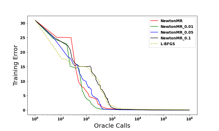
All algorithms are terminated when either the oracle calls reach $10^{6}$ , the magnitude of the gradient falls below $10^{-6}$ , or the step size/trust region goes below $10^{-18}$ . In the legends of Figures 1 and 2, ‘ $x\%$ ’ refers to when the approximate Hessian is formed using an ‘ $x$ ’ percent of the full dataset. For all other figures, ‘algorithm_ $x$ ’ refers to a given algorithm when $100x$ percent of the full dataset is used to construct the Hessian. When there is no postfix, the Hessian matrix is formed exactly.

4.2 Binary Classification

We first investigate the advantages/disadvantages of Hessian approximation within Newton-MR framework using two simple finite-sum problems in the form of binary classification. Namely, we consider convex binary logistic regression (Figure 1),

\displaystyle f(\mathbf{x})=\frac{1}{n}\sum_{i=1}^{n}\ln(1+\exp({\langle\mathbf{a}_{i},\mathbf{x}\rangle}))-b_{i}\langle\mathbf{a}_{i},\mathbf{x}\rangle,

and nonconvex nonlinear least square (Figure 2),

\displaystyle f(\mathbf{x})=\frac{1}{n}\sum_{i=1}^{n}\left(\frac{1}{1+\exp(-\langle\mathbf{a}_{i},\mathbf{x}\rangle)}-b_{i}\right)^{2}.

For our experiments here, we use the MINST data set [30], which contains of $60,000$ grayscale images of size $28\times 28$ , i.e., $\{(\mathbf{a}_{i},b_{i})\}_{i=1}^{n=60,000}\subset\mathbb{R}^{784}\times[0,1]$ . The labels of MNIST dataset are converted to binary classification, i.e., even and odd numbers.

In Algorithm 2, we set $\eta=0.001$ and $\mathbf{x}_{0}=\mathbf{0}$ . The results of running Algorithm 2 using various degrees of Hessian approximation are given in Figures 2 and 1. As predicted by our theory, Algorithm 2 converges irrespective of the degree of Hessian approximation. Also, while Hessian approximation generally helps with reducing the overall computational costs, its effectiveness can diminish if the approximation is overly crude. This is expected since a significant reduction in sub-sample size could lead to a substantial loss of curvature information, resulting in poor performance.

Refer to caption — Figure 1: Performance of Algorithm 2 using various degrees of Hessian approximation on the nonconvex nonlinear least squares loss function. As predicted by our theory, Algorithm 2 converges irrespective of the degree of Hessian approximation. Also, Hessian approximation typically reduces computational costs; however, a substantial reduction in sub-sample size can lead to a significant loss of curvature information, resulting in poor performances.

4.3 Feed Forward Neural Network

In this section, we consider a multi-class classification problem using a feed forward neural network, namely

f(\mathbf{x})=-\frac{1}{n}\left(\sum_{i=1}^{n}\left\langle\mathbf{b}_{i},\ln\left(\mathbf{h}(\mathbf{x};\mathbf{a}_{i})\right)\right\rangle\right)+\lambda g(\mathbf{x}),

(4.1)

where $\mathbf{h}(\mathbf{x};\mathbf{a}_{i}):\mathbb{R}^{d}\to[0,1]^{C}$ represent the output of the neural network, $\mathbf{b}_{i}\in\{0,1\}^{C}$ denotes the labels corresponding to input data $\mathbf{a}_{i}$ , $g(\mathbf{x}):\mathbb{R}^{d}\to\mathbb{R}$ is a nonconvex regularizer defined as $g(\mathbf{x})\triangleq\sum^{d}_{i=1}x_{i}^{2}/(1+x_{i}^{2})$ , and $\lambda>0$ is a regularization parameter.

We first consider CIFAR10 dataset [45], consisting of $60,000$ colored images of size $32\times 32$ in 10 classes, i.e., $\{(\mathbf{a}_{i},\mathbf{b}_{i})\}_{i=1}^{n=60,000}\subset\mathbb{R}^{3,072}\times\{0,1\}^{10}$ . We split the 60,000 samples into 50,000 training samples and 10,000 validation samples. Figures 3, 4 and 5 depict the performance of each algorithm on the training data. Plots showing performance in terms of validation accuracy/error are gathered in Section A.2. The feed forward neural network has the following architecture,

\displaystyle 3072\text{ (input)}\to\tanh\to 512\to\tanh\to 128\to\tanh\to 32\to\text{softmax}\to 10\text{ (output)},

resulting in $d=1,643,498$ numbers of parameters. The regularization parameter is set to $\lambda=10^{-8}$ . All algorithms are initialized from a normal distribution with zero mean and co-variance $0.1\mathbf{I}$ . The inexactness and the $\sigma$ -LC parameters of Algorithm 2 are set to $\eta=10$ and $\sigma=10^{-16}$ . For Newton-CG [67, 79], the desired accuracy for Capped-CG is set to $0.01$ .

Next, we consider a different dataset, namely Covertype [15], which includes $n=300,000$ training and $2,000$ validation samples of $54$ attributes across seven classes. Figures 7, 6 and 8 depict the performance of each algorithm on the training data. Plots showing performance in terms of validation accuracy/error are gathered in Section A.2. For these experiments, the neural network architecture is chosen to be

	$\displaystyle 54\text{ (input)}\to\text{sigmoid}\to 256\to\tanh\to 256\to\text{sigmoid}\to 128\to\tanh\to 128\to$
	$\displaystyle\to\text{sigmoid}\to 64\to\tanh\to 64\to\text{sigmoid}\to 32\to\tanh\to 32\to\text{softmax}\to 7\text{ (output)},$

resulting in $d=145,063$ . We also set $\lambda=10^{-8}$ . Again, $\mathbf{x}_{0}$ is chosen as above. For Newton-MR, the sub-problem inexactness and $\sigma$ -LC parameters are changed to $\eta=10,000$ and $\sigma=10^{-26}$ respectively. For Newton-CG, the desired accuracy parameter is set to $0.01$ .

In the experiments of this section, all algorithms reach the maximum allowed number of oracle calls. In all Figures 3, 4, 5, 7, 6 and 8, Algorithm 2 with appropriate degree of sub-sampling either is very competitive with, or downright superior to, alternative methods. Using the exact Hessian improves convergence by reducing the number of iterations. However, unless highly accurate solutions are required – which is often not necessary in machine learning applications – subsampling the Hessian can reduce the number of required oracle calls. What is striking is the relative poor performance of all Newton-CG variants. This further corroborates the observations in [65, 51, 52] that MINRES typically manifests itself as a far superior inner solver than the widely used CG method.

4.4 Recurrent Neural Network

Finally, we consider a slightly more challenging problem of training a recurrent neural network (RNN) [72] with mean squared error loss. Specifically, we consider the following objective function

\displaystyle f(\mathbf{x})=\frac{1}{n}\sum_{i=1}^{n}\left\|\mathbf{h}(\mathbf{x};\mathbf{a}_{i})-\mathbf{b}_{i}\right\|^{2}+\lambda g(\mathbf{x}),

where $\mathbf{h}(\mathbf{x};\mathbf{a})$ is the output of the RNN and $g(\mathbf{x})$ is again the same nonconvex regularizer as in Section 4.3 with regularization parameter $\lambda=10^{-8}$ . The point $\mathbf{x}_{0}$ is chosen in the same manner as in Section 4.3.

For the experiment here, we use the Gas sensor array under dynamic gas mixtures data set [36], which is a time series data. In particular, the data contains a time series of 16 features across three time stamps. So, we get $\{\mathbf{a}_{i},\mathbf{b}_{i}\}_{i=1}^{n=45,828}\subset(\mathbb{R}^{3}\times\mathbb{R}^{16})\times\mathbb{R}$ , and $d=100,417$ . We further split the samples into 40,828 training and 5,000 validation samples. For Newton-MR, the relative residual tolerance is set to $\eta=100$ . For Newton-CG, the accuracy of Capped-CG is set to $0.1$ .

Figures 9, 11 and 10 depict the performance of each algorithm on the training data. Plots showing performance in terms of validation accuracy/error are gathered in Section A.2. Once again, in all these experiments, Algorithm 2 with adequate sub-sampling can either outperform or at least remain competitive with the alternative methods. Also, one can again observe the visibly poor performance of Newton-CG relative to Algorithm 2. In Figure 9, $\texttt{NewtonCG}\_0.05$ and $\texttt{NewtonCG}\_0.1$ are terminated after 1410 and 2168 iterations, respectively, as their step sizes get below $10^{-18}$ . All the other algorithms reach the maximum allowed number of oracle calls.

5 Conclusion

We considered a variant of the Newton-MR algorithm for nonconvex problems, initially proposed in [51], to accommodate inexact Hessian information. Our primary focus was to establish iteration and operation complexities of our proposed variant under simple assumptions and with minimal algorithmic changes. In particular, we assume minimal smoothness on the gradient without extending it to the Hessian, and we avoid Hessian regularization/damping techniques to maintain curvature information and prevent performance degradation. We show that our algorithm converges regardless of the degree of approximation of the Hessian as well as the accuracy of the solution to the sub-problem. Beyond general nonconvex settings, we consider, in particular, a subclass of functions that satisfy the $\theta$ -PL condition and show that with $\theta=2$ , our algorithm achieves a global linear convergence rate while for $1\leq\theta<2$ , the global convergence transitions from a linear rate to a sub-linear rate in the neighbourhood of a solution. Finally, we provided numerical experiments on several machine learning problems to further illustrate the advantages of sub-sampled Hessian in the Newton-MR framework.

5.1 Acknowledgments

Fred Roosta was partially supported by the Australian Research Council through an Industrial Transformation Training Centre for Information Resilience (IC200100022) as well as a Discovery Early Career Researcher Award (DE180100923).

References

[1] Alekh Agarwal, Sham M Kakade, Jason D Lee, and Gaurav Mahajan. On the theory of policy gradient methods: Optimality, approximation, and distribution shift. Journal of Machine Learning Research, 22(98):1–76, 2021.
[2] Motasem Alfarra, Slavomir Hanzely, Alyazeed Albasyoni, Bernard Ghanem, and Peter Richtárik. Adaptive Learning of the Optimal Batch Size of SGD. arXiv preprint arXiv:2005.01097, 2020.
[3] Zeyuan Allen-Zhu, Yuanzhi Li, and Zhao Song. A convergence theory for deep learning via over-parameterization. In International conference on machine learning, pages 242–252. PMLR, 2019.
[4] Yossi Arjevani, Yair Carmon, John C Duchi, Dylan J Foster, Ayush Sekhari, and Karthik Sridharan. Second-order information in non-convex stochastic optimization: Power and limitations. In Conference on Learning Theory, pages 242–299. PMLR, 2020.
[5] Raef Bassily, Mikhail Belkin, and Siyuan Ma. On exponential convergence of SGD in non-convex over-parametrized learning. arXiv preprint arXiv:1811.02564, 2018.
[6] A. Beck. First-Order Methods in Optimization. MOS-SIAM Series on Optimization. Society for Industrial and Applied Mathematics, 2017.
[7] Stefania Bellavia, Eugenio Fabrizi, and Benedetta Morini. Linesearch Newton-CG methods for convex optimization with noise. ANNALI DELL’UNIVERSITA’DI FERRARA, 68(2):483–504, 2022.
[8] Stefania Bellavia and Gianmarco Gurioli. Stochastic analysis of an adaptive cubic regularization method under inexact gradient evaluations and dynamic Hessian accuracy. Optimization, 71(1):227–261, 2022.
[9] Stefania Bellavia, Gianmarco Gurioli, and Benedetta Morini. Adaptive cubic regularization methods with dynamic inexact Hessian information and applications to finite-sum minimization. IMA Journal of Numerical Analysis, 41(1):764–799, 2021.
[10] Stefania Bellavia, Nataša Krejić, and Nataša Krklec Jerinkić. Subsampled inexact Newton methods for minimizing large sums of convex functions. IMA Journal of Numerical Analysis, 40(4):2309–2341, 2020.
[11] Stefania Bellavia, Nataša Krejić, and Benedetta Morini. Inexact restoration with subsampled trust-region methods for finite-sum minimization. Computational Optimization and Applications, 76:701–736, 2020.
[12] Albert S Berahas, Raghu Bollapragada, and Jorge Nocedal. An investigation of Newton-sketch and subsampled Newton methods. Optimization Methods and Software, 35(4):661–680, 2020.
[13] El Houcine Bergou, Youssef Diouane, Vladimir Kunc, Vyacheslav Kungurtsev, and Clément W Royer. A subsampling line-search method with second-order results. INFORMS Journal on Optimization, 4(4):403–425, 2022.
[14] Dennis S Bernstein. Matrix mathematics: Theory, Facts, and Formulas (Second Edition). Princeton university press, 2009.
[15] Jock Blackard. Covertype. UCI Machine Learning Repository, 1998. DOI: https://doi.org/10.24432/C50K5N.
[16] Jose Blanchet, Coralia Cartis, Matt Menickelly, and Katya Scheinberg. Convergence rate analysis of a stochastic trust-region method via supermartingales. INFORMS journal on optimization, 1(2):92–119, 2019.
[17] Raghu Bollapragada, Richard H Byrd, and Jorge Nocedal. Exact and inexact subsampled Newton methods for optimization. IMA Journal of Numerical Analysis, 39(2):545–578, 2019.
[18] Richard H. Byrd, Gillian M. Chin, Will Neveitt, and Jorge Nocedal. On the use of stochastic Hessian information in optimization methods for machine learning. SIAM Journal on Optimization, 21(3):977–995, 2011.
[19] Richard H. Byrd, Gillian M. Chin, Jorge Nocedal, and Yuchen Wu. Sample size selection in optimization methods for machine learning. Mathematical programming, 134(1):127–155, 2012.
[20] Yair Carmon and John C Duchi. Analysis of Krylov subspace solutions of regularized non-convex quadratic problems. Advances in Neural Information Processing Systems, 31, 2018.
[21] Yair Carmon, John C Duchi, Oliver Hinder, and Aaron Sidford. “Convex until proven guilty”: dimension-free acceleration of gradient descent on non-convex functions. In International conference on machine learning, pages 654–663. PMLR, 2017.
[22] Coralia Cartis, Jaroslav Fowkes, and Zhen Shao. Randomised subspace methods for non-convex optimization, with applications to nonlinear least-squares. arXiv preprint arXiv:2211.09873, 2022.
[23] Coralia Cartis, Nicholas IM Gould, and Philippe L Toint. Adaptive cubic regularisation methods for unconstrained optimization. part i: motivation, convergence and numerical results. Mathematical Programming, 127(2):245–295, 2011.
[24] Coralia Cartis, Nicholas IM Gould, and Philippe L Toint. Adaptive cubic regularisation methods for unconstrained optimization. part ii: worst-case function-and derivative-evaluation complexity. Mathematical programming, 130(2):295–319, 2011.
[25] Coralia Cartis, Nicholas IM Gould, and Philippe L Toint. Worst-case evaluation complexity and optimality of second-order methods for nonconvex smooth optimization. In Proceedings of the International Congress of Mathematicians: Rio de Janeiro 2018, pages 3711–3750. World Scientific, 2018.
[26] Coralia Cartis, Nicholas IM Gould, and Philippe L Toint. Evaluation Complexity of Algorithms for Nonconvex Optimization: Theory, Computation and Perspectives. SIAM, 2022.
[27] Jiabin Chen, Rui Yuan, Guillaume Garrigos, and Robert M Gower. SAN: stochastic average newton algorithm for minimizing finite sums. In International Conference on Artificial Intelligence and Statistics, pages 279–318. PMLR, 2022.
[28] Andrew R Conn, Nicholas IM Gould, and Philippe L Toint. Trust region methods. SIAM, 2000.
[29] Frank E Curtis, Daniel P Robinson, Clément W Royer, and Stephen J Wright. Trust-region Newton-CG with strong second-order complexity guarantees for nonconvex optimization. SIAM Journal on Optimization, 31(1):518–544, 2021.
[30] Li Deng. The MNIST database of handwritten digit images for machine learning research [best of the web]. IEEE signal processing magazine, 29(6):141–142, 2012.
[31] Michał Dereziński and Elizaveta Rebrova. Sharp analysis of sketch-and-project methods via a connection to randomized singular value decomposition. SIAM Journal on Mathematics of Data Science, 6(1):127–153, 2024.
[32] John Duchi, Elad Hazan, and Yoram Singer. Adaptive subgradient methods for online learning and stochastic optimization. Journal of machine learning research, 12(7), 2011.
[33] Murat A Erdogdu and Andrea Montanari. Convergence rates of sub-sampled Newton methods. Advances in Neural Information Processing Systems, 28, 2015.
[34] Ilyas Fatkhullin, Jalal Etesami, Niao He, and Negar Kiyavash. Sharp analysis of stochastic optimization under global Kurdyka-Lojasiewicz inequality. Advances in Neural Information Processing Systems, 35:15836–15848, 2022.
[35] Zhili Feng, Fred Roosta, and David P Woodruff. Non-PSD matrix sketching with applications to regression and optimization. In Uncertainty in Artificial Intelligence, pages 1841–1851. PMLR, 2021.
[36] Jordi Fonollosa, Sadique Sheik, Ramón Huerta, and Santiago Marco. Reservoir computing compensates slow response of chemosensor arrays exposed to fast varying gas concentrations in continuous monitoring. Sensors and Actuators B: Chemical, 215:618–629, 2015.
[37] Terunari Fuji, Pierre-Louis Poirion, and Akiko Takeda. Randomized subspace regularized Newton method for unconstrained non-convex optimization. arXiv preprint arXiv:2209.04170, 2022.
[38] Ian Goodfellow, Yoshua Bengio, and Aaron Courville. Deep learning. MIT press, 2016.
[39] Nicholas IM Gould, Stefano Lucidi, Massimo Roma, and Ph L Toint. Exploiting negative curvature directions in linesearch methods for unconstrained optimization. Optimization methods and software, 14(1-2):75–98, 2000.
[40] Robert Gower, Dmitry Kovalev, Felix Lieder, and Peter Richtárik. RSN: Randomized subspace Newton. Advances in Neural Information Processing Systems, 32, 2019.
[41] Serge Gratton, Clément W Royer, Luís N Vicente, and Zaikun Zhang. Complexity and global rates of trust-region methods based on probabilistic models. IMA Journal of Numerical Analysis, 38(3):1579–1597, 2018.
[42] Billy Jin, Katya Scheinberg, and Miaolan Xie. Sample complexity analysis for adaptive optimization algorithms with stochastic oracles. Mathematical Programming, pages 1–29, 2024.
[43] Hamed Karimi, Julie Nutini, and Mark Schmidt. Linear convergence of gradient and proximal-gradient methods under the polyak-łojasiewicz condition. In Machine Learning and Knowledge Discovery in Databases: European Conference, ECML PKDD 2016, Riva del Garda, Italy, September 19-23, 2016, Proceedings, Part I 16, pages 795–811. Springer, 2016.
[44] Diederik P Kingma and Jimmy Ba. Adam: A method for stochastic optimization. arXiv preprint arXiv:1412.6980, 2014.
[45] Alex Krizhevsky, Geoffrey Hinton, et al. Learning multiple layers of features from tiny images. Technical Report, 2009.
[46] G. Lan. First-order and Stochastic Optimization Methods for Machine Learning. Springer Series in the Data Sciences. Springer International Publishing, 2020.
[47] Kenneth Levenberg. A method for the solution of certain non-linear problems in least squares. Quarterly of applied mathematics, 2(2):164–168, 1944.
[48] Shuyao Li and Stephen J Wright. A randomized algorithm for nonconvex minimization with inexact evaluations and complexity guarantees. arXiv preprint arXiv:2310.18841, 2023.
[49] Alexander Lim, Yang Liu, and Fred Roosta. Conjugate Direction Methods Under Inconsistent Systems. arXiv preprint arXiv:2401.11714, 2024.
[50] Z. Lin, H. Li, and C. Fang. Accelerated Optimization for Machine Learning: First-Order Algorithms. Springer Singapore, 2020.
[51] Yang Liu and Fred Roosta. Convergence of Newton-MR under inexact Hessian information. SIAM Journal on Optimization, 31(1):59–90, 2021.
[52] Yang Liu and Fred Roosta. A Newton-MR algorithm with complexity guarantees for nonconvex smooth unconstrained optimization. arXiv preprint arXiv:2208.07095, 2022.
[53] Yang Liu and Fred Roosta. MINRES: From Negative Curvature Detection to Monotonicity Properties. SIAM Journal on Optimization, 32(4):2636–2661, 2022.
[54] Ilya Loshchilov and Frank Hutter. Decoupled weight decay regularization. arXiv preprint arXiv:1711.05101, 2017.
[55] Donald W Marquardt. An algorithm for least-squares estimation of nonlinear parameters. Journal of the society for Industrial and Applied Mathematics, 11(2):431–441, 1963.
[56] Jincheng Mei, Chenjun Xiao, Csaba Szepesvari, and Dale Schuurmans. On the global convergence rates of softmax policy gradient methods. In International conference on machine learning, pages 6820–6829. PMLR, 2020.
[57] Shashi K Mishra and Giorgio Giorgi. Invexity and optimization, volume 88. Springer Science & Business Media, 2008.
[58] Sen Na, Michał Dereziński, and Michael W Mahoney. Hessian averaging in stochastic Newton methods achieves superlinear convergence. Mathematical Programming, 201(1):473–520, 2023.
[59] Sen Na and Michael W. Mahoney. Statistical Inference of Constrained Stochastic Optimization via Sketched Sequential Quadratic Programming. arXiv preprint arXiv:2205.13687, 2024.
[60] Yurii Nesterov and Boris T Polyak. Cubic regularization of Newton method and its global performance. Mathematical Programming, 108(1):177–205, 2006.
[61] Jorge Nocedal and Stephen Wright. Numerical optimization. Springer Science & Business Media, 2006.
[62] Christopher C Paige and Michael A Saunders. Solution of sparse indefinite systems of linear equations. SIAM journal on numerical analysis, 12(4):617–629, 1975.
[63] Mert Pilanci and Martin J Wainwright. Newton sketch: A near linear-time optimization algorithm with linear-quadratic convergence. SIAM Journal on Optimization, 27(1):205–245, 2017.
[64] Francesco Rinaldi, Luis Nunes Vicente, and Damiano Zeffiro. Stochastic trust-region and direct-search methods: A weak tail bound condition and reduced sample sizing. SIAM Journal on Optimization, 34(2):2067–2092, 2024.
[65] Fred Roosta, Yang Liu, Peng Xu, and Michael W Mahoney. Newton-MR: Inexact Newton method with minimum residual sub-problem solver. EURO Journal on Computational Optimization, 10:100035, 2022.
[66] Farbod Roosta-Khorasani and Michael W Mahoney. Sub-sampled Newton methods. Mathematical Programming, 174(1):293–326, 2019.
[67] Clément W Royer, Michael O’Neill, and Stephen J Wright. A Newton-CG algorithm with complexity guarantees for smooth unconstrained optimization. Mathematical Programming, 180:451–488, 2020.
[68] Clément W Royer and Stephen J Wright. Complexity analysis of second-order line-search algorithms for smooth nonconvex optimization. SIAM Journal on Optimization, 28(2):1448–1477, 2018.
[69] Sebastian Ruder. An overview of gradient descent optimization algorithms. arXiv preprint arXiv:1609.04747, 2016.
[70] Yousef Saad. Iterative methods for sparse linear systems. SIAM, 2003.
[71] Shai Shalev-Shwartz and Shai Ben-David. Understanding machine learning: From theory to algorithms. Cambridge university press, 2014.
[72] Alex Sherstinsky. Fundamentals of recurrent neural network (rnn) and long short-term memory (lstm) network. Physica D: Nonlinear Phenomena, 404:132306, 2020.
[73] Yingjie Tian, Yuqi Zhang, and Haibin Zhang. Recent advances in stochastic gradient descent in deep learning. Mathematics, 11(3):682, 2023.
[74] Nilesh Tripuraneni, Mitchell Stern, Chi Jin, Jeffrey Regier, and Michael I Jordan. Stochastic cubic regularization for fast nonconvex optimization. Advances in neural information processing systems, 31, 2018.
[75] Peng Xu, Fred Roosta, and Michael W Mahoney. Newton-type methods for non-convex optimization under inexact hessian information. Mathematical Programming, 184(1-2):35–70, 2020.
[76] Peng Xu, Fred Roosta, and Michael W Mahoney. Second-order optimization for non-convex machine learning: An empirical study. In Proceedings of the 2020 SIAM International Conference on Data Mining, pages 199–207. SIAM, 2020.
[77] Peng Xu, Jiyan Yang, Fred Roosta, Christopher Ré, and Michael W Mahoney. Sub-sampled Newton methods with non-uniform sampling. In Advances in Neural Information Processing Systems (NeurIPS-16), pages 3000–3008, 2016.
[78] Zhewei Yao, Peng Xu, Fred Roosta, and Michael W Mahoney. Inexact nonconvex Newton-type methods. INFORMS Journal on Optimization, 3(2):154–182, 2021.
[79] Zhewei Yao, Peng Xu, Fred Roosta, Stephen J Wright, and Michael W Mahoney. Inexact Newton-CG algorithms with complexity guarantees. IMA Journal of Numerical Analysis, 43(3):1855–1897, 2023.
[80] Rui Yuan, Robert M Gower, and Alessandro Lazaric. A general sample complexity analysis of vanilla policy gradient. In International Conference on Artificial Intelligence and Statistics, pages 3332–3380. PMLR, 2022.
[81] Rui Yuan, Alessandro Lazaric, and Robert M Gower. Sketched Newton–Raphson. SIAM Journal on Optimization, 32(3):1555–1583, 2022.
[82] Matthew D Zeiler. Adadelta: an adaptive learning rate method. arXiv preprint arXiv:1212.5701, 2012.
[83] Jinshan Zeng, Shikang Ouyang, Tim Tsz-Kit Lau, Shaobo Lin, and Yuan Yao. Global convergence in deep learning with variable splitting via the Kurdyka-Łojasiewicz property. arXiv preprint arXiv:1803.00225, 9, 2018.

Appendix A Appendix

A.1 Proof of 1

The results have been established, in one form or another, in prior works [70, 53]; however we provide the proofs here for the sake of completeness. The proofs of 2.1 and 2.2 can be readily found in [70] and [53, Lemma 3.1d] respectively. For 2.3, we note $\langle\mathbf{r}^{(t-1)},\mathbf{r}^{(i)}\rangle=\langle\mathbf{r}^{(t-1)},-\mathbf{g}-\mathbf{\bar{H}}\mathbf{s}^{(i)}\rangle=\|\mathbf{r}^{(t-1)}\|^{2}$ , where the last equality follows from 2.2 and Petrov-Galerkin condition, i.e., $\mathbf{r}^{(t-1)}\perp\mathbf{\bar{H}}\mathcal{K}_{t}({\mathbf{\bar{H}}},{\mathbf{g}})$ . Property 2.4 can be found in [53, Theorem 3.8a]. For 2.5, the increasing sequence $\|\mathbf{s}^{(i)}\|\geq\|\mathbf{s}^{(j)}\|$ can be again found in [53, Theorem 3.11e]. For the expression of $\mathbf{s}^{(1)}$ , we write

\displaystyle\mathbf{s}^{(1)}=\underset{\mathbf{s}\in\mathcal{K}_{1}({\mathbf{\bar{H}}},{\mathbf{g}})}{\text{argmin}}\left\|-\mathbf{g}-\mathbf{\bar{H}}\mathbf{s}\right\|^{2}=\underset{\mathbf{s}\in\text{span}(\mathbf{g})}{\text{argmin}}\left\|\mathbf{\bar{H}}\mathbf{s}\right\|^{2}+2\left\langle{\mathbf{g},\mathbf{\bar{H}}\mathbf{s}}\right\rangle

So, the vector $\mathbf{s}^{(1)}$ must be some multiple of $\mathbf{g}$ , i.e., $\mathbf{s}^{(1)}=\alpha\mathbf{g}$ . To find $\alpha$ , we note,

\displaystyle\frac{\left\langle{\mathbf{g},\mathbf{\bar{H}}\mathbf{g}}\right\rangle}{\left\|\mathbf{\bar{H}}\mathbf{g}\right\|^{2}}=\underset{\alpha\in\mathbb{R}}{\text{argmin}}\,\,\alpha^{2}\left\|\mathbf{\bar{H}}\mathbf{g}\right\|^{2}+2\alpha\left\langle{\mathbf{g},\mathbf{\bar{H}}\mathbf{g}}\right\rangle.

A.2 Further Numerical Results: Training and Validation Accuracy/Error

In this section, we provide the comparative performance of all methods, as measured by training and validation accuracy/error in each experiment of Section 4.

A.3 Why not damp/regularize the Hessian matrix?

As mentioned earlier, our primary focus in this paper is to design a convergent algorithm for nonconvex problems that requires minimal algorithmic modification, relative to similar Newton-type methods in the literature. In nonconvex settings, many Newton-type methods often consider some modifications to the Hessian, e.g. Levenberg-Marquardt [47, 55], Newton-CG [67, 75], and Trust-region-CG [29]. In particular, the regularized/damped Hessian in the form of $\tilde{\mathbf{H}}_{k}=\mathbf{H}_{k}+\zeta\mathbf{I}$ , for some $\zeta>0$ , is used in [67, 75, 29] within the Capped-CG procedure. Not only does this particular modification allow for the extraction of sufficiently negative curvature direction, but it also provides a means for obtaining state-of-the-art convergent analysis. However, as we now show, this damping of the Hessian spectrum can adversely affect the practical performance of the algorithm. Figure 21 depicts the results of the nonlinear least square problem from Section 4.2 with CIFAR10 dataset [45]. We consider different magnitudes of damping for the Hessian. As it can be seen, almost always, such a regularization/damping results in poor empirical performance. Intuitively, this is largely due to the lessening the contribution of the eigenvectors corresponding to the small eigenvalues of the Hessian in forming the update direction.

	$\displaystyle\sigma d\left\\|(\mathbf{VV}^{\top}-\mathbf{V}_{j}\mathbf{V}_{j}^{\top})\mathbf{g}\right\\|^{2}$	$\displaystyle+\sigma d\left\\|\mathbf{V}_{j}\mathbf{V}_{j}^{\top}\mathbf{g}\right\\|^{2}+\sigma d\left\\|\mathbf{V}_{\perp}\mathbf{V}_{\perp}^{\top}\mathbf{g}\right\\|^{2}$
		$\displaystyle<\left\langle{\mathbf{V}_{j}\mathbf{V}_{j}^{\top}\mathbf{g},\mathbf{\bar{H}}\mathbf{V}_{j}\mathbf{V}_{j}^{\top}\mathbf{g}}\right\rangle+\left\langle{(\mathbf{VV}^{\top}-\mathbf{V}_{j}\mathbf{V}_{j}^{\top})\mathbf{g},\mathbf{\bar{H}}(\mathbf{VV}^{\top}-\mathbf{V}_{j}\mathbf{V}_{j}^{\top})\mathbf{g}}\right\rangle$
		$\displaystyle\leq(L_{\mathbf{g}}+\varepsilon)\left\\|\mathbf{V}_{j}\mathbf{V}_{j}^{\top}\mathbf{g}\right\\|^{2}+\frac{\sigma d}{2}\left\\|(\mathbf{VV}^{\top}-\mathbf{V}_{j}\mathbf{V}_{j}^{\top})\mathbf{g}\right\\|^{2},$

	$\displaystyle\left\\|\mathbf{r}^{(t)}\right\\|^{2}$	$\displaystyle=\min_{\mathbf{s}\in\mathcal{K}_{t}(\mathbf{\bar{H}},\mathbf{g})}\left\\|\mathbf{\bar{H}}\mathbf{s}+\mathbf{g}\right\\|^{2}$
		$\displaystyle=\min_{\mathbf{s}\in\mathbf{V}_{i}\mathbf{V}_{i}^{\top}\mathcal{K}_{t}(\mathbf{\bar{H}},\mathbf{g})}\left\\|\mathbf{\bar{H}}\mathbf{s}+\mathbf{V}_{i}\mathbf{V}_{i}^{\top}\mathbf{g}\right\\|^{2}+\min_{\mathbf{s}\in(\mathbf{V}_{i\perp}\mathbf{V}_{i\perp}^{\top}+\mathbf{V}_{\perp}\mathbf{V}_{\perp}^{\top})\mathcal{K}_{t}(\mathbf{\bar{H}},\mathbf{g})}\left\\|\mathbf{\bar{H}}\mathbf{s}+(\mathbf{V}_{i\perp}\mathbf{V}_{i\perp}^{\top}+\mathbf{V}_{\perp}\mathbf{V}_{\perp}^{\top})\mathbf{g}\right\\|^{2}$
		$\displaystyle=\min_{\mathbf{s}\in\mathbf{V}_{i}\mathbf{V}_{i}^{\top}\mathcal{K}_{t}(\mathbf{\bar{H}},\mathbf{g})}\left\\|\mathbf{\bar{H}}\mathbf{s}+\mathbf{V}_{i}\mathbf{V}_{i}^{\top}\mathbf{g}\right\\|^{2}+\min_{\mathbf{s}\in\mathbf{V}_{i\perp}\mathbf{V}_{i\perp}^{\top}\mathcal{K}_{t}(\mathbf{\bar{H}},\mathbf{g})}\left\\|\mathbf{\bar{H}}\mathbf{s}+\mathbf{V}_{i\perp}\mathbf{V}_{i\perp}^{\top}\mathbf{g}\right\\|^{2},$

Complexity Guarantees for Nonconvex Newton-MR Under Inexact Hessian Information

Abstract

keywords:

1 Introduction

Notation

Definitions

Definition 1 (θ\theta-Polyak-Łojasiewicz Condition).

Definition 2 (εf\varepsilon_{f}-Global Optimality).

Definition 3 (ε𝐠\varepsilon_{\mathbf{g}}-First Order Optimality).

Definition 4 (σ\sigma-Limited Curvature Direction).

Definition 5 (Inexact Hessian).

2 Newton-MR with Inexact Hessian

Condition 1 (Sub-problem Inexactness Condition).

Condition 2 (σ\sigma-Limited Curvature Condition).

Lemma 1.

Proof.

Properties 1.

3 Theoretical Analyses

Assumption 1.

3.1 Iteration Complexity

Lemma 2.

Proof.

Lemma 3.

Proof.

Theorem 1.

Proof.

Remark 1.

Remark 2.

Remark 3.

3.2 Operation Complexity

Definition 6.

Example 1.

Lemma 4.

Proof.

Lemma 5.

Proof.

Lemma 6.

Proof.

Corollary 1 (Optimal Operation Complexity of Algorithm 2).

4 Numerical Experiments

4.1 Implementation details

Newton-MR and its sub-sampled variants

Newton-CG and its sub-sampled variants

Steihaug’s trust-region and its sub-sampled variants

L-BFGS

4.2 Binary Classification

4.3 Feed Forward Neural Network

4.4 Recurrent Neural Network

5 Conclusion

5.1 Acknowledgments

References

Appendix A Appendix

A.1 Proof of 1

A.2 Further Numerical Results: Training and Validation Accuracy/Error

A.3 Why not damp/regularize the Hessian matrix?

Definition 1 ( $\theta$ -Polyak-Łojasiewicz Condition).

Definition 2 ( $\varepsilon_{f}$ -Global Optimality).

Definition 3 ( $\varepsilon_{\mathbf{g}}$ -First Order Optimality).

Definition 4 ( $\sigma$ -Limited Curvature Direction).

Condition 2 ( $\sigma$ -Limited Curvature Condition).