Complex matrix inversion via real matrix inversions

Zhen Dai , Lek-Heng Lim Computational and Applied Mathematics Initiative, University of Chicago, Chicago, IL 60637-1514 [email protected], [email protected] and Ke Ye KLMM, Academy of Mathematics and Systems Science, Chinese Academy of Sciences, Beijing 100190, China [email protected]

Abstract.

We study the inversion analog of the well-known Gauss algorithm for multiplying complex matrices. A simple version is $(A+iB)^{-1}=(A+BA^{-1}B)^{-1}-iA^{-1}B(A+BA^{-1}B)^{-1}$ when $A$ is invertible, which may be traced back to Frobenius but has received scant attention. We prove that it is optimal, requiring fewest matrix multiplications and inversions over the base field, and we extend it in three ways: (i) to any invertible $A+iB$ without requiring $A$ or $B$ be invertible; (ii) to any iterated quadratic extension fields, with $\mathbb{C}$ over $\mathbb{R}$ a special case; (iii) to Hermitian positive definite matrices $A+iB$ by exploiting symmetric positive definiteness of $A$ and $A+BA^{-1}B$ . We call all such algorithms Frobenius inversions, which we will see do not follow from Sherman–Morrison–Woodbury type identities and cannot be extended to Moore–Penrose pseudoinverse. We show that a complex matrix with well-conditioned real and imaginary parts can be arbitrarily ill-conditioned, a situation tailor-made for Frobenius inversion. We prove that Frobenius inversion for complex matrices is faster than standard inversion by LU decomposition and Frobenius inversion for Hermitian positive definite matrices is faster than standard inversion by Cholesky decomposition. We provide extensive numerical experiments, applying Frobenius inversion to solve linear systems, evaluate matrix sign function, solve Sylvester equation, and compute polar decomposition, showing that Frobenius inversion can be more efficient than LU/Cholesky decomposition with negligible loss in accuracy. A side result is a generalization of Gauss multiplication to iterated quadratic extensions, which we show is intimately related to the Karatsuba algorithm for fast integer multiplication and multidimensional fast Fourier transform.

1. Introduction

The article is a sequel to our recent work in [14], where we studied the celebrated Gauss multiplication algorithm $(A+iB)(C+iD)=(AC-BD)+i[(A+B)(C+D)-AC-BD]$ for multiplying a pair of complex matrices with just three real matrix multiplications. Such methods for performing a complex matrix operation in terms of real matrix operations can be very useful as floating point standards such as the IEEE-754 [1] often do not implement complex arithmetic natively but rely on software to reduce complex arithmetic to real arithmetic [55, p. 55]. Here we will analyze and extend an inversion analogue of Gauss algorithm: Given a complex invertible matrix $A+iB\in\mathbb{C}^{n\times n}$ with $A,B\in\mathbb{R}^{n\times n}$ , it is straightforward to verify that its inverse is given by

(A+iB)^{-1}=(A+BA^{-1}B)^{-1}-iA^{-1}B(A+BA^{-1}B)^{-1}

(1)

if $A$ is invertible, a formula that can be traced back to Georg Frobenius [67]. In our article we will refer to all such algorithms and their variants and extensions as Frobenius inversions. While Gauss multiplication has been thoroughly studied (two representative references are [41, Section 4.6.4] in Computer Science and [32, Section 23.2.4] in Numerical Analysis, with numerous additional references therein), the same cannot be said of Frobenius inversion — we combed through the research literature and found only six references, all from the 1970s or earlier, which we will review in Section 1.3.

Our goal is to vastly extend and thoroughly analyze Frobenius inversion from a modern perspective. We will extend it to the general case where only $A+iB$ is invertible but neither $A$ nor $B$ is (Section 4.2), and to the important special case where $A+iB$ is Hermitian positive definite, in a way that exploits the symmetric positive definiteness of $A$ and $A+BA^{-1}B$ (Section 4.3). We will show (Section 3) that it is easy to find complex matrices $A+iB$ with

\max\bigl{(}\kappa_{2}(A),\kappa_{2}(B),\kappa_{2}(A+BA^{-1}B)\bigr{)}\ll\kappa_{2}(A+iB),

(2)

where the gap between the left- and right-hand side is arbitrarily large, i.e., $A+iB$ can be arbitrarily ill-conditioned even when $A,B,A+BA^{-1}B$ are all well-conditioned — a scenario bespoke for (1).

Frobenius inversion obviously extends to any quadratic fields of the form $\Bbbk[\sqrt{a}]$ , i.e., $x^{2}+a$ is irreducible over $\Bbbk$ , but we will further extend it to any arbitrary quadratic field, and any iterated quadratic extensions including constructible numbers, multiquadratics, and towers of root extensions (Section 2.4). In fact we show that for iterated quadratic extensions, Frobenius inversion essentially gives the multidimensional fast Fourier transform. We will prove that over any quadratic field Frobenius inversion is optimal in that it requires the least number of matrix multiplications and inversions over its base field (Sections 2.3, 4.3, and 4.2).

For complex matrix inversion, we show that Matlab’s built-in inversion algorithm, i.e., directly inverting a matrix with LU or Cholesky decomposition in complex arithmetic, is slower than applying Frobenius inversion with LU or Cholesky decomposition in real arithmetic (Theorem 4.1, Propositions 4.2 and 4.6). More importantly, we provide a series of numerical experiments in Section 5 to show that Frobenius inversion is indeed faster than Matlab’s built-in inversion algorithm in almost every situation and, despite well-known exhortations to avoid matrix inversion, suffers from no significant loss in accuracy. In fact methods based on Frobenius inversion may be more accurate than standard methods in certain scenarios (Section 5.2).

1.1. Why not invert matrices

Matrix inversion is frown upon in numerical linear algebra, likely an important cause for the lack of interest in algorithms like Frobenius inversion. The usual reason for eschewing inversion [34] is that in solving an $n\times n$ nonsingular system $Ax=b$ , if we compute a solution $\widehat{x}_{\operatorname{\mathsf{inv}}}$ by inverting $A$ through LU factorization $PA=LU$ and multiplying $A^{-1}$ to $b$ , and if we compute a solution $\widehat{x}_{LU}$ directly through the LU factors with backward substitutions $Ly=Pb$ , $Ux=y$ , the latter approach is both faster, with $2n^{3}$ flops for $\widehat{x}_{\operatorname{\mathsf{inv}}}$ versus $2n^{3}/3$ for $\widehat{x}_{LU}$ , and more accurate, with backward errors

\lvert b-A\widehat{x}_{\operatorname{\mathsf{inv}}}\rvert\leq n\lvert A\rvert\lvert A^{-1}\rvert\lvert b\rvert\mathsf{u}+O(\mathsf{u}^{2})\quad\text{versus}\quad\lvert b-A\widehat{x}_{LU}\rvert\leq 3n\lvert\widehat{L}\rvert\lvert\widehat{U}\rvert\lvert\widehat{x}_{LU}\rvert\mathsf{u}+O(\mathsf{u}^{2}).

(3)

Here $\mathsf{u}$ denotes unit roundoff and where $|\cdot|$ and $\leq$ applies componentwise. As noted in [34], usually $\lVert|\widehat{L}||\widehat{U}|\rVert_{\infty}\approx\lVert A\rVert_{\infty}$ and so $\widehat{x}_{LU}$ is likely more accurate than $\widehat{x}_{\operatorname{\mathsf{inv}}}$ when $\lVert x\rVert_{\infty}\ll\lVert|A^{-1}||b|\rVert_{\infty}$ .

Another common rationale for avoiding inversion is the old wisdom that many tasks that appear to require inversion actually do not — an explicit inverse matrix $A^{-1}\in\mathbb{C}^{n\times n}$ is almost never required because upon careful examination, one would invariably realize that the same objective could be accomplished with a vector like $A^{-1}b$ or $\operatorname{diag}(A^{-1})\in\mathbb{C}^{n}$ or a scalar like $c^{\scriptscriptstyle\mathsf{T}}A^{-1}b$ , $\lVert A^{-1}\rVert$ , or $\operatorname{tr}(A^{-1})\in\mathbb{C}$ . These vectors and scalars could be computed with a matrix factorization or approximated to arbitrary accuracy with iterative methods [28], which are often more amenable to updating/downdating [27] or better suited for preserving structures like sparsity.

Caveat

We emphasize that Frobenius inversion, when applied to solve a system of complex linear equations $(A+iB)z=c+id$ , will not involve actually computing an explicit inverse matrix $(A+iB)^{-1}$ and then multiplying it to the vector $c+id$ . In other words, we do not use the expression in (1) literally but only apply it in conjunction with various LU decompositions and back substitutions over $\mathbb{R}$ ; the matrix $(A+iB)^{-1}$ is never explicitly formed. The details are given in Section 3 alongside discussions of circumstances like (2) where the use of Frobenius inversion gives more accurate results than standard methods, with numerical evidence in Section 5.2.

1.2. Why invert matrices

We do not dispute the reasons in Section 1.1 but numerical linear algebra is a field that benefits from a wide variety of different methods for the same task, each suitable for a different regime. There is no single method that is universally best in every instance. Even the normal equation, frown upon in numerical linear algebra like matrix inversion, can be the ideal method for certain least squares problems.

In fact, if we examine the advantages of computing $\widehat{x}_{LU}$ over $\widehat{x}_{\operatorname{\mathsf{inv}}}$ in Section 1.1 more closely, we will find that the conclusion is not so clear cut. Firstly, the comparison in (3) assumes that accuracy is quantified by backward error $\lvert b-A\widehat{x}\rvert$ but in reality it is the forward error $\lvert x-\widehat{x}\rvert$ that is far more important and investigations in [15, 16], both analytical and experimental, show that the forward errors of $\widehat{x}_{LU}$ and $\widehat{x}_{\operatorname{\mathsf{inv}}}$ are similar. Secondly, if instead of solving a single linear system $Ax=b$ , we have $p$ right-hand sides $b_{1},\dots,b_{p}\in\mathbb{C}^{n}$ , then it becomes $AX=B$ where $B=[b_{1},\dots,b_{p}]\in\mathbb{C}^{n\times p}$ and we seek a solution $X\in\mathbb{C}^{n\times p}$ . In this case the speed advantage of computing $\widehat{X}_{LU}$ over $\widehat{X}_{\operatorname{\mathsf{inv}}}$ disappears when $p=O(n)$ : Note that the earlier flop count $2n^{3}/3$ for $\widehat{x}_{LU}$ ignores the cost of two backsubstitutions but when there are $2p$ backsubstitutions, these may no longer be ignored and are in fact dominant, making the cost of computing $\widehat{X}_{\operatorname{\mathsf{inv}}}$ and $\widehat{X}_{LU}$ comparable. In [15], it is shown that because of data structure complications, computing $\widehat{X}_{\operatorname{\mathsf{inv}}}$ can be significantly faster than $\widehat{X}_{LU}$ .

Moreover, the old wisdom that one may avoid computing explicit inverse matrices, while largely true, is not always true. There are situations, some of them alluded to in [34, p. 260], where computing an explicit inverse matrix is inevitable or favorable:

Mimo radios:: In such radios, explicit inverse matrices are implemented in hardware [16, 19, 66]. It is straightforward to hardwire or hardcode an explicit inverse matrix but considerably more difficult to do so in the form of “LU factors with permutations and backsubstitutions,” which can require more gates or code space and is more prone to implementation errors.
Superconductivity:: In the so-called KKR CPA algorithm [30], one needs to integrate the KKR inverse matrix over the first Brillouin zone, necessitating an explicit inverse matrix.
Linear modeling:: The inverse of a matrix often reveals important statistical properties that could only be discerned when one has access to the full explicit inverse [47, 48], i.e., we do not know which entries of $A^{-1}$ matter until we see all of them. For a specific example, take the ubiquitous model $y=X\widehat{\beta}+\varepsilon$ with design matrix $X$ and observed values $y_{1},\dots,y_{n}$ of the dependent variable $y$ [48], we understand the regression coefficients $\widehat{\beta}$ through the values its covariance matrix $\Sigma\coloneqq\sigma^{2}\cdot(X^{\scriptscriptstyle\mathsf{T}}X)^{-1}$ where $\sigma^{2}$ is the variance of the dependent variable [48]. To see which values are large (positively correlated), small (negatively correlated), or nearly zero (uncorrelated) in relation to other values, we need access to all values of $\Sigma$ .
Statistics:: For an unbiased estimator $\widehat{\theta}(X)$ of a parameter $\theta$ , its Cramer–Rao lower bound is the inverse of its Fisher information matrix $I(\theta)$ . This is an important quantity that gives a lower bound for the covariance matrix [13, 58] in the sense of $\operatorname{cov}_{\theta}\bigl{(}\widehat{\theta}(X)\bigr{)}\succeq I(\theta)^{-1}$ where $\succeq$ is the Loewner order. In some Gaussian processes, this lower bound could be attained [40]. We need the explicit matrix inverse $I(\theta)^{-1}$ to understand the limits of certain statistical problems and to design optimal estimators that attain the Cramer–Rao lower bound.
Graph theory:: The inverses of the adjacency matrix, forward adjacency matrix, and various graph Laplacians of a graph $G$ contain important combinatorial properties about $G$ [53, 56, 57, 69] that are only revealed when one examines all entries of their explicit inverse matrices.
Symbolic computing:: Matrix inversions do not just arise in numerical computing with floating point operations. They are routinely performed in finite field arithmetic over a base field of the form $\Bbbk=\operatorname{GF}(p^{n})$ in cryptography [36, 65], combinatorics [42], information theory [2], and finite field matrix computations [10]. They are also carried out in rational arithmetic over transcendental fields [20, 21, 26], e.g., with a base field of the form $\Bbbk=\mathbb{Q}(x_{1},\dots,x_{n},e^{x_{1}},\dots,e^{x_{n}})$ and an extension field of the form $\mathbb{F}=\mathbb{Q}[i](x_{1},\dots,x_{n},e^{x_{1}},\dots,e^{x_{n}})$ , or with finite fields in place of $\mathbb{Q}$ and $\mathbb{Q}[i]$ . With such exact arithmetic, the considerations in Section 1.1 become irrelevant.

In summary, the Frobenius inversion algorithms in this article are useful (i) for problems with well-conditioned $A$ , $B$ , and $A+BA^{-1}B$ but ill-conditioned $A+iB$ ; (ii) in situations requiring an explicit inverse matrix; (iii) to applications involving exact finite field or rational arithmetic.

1.3. Previous works

We review existing works that mentioned the inversion formula (1) in the research literature: [22, 23, 62, 64, 67, 70] — we note that this is an exhaustive list, and all predate 1979. We also widened our search to books and the education literature, and found [17, 46] in engineering education publications, [7, pp. 218–219], [32, Exercise 14.8], and [43, Chapter II, Section 20], although they contain no new material.

The algorithm, according to [67], was first discovered by Frobenius and Schur although we are unable to find a published record in their Collected Works [25, 61]. Since “Schur inversion” is already used to mean something unconnected to complex matrices, and calling (1) “Frobenius–Schur inversion” might lead to unintended confusion with Schur inversion, it seems befitting to name (1) after Frobenius alone.

The discussions in [22, 62, 70] are all about deriving Frobenius inversion. From a modern perspective, the key to these derivations is an embedding of $\mathbb{C}^{n\times n}$ into $\mathbb{R}^{2n\times 2n}$ as a subalgebra via

A+iB\mapsto\begin{bmatrix}A&-B\\ B&A\end{bmatrix}\eqqcolon M,

and noting that if $A$ is invertible, then $(A+iB)^{-1}$ corresponds to $M^{-1}$ , given by the standard expression

M^{-1}=\begin{bmatrix}A^{-1}-A^{-1}B(M/A)^{-1}BA^{-1}&A^{-1}B(M/A)^{-1}\\ -(M/A)^{-1}BA^{-1}&(M/A)^{-1}\end{bmatrix},

where $M/A\coloneqq A+BA^{-1}B$ denotes the Schur complement of $A$ in $M$ . The two right blocks of $M^{-1}$ then yield the expression

(A+iB)^{-1}=(M/A)^{-1}-iA^{-1}B(M/A)^{-1},

which is (1). The works in [43, 64] go further in addressing the case when both $A$ and $B$ are singular [43] and the case when $A$ , $B$ , $A+B$ or $A-B$ are all singular [64]. However, they require the inversion of a $2n\times 2n$ real matrix, wiping out any computational savings that Frobenius inversion affords. The works [23, 70] avoided this pitfall but still compromised the computational savings of Frobenius inversion. Our method in Section 4.2 will cover these cases and more, all while preserving the computational complexity of Frobenius inversion.

1.4. Notations and conventions

Fields are denoted in blackboard bold fonts. We write

	$\displaystyle\operatorname{GL}_{n}(\mathbb{F})$	$\displaystyle\coloneqq\{X\in\mathbb{F}^{n\times n}:\det(X)\neq 0\},$
	$\displaystyle\operatorname{O}_{n}(\mathbb{R})$	$\displaystyle\coloneqq\{X\in\mathbb{R}^{n\times n}:X^{\scriptscriptstyle\mathsf{T}}X=I\},$
	$\displaystyle\operatorname{U}_{n}(\mathbb{C})$	$\displaystyle\coloneqq\{X\in\mathbb{C}^{n\times n}:X^{\scriptscriptstyle\mathsf{H}}X=I\}$

for the general linear group of invertible matrices over any field $\mathbb{F}$ , the orthogonal group over $\mathbb{R}$ , and the unitary group over $\mathbb{C}$ respectively. Note that we have written $X^{\scriptscriptstyle\mathsf{T}}$ for the transpose and $X^{\scriptscriptstyle\mathsf{H}}$ for conjugate transpose for any $X\in\mathbb{C}^{m\times n}$ . Clearly, $X^{\scriptscriptstyle\mathsf{H}}=X^{\scriptscriptstyle\mathsf{T}}$ if $X\in\mathbb{R}^{m\times n}$ . We will also adopt the convention that $X^{-{\scriptscriptstyle\mathsf{T}}}\coloneqq(X^{-1})^{\scriptscriptstyle\mathsf{T}}=(X^{\scriptscriptstyle\mathsf{T}})^{-1}$ and $X^{-{\scriptscriptstyle\mathsf{H}}}\coloneqq(X^{-1})^{\scriptscriptstyle\mathsf{H}}=(X^{\scriptscriptstyle\mathsf{H}})^{-1}$ for any $X\in\operatorname{GL}_{n}(\mathbb{C})$ . Clearly, $X^{-{\scriptscriptstyle\mathsf{H}}}=X^{-{\scriptscriptstyle\mathsf{T}}}$ if $X\in\operatorname{GL}_{n}(\mathbb{R})$ .

For $\mathbb{F}=\mathbb{R}$ or $\mathbb{C}$ , we write $\lVert X\rVert\coloneqq\sigma_{1}(X)$ for the spectral norm of $X\in\mathbb{F}^{m\times n}$ and $\kappa(X)\coloneqq\sigma_{1}(X)/\sigma_{n}(X)$ for the spectral condition number of $X\in\operatorname{GL}_{n}(\mathbb{F})$ . When we speak of norm or condition number in this article, it will always be the spectral norm or spectral condition number, the only exception is the max norm defined and used in Section 5.

2. Frobenius inversion in exact arithmetic

We will first show that Frobenius inversion works over any quadratic field extension, with $\mathbb{C}$ over $\mathbb{R}$ a special case. More importantly, we will show that Frobenius inversion is optimal over any quadratic field extension in that it requires a minimal number of matrix multiplications, inversions, and additions (Theorem 2.5).

The reason for the generality in this section is to show that Frobenius inversion can be useful beyond numerical analysis, applying to matrix inversions in computational number theory [11, 12], computer algebra [51, 52], cryptography [36, 65], and finite fields [49, 50] as well. This section covers the symbolic computing aspects of Frobenius inversion, i.e., in exact arithmetic. Issues related to the numerical computing aspects, i.e., in floating-point arithmetic, including conditioning, positive definiteness, etc, will be treated in Sections 3–5.

Recall that a field $\mathbb{F}$ is said to be a field extension of another field $\Bbbk$ if $\Bbbk\subseteq\mathbb{F}$ . In this case, $\mathbb{F}$ is automatically a $\Bbbk$ -vector space. The dimension of $\mathbb{F}$ as a $\Bbbk$ -vector space is called the degree of $\mathbb{F}$ over $\Bbbk$ and denoted $[\mathbb{F}:\Bbbk]$ [60]. A degree-two extension is also called a quadratic extension and they are among the most important field extensions. For example, in number theory, two of the biggest achievements in the last decade were the generalizations of Andrew Wiles’ celebrated work to real quadratic fields [24] and imaginary quadratic fields [9]. Let $\mathbb{F}$ be a quadratic extension of $\Bbbk$ . Then it follows from standard field theory [60] that there exists some monic irreducible quadratic polynomial $f\in\Bbbk[x]$ such that

\mathbb{F}\simeq\Bbbk[x]\!\bigm{/}\!\!\langle f\rangle,

where $\langle f\rangle$ denotes the principal ideal generated by $f$ and $\Bbbk[x]/\langle f\rangle$ the quotient ring. Let $f(x)=x^{2}+\beta x+\tau$ for some $\beta,\tau\in\Bbbk$ . Then, up to an isomorphism, $f$ may be written in a normal form:

•

$\operatorname{char}(\Bbbk)\neq 2$ : $\beta=0$ and $-\tau$ is not a complete square in $\Bbbk$ ;
•

$\operatorname{char}(\Bbbk)=2$ : either $\beta=0$ and $-\tau$ is not a complete square in $\Bbbk$ , or $\beta=1$ and $x^{2}+x+\tau$ has no solution in $\Bbbk$ .

2.1. Gauss multiplication over quadratic field extensions

Let $\xi$ be a root of $f(x)$ in an algebraic closure $\overline{\Bbbk}$ . Then $\mathbb{F}\simeq\Bbbk[\xi]$ , i.e., any element in $\mathbb{F}$ can be written uniquely as $a_{1}+a_{2}\xi$ with $a_{1},a_{2}\in\Bbbk$ . Henceforth we will assume that $\mathbb{F}=\Bbbk[\xi]$ . The product of two elements $a_{1}+a_{2}\xi$ , $b_{1}+b_{2}\xi\in\Bbbk[\xi]$ is given by

(a_{1}+a_{2}\xi)(b_{1}+b_{2}\xi)=\begin{cases}(a_{1}b_{1}-\tau a_{2}b_{2})+(a_{1}b_{2}+a_{2}b_{1})\xi&\text{if }f(x)=x^{2}+\tau,\\ (a_{1}b_{1}-\tau a_{2}b_{2})+(a_{1}b_{2}+a_{2}b_{1}-a_{2}b_{2})\xi&\text{if }f(x)=x^{2}+x+\tau.\end{cases}

(4)

The following result is well-known for $\mathbb{C}=\mathbb{R}[i]$ but we are unable to find a reference for an arbitrary quadratic extension $\Bbbk[\xi]$ .

Proposition 2.1 (Complexity of multiplication in quadratic extensions).

Let $\Bbbk,f,\tau,\xi$ be as above. Then there exists an algorithm for multiplication in $\mathbb{F}=\Bbbk[\xi]$ that costs three multiplications in $\Bbbk$ . Moreover, such an algorithm is optimal in the sense of bilinear complexity, i.e., it requires a minimal number of multiplications in $\Bbbk$ .

Proof.

Case I: $f(x)=x^{2}+\tau$ . The product in (4) can be computed with three $\Bbbk$ -multiplications $m_{1}=(a_{1}-a_{2})(b_{1}+\tau b_{2})$ , $m_{2}=a_{1}b_{2}$ , $m_{3}=a_{2}b_{1}$ , since

a_{1}b_{1}-\tau a_{2}b_{2}=m_{1}-\tau m_{2}+m_{3},\quad a_{1}b_{2}+a_{2}b_{1}=m_{2}+m_{3}.

(5)

Case II: $f(x)=x^{2}+x+\tau$ . The product in (4) can be computed with three $\Bbbk$ -multiplications $m_{1}=a_{1}b_{1}$ , $m_{2}=a_{2}b_{2}$ , $m_{3}=(a_{1}-a_{2})(b_{1}-b_{2})$ , since

a_{1}b_{1}-\tau a_{2}b_{2}=m_{1}-\tau m_{2},\quad a_{1}b_{2}+a_{2}b_{1}-a_{2}b_{2}=m_{1}-m_{3}.

(6)

To show optimality in both cases suppose there is an algorithm for computing (4) with two $\Bbbk$ -multiplications $m_{1}^{\prime}$ and $m_{2}^{\prime}$ . Then

a_{1}b_{1}-\tau a_{2}b_{2},\;a_{1}b_{2}+a_{2}b_{1}-\delta a_{2}b_{2}\in\operatorname{span}\{m^{\prime}_{1},m^{\prime}_{2}\},

where $\delta=0$ in Case I and $\delta=1$ in Case II. Clearly $a_{1}b_{1}-\tau a_{2}b_{2}$ and $a_{1}b_{2}+a_{2}b_{1}-\delta a_{2}b_{2}$ are not collinear; thus

m^{\prime}_{1},m^{\prime}_{2}\in\operatorname{span}\{a_{1}b_{1}-\tau a_{2}b_{2},a_{1}b_{2}+a_{2}b_{1}-\delta a_{2}b_{2}\}

and so there exist $p,q,r,s\in\Bbbk$ , $ps-qr\neq 0$ , such that

	$\displaystyle m^{\prime}_{1}$	$\displaystyle=p(a_{1}b_{1}-\tau a_{2}b_{2})+q(a_{1}b_{2}+a_{2}b_{1}-\delta a_{2}b_{2})=pa_{1}b_{1}+qa_{1}b_{2}+qa_{2}b_{1}+(-\tau p-\delta q)a_{2}b_{2},$
	$\displaystyle m^{\prime}_{2}$	$\displaystyle=r(a_{1}b_{1}-\tau a_{2}b_{2})+s(a_{1}b_{2}+a_{2}b_{1}-\delta a_{2}b_{2})=ra_{1}b_{1}+sa_{1}b_{2}+sa_{2}b_{1}+(-\tau r-\delta s)a_{2}b_{2}.$

As $ps-qr\neq 0$ , at least one of $p,q,r,s$ is nonzero. Since $m_{1}^{\prime}$ is a $\Bbbk$ -multiplication, we must have $m_{1}^{\prime}=(\lambda_{1}a_{1}+\lambda_{2}a_{2})(\mu_{1}b_{1}+\mu_{2}b_{2})$ for some $\lambda_{1}a_{1}+\lambda_{2}a_{2}$ , $\mu_{1}b_{1}+\mu_{2}b_{2}\in\Bbbk$ . Therefore

p(-\tau p-\delta q)=q^{2},\qquad r(-\tau r-\delta s)=s^{2}.

For Case I, the left equation reduces to $\tau p^{2}+q^{2}=0$ and thus $p=q=0$ as $-\tau$ is not a complete square in $\Bbbk$ ; likewise, the right equation gives $r=s=0$ , a contradiction as $p,q,r,s$ cannot be all zero. For Case II, the left equation reduces to $\tau p^{2}+pq+q^{2}=0$ . We must have $p\neq 0$ or else $q=0$ will contradict $ps-qr\neq 0$ ; but if so, substituting $q^{\prime}=q/p$ gives ${q^{\prime}}^{2}+q^{\prime}+\tau=0$ , contradicting the assumption that $x^{2}+x+\tau=0$ has no solution in $\Bbbk$ . ∎

For the special case when $\Bbbk=\mathbb{R}$ and $f(x)=x^{2}+1$ , we have $\xi=i$ and $\mathbb{F}=\Bbbk[\xi]=\mathbb{C}$ and the algorithm in (5) is the celebrated Gauss multiplication of complex numbers, $(a_{1}+ia_{2})(b_{1}+ib_{2})=(a_{1}b_{1}-a_{2}b_{2})+i[(a_{1}+a_{2})(b_{1}+b_{2})-a_{1}b_{1}-a_{2}b_{2}]$ , whose optimality is proved in [54, 68]. Proposition 2.1 may be viewed as a generalization of Gauss multiplication to arbitrary quadratic extensions.

In the language of tensors [44, Example 3.8], multiplication in $\Bbbk[\xi]$ is a bilinear map over $\Bbbk$ ,

m:\Bbbk[\xi]\times\Bbbk[\xi]\to\Bbbk[\xi],\quad(a_{1}+a_{2}\xi,b_{1}+b_{2}\xi)\mapsto(a_{1}+a_{2}\xi)(b_{1}+b_{2}\xi),

and therefore corresponds to a tensor in $\mu\in\Bbbk[\xi]\otimes\Bbbk[\xi]\otimes\Bbbk[\xi]$ . An equivalent way to state Proposition 2.1 is that the tensor rank of $\mu$ is exactly three.

2.2. Gauss matrix multiplication over quadratic field extensions

We extend the multiplication algorithm in the previous section to matrices. Notations will be as in the last section. Let $\mathbb{F}^{n\times n}$ be the $\mathbb{F}$ -algebra of $n\times n$ matrices over $\mathbb{F}$ . Since $\mathbb{F}=\Bbbk[\xi]$ , we have $\mathbb{F}^{n\times n}=\Bbbk^{n\times n}\otimes_{\Bbbk}\mathbb{F}$ [44, p. 627]. Thus an element in $X\in\mathbb{F}^{n\times n}$ can be written as $X=A+\xi B$ where $A,B\in\Bbbk^{n\times n}$ .

By following the argument in the proof of Proposition 2.1, we obtain its analogue for matrix multiplication in $\mathbb{F}^{n\times n}$ via matrix multiplications in $\Bbbk^{n\times n}$ .

Proposition 2.2 (Gauss matrix multiplication).

Let $\Bbbk,\mathbb{F},n,f,\tau,\xi$ be as before. Let $X=A+\xi B$ , $Y=C+\xi D\in\mathbb{F}^{n\times n}$ with $A,B,C,D\in\Bbbk^{n\times n}$ . If $f(x)=x^{2}+\tau$ , then $XY$ can be computed via

	$\displaystyle M_{1}$	$\displaystyle=(A-B)(C+\tau D),$	$\displaystyle M_{2}$	$\displaystyle=AD,$	$\displaystyle M_{3}$	$\displaystyle=BC;$		(7)
	$\displaystyle N_{1}$	$\displaystyle=M_{1}-\tau M_{2}+M_{3},$	$\displaystyle N_{2}$	$\displaystyle=M_{2}+M_{3};$	$\displaystyle XY$	$\displaystyle=N_{1}+\xi N_{2}.$		(7)

If $f(x)=x^{2}+x+\tau$ , then $XY$ can be computed via

	$\displaystyle M_{1}$	$\displaystyle=AC,$	$\displaystyle M_{2}$	$\displaystyle=BD,$	$\displaystyle M_{3}$	$\displaystyle=(A-B)(C-D);$		(8)
	$\displaystyle N_{1}$	$\displaystyle=M_{1}-\tau M_{2},$	$\displaystyle N_{2}$	$\displaystyle=M_{1}-M_{3};$	$\displaystyle XY$	$\displaystyle=N_{1}+\xi N_{2}.$		(8)

The algorithms for forming $XY$ in (7) and (8) use a minimal number of matrix multiplications in $\Bbbk^{n\times n}$ .

Proof.

It is straightforward to check that (7) and (8) give $XY$ . To see minimality, we repeat the proof of Proposition 2.1 noting that the argument depends only on $\mathbb{F}$ as a two-dimensional free $\Bbbk$ -module, and that $\mathbb{F}^{n\times n}$ is also a two-dimensional free $\Bbbk^{n\times n}$ -module. ∎

2.3. Frobenius matrix inversion over quadratic field extensions

Let $A+\xi B\in\operatorname{GL}_{n}(\mathbb{F})$ with $A,B\in\Bbbk^{n\times n}$ . Then $(A+\xi B)^{-1}=C+\xi D$ if and only if

(A+\xi B)(C+\xi D)=I,

(9)

from which we may solve for $C,D\in\Bbbk^{n\times n}$ . As we saw in (4), multiplication in $\mathbb{F}$ and thus that in $\mathbb{F}^{n\times n}$ depends on the form of $f$ . So we have to consider two cases corresponding to the two normal forms of $f$ .

Lemma 2.3.

Let $\Bbbk,\mathbb{F},n,f,\tau,\xi$ be as before. Let $A+\xi B\in\operatorname{GL}_{n}(\mathbb{F})$ with $A,B\in\Bbbk^{n\times n}$ .

\edefcmrcmr\edefmm\edefitn(i)

If $f(x)=x^{2}+\tau$ , then $A+\tau BA^{-1}B\in\operatorname{GL}_{n}(\Bbbk)$ whenever $A\in\operatorname{GL}_{n}(\Bbbk)$ .
\edefcmrcmr\edefmm\edefitn(ii)

If $f(x)=x^{2}+x+\tau$ , then $\tau B+AB^{-1}A-A\in\operatorname{GL}_{n}(\Bbbk)$ whenever $B\in\operatorname{GL}_{n}(\Bbbk)$ .

Proof.

Consider the case $f(x)=x^{2}+\tau$ . By (9), $AC-\tau BD=I$ and $AD+BC=0$ . So $(A+\tau BA^{-1}B)C=I$ . Hence $A+\tau BA^{-1}B$ is invertible. A similar argument applies to the case $f(x)=x^{2}+x+\tau$ to yield ii. ∎

Let the matrix addition, multiplication, and inversion maps over any field $\mathbb{F}$ be denoted respectively by

$\displaystyle\operatorname{\mathsf{add}}_{n,\mathbb{F}}:\mathbb{F}^{n\times n}\times\mathbb{F}^{n\times n}$	$\displaystyle\to\mathbb{F}^{n\times n},\qquad$	$\displaystyle\operatorname{\mathsf{add}}_{n,\mathbb{F}}(X,Y)$	$\displaystyle=X+Y;$
$\displaystyle\operatorname{\mathsf{mul}}_{n,\mathbb{F}}:\mathbb{F}^{n\times n}\times\mathbb{F}^{n\times n}$	$\displaystyle\to\mathbb{F}^{n\times n},\qquad$	$\displaystyle\operatorname{\mathsf{mul}}_{n,\mathbb{F}}(X,Y)$	$\displaystyle=XY;$
$\displaystyle\operatorname{\mathsf{inv}}_{n,\mathbb{F}}:\operatorname{GL}_{n}(\mathbb{F})$	$\displaystyle\to\operatorname{GL}_{n}(\mathbb{F}),$	$\displaystyle\operatorname{\mathsf{inv}}_{n,\mathbb{F}}(X)$	$\displaystyle=X^{-1}.$

We will now express $\operatorname{\mathsf{inv}}_{n,\mathbb{F}}$ in terms of $\operatorname{\mathsf{inv}}_{n,\Bbbk}$ , $\operatorname{\mathsf{mul}}_{n,\Bbbk}$ , and $\operatorname{\mathsf{add}}_{n,\Bbbk}$ .

Lemma 2.4 (Frobenius inversion over quadratic fields).

Let $\Bbbk,\mathbb{F},n,f,\tau,\xi$ be as before. Let $X=A+\xi B\in\operatorname{GL}_{n}(\mathbb{F})$ with $A,B\in\Bbbk^{n\times n}$ . If $f(x)=x^{2}+\tau$ and $A\in\operatorname{GL}_{n}(\Bbbk)$ , then

X^{-1}=(A+\tau BA^{-1}B)^{-1}-\xi A^{-1}B(A+\tau BA^{-1}B)^{-1}.

(10)

If $f(x)=x^{2}+x+\tau$ and $B\in\operatorname{GL}_{n}(\Bbbk)$ , then

X^{-1}=(B^{-1}A-I)(AB^{-1}A-A+\tau B)^{-1}-\xi(AB^{-1}A-A+\tau B)^{-1}

(11)

Proof.

Case I: $f(x)=x^{2}+\tau$ . From (9), we get

AC-\tau BD=I,\qquad AD+BC=0.

Case II: $f(x)=x^{2}+x+\tau$ . From (9), we get

AC-\tau BD=I,\qquad AD+BC-BD=0.

In each case, solving the equations for $C$ and $D$ gives us the required expressions (10) and (11). ∎

We could derive alternative inversion formulas with other conditions on $A$ and $B$ . For example, in the case $f(x)=x^{2}+\tau$ , instead of (10), we could have

X^{-1}=B^{-1}A(AB^{-1}A+\tau B)^{-1}-\xi(AB^{-1}A+\tau B)^{-1},

conditional on $B\in\operatorname{GL}_{n}(\Bbbk)$ ; in the case $f(x)=x^{2}+x+\tau$ , instead of (11), we could have

X^{-1}=(A+\tau B(A-B)^{-1}B)^{-1}-\xi(A-B)^{-1}B(A+\tau B(A-B)^{-1}B)^{-1},

conditional on $A-B\in\operatorname{GL}_{n}(\Bbbk)$ . There is no single inversion formula that will work universally for all $A+\xi B\in\operatorname{GL}_{n}(\mathbb{F})$ . Nevertheless, in each case, the inversion formula (10) or (11) works almost everywhere except for matrices $A+\xi B$ with $\det(A)=0$ or $\det(B)=0$ respectively. In Section 4.2, we will see how to alleviate this minor restriction algorithmically for complex matrices.

We claim that (10) and (11) allow $\operatorname{\mathsf{inv}}_{n,\mathbb{F}}$ to be evaluated by invoking $\operatorname{\mathsf{inv}}_{n,\Bbbk}$ twice, $\operatorname{\mathsf{mul}}_{n,\Bbbk}$ thrice, and $\operatorname{\mathsf{add}}_{n,\Bbbk}$ once. To see this more clearly, we express them in pseudocode as Algorithms 1 and 2 respectively.

Algorithm 1 Frobenius Inversion with

\xi

a root of

x^{2}+\tau

X=A+\xi B

with

A\in\operatorname{GL}_{n}(\Bbbk)

2:matrix invert

X_{1}=A^{-1}

;

3:matrix multiply

X_{2}=X_{1}B

;

4:matrix multiply

X_{3}=BX_{2}

;

5:matrix add

X_{4}=A+\tau X_{3}

;

6:matrix invert

X_{5}=X_{4}^{-1}

;

7:matrix multiply

X_{6}=X_{2}X_{5}

;

8:inverse

X^{-1}=X_{5}-\xi X_{6}

A few words are in order here. A numerical linear algebraist may balk at inverting $A$ and then multiplying it to $B$ to form $A^{-1}B$ instead of solving a linear system with multiple right-hand sides. However, Algorithms 1 and 2 should be viewed in the context of symbolic computing over arbitrary fields. To establish complexity results like Theorem 2.5 and Theorem 2.10, we would have to state the algorithms purely in terms of algebraic operations in $\Bbbk^{n\times n}$ , i.e., $\operatorname{\mathsf{inv}}_{n,\Bbbk}$ , $\operatorname{\mathsf{mul}}_{n,\Bbbk}$ , and $\operatorname{\mathsf{add}}_{n,\Bbbk}$ . The numerical computing aspects specific to $\Bbbk=\mathbb{R}$ and $\mathbb{F}=\mathbb{C}$ will be deferred to Sections 4–5, where, among other things, we would present several numerical computing variants of Algorithm 1 (see Algorithms 3, 5, 6, 7). We also remind the reader that a term like $X_{5}-\xi X_{6}$ in the output of these algorithms does not entail matrix addition; here $\xi$ plays a purely symbolic role like the imaginary unit $i$ , and $X_{5}$ and $-X_{6}$ are akin to the ‘real part’ and ‘imaginary part.’

Algorithm 2 Frobenius Inversion with

\xi

a root of

x^{2}+x+\tau

X=A+\xi B

with

B\in\operatorname{GL}_{n}(\Bbbk)

2:matrix invert

X_{1}=B^{-1}

;

3:matrix multiply

X_{2}=X_{1}A-I

;

4:matrix multiply

X_{3}=AX_{2}

;

5:matrix add

X_{4}=X_{3}+\tau B

;

6:matrix invert

X_{5}=X_{4}^{-1}

;

7:matrix multiply

X_{6}=X_{3}X_{5}

;

8:inverse

X^{-1}=X_{6}-\xi X_{5}

Note that the addition of a fixed constant (i.e., independent of inputs $A$ and $B$ ) matrix $-I$ in Step 2 of Algorithm 2 does not count towards the computational complexity of the algorithm [8].

As we mentioned earlier, $\mathbb{F}^{n\times n}$ is a $\Bbbk^{n\times n}$ -bimodule. We prove next that Algorithms 1 and 2 have optimal computational complexity in terms of matrix operations in $\Bbbk^{n\times n}$ .

Theorem 2.5 (Optimality of Frobenius Inversion).

Algorithm 1 and 2 for $\operatorname{\mathsf{inv}}_{n,\mathbb{F}}$ require the fewest number of matrix operations in $\Bbbk^{n\times n}$ : two $\operatorname{\mathsf{inv}}_{n,\Bbbk}$ , three $\operatorname{\mathsf{mul}}_{n,\Bbbk}$ , and one $\operatorname{\mathsf{add}}_{n,\Bbbk}$ , i.e., there is no algorithm for matrix inversion in $\mathbb{F}^{n\times n}$ that takes four or fewer matrix operations in $\Bbbk^{n\times n}$ .

Proof.

If $n=1$ , then this reduces to Proposition 2.1. So we will assume that $n\geq 2$ . We will restrict ourselves to Algorithm 1 as the argument for Algorithm 2 is nearly identical.

Clearly, we need at least one $\operatorname{\mathsf{add}}_{n,\Bbbk}$ to compute $\operatorname{\mathsf{inv}}_{n,\mathbb{F}}$ so Algorithm 1 is already optimal in this regard. We just need to restrict ourselves to the numbers of $\operatorname{\mathsf{inv}}_{n,\Bbbk}$ and $\operatorname{\mathsf{mul}}_{n,\Bbbk}$ , which are invoked twice and thrice respectively in Algorithm 1. We will show that these numbers are minimal. In the following, we pick any $A,B\in\operatorname{GL}_{n}(\Bbbk)$ that do not commute.

First we claim that it is impossible to compute $(A+\xi B)^{-1}$ with fewer than two $\operatorname{\mathsf{inv}}_{n,\Bbbk}$ even with no limit on the number of $\operatorname{\mathsf{add}}_{n,\Bbbk}$ and $\operatorname{\mathsf{mul}}_{n,\Bbbk}$ . By (10), $(A+\xi B)^{-1}$ comprises two $\Bbbk^{n\times n}$ matrices $(A+\tau BA^{-1}B)^{-1}$ and $A^{-1}B(A+\tau BA^{-1}B)^{-1}$ , which we will call its ‘real part’ and ‘imaginary part’ respectively, slightly abusing terminologies. We claim that computing the ‘real part’ $(A+\tau BA^{-1}B)^{-1}$ alone already takes at least two $\operatorname{\mathsf{inv}}_{n,\Bbbk}$ . If $(A+\tau BA^{-1}B)^{-1}$ can be computed with just one $\operatorname{\mathsf{inv}}_{n,\Bbbk}$ , then $A(A+\tau BA^{-1}B)^{-1}$ can also be computed with just one $\operatorname{\mathsf{inv}}_{n,\Bbbk}$ as the extra factor $A$ involves no inversion. However, if it takes only one $\operatorname{\mathsf{inv}}_{n,\Bbbk}$ , then we must have an expression

A(A+\tau BA^{-1}B)^{-1}=f(A,B,g(A,B)^{-1})

for some noncommutative polynomials $f\in\Bbbk\langle x,y,z\rangle$ and $g\in\Bbbk\langle x,y\rangle$ . Now observe that

A(A+\tau BA^{-1}B)^{-1}=(I+\tau(BA^{-1})^{2})^{-1}.

To see that the last two expressions are contradictory, we write $X\coloneqq BA^{-1}$ and expand them in formal power series, thereby removing negative powers for an easier comparison:

\sum_{k=0}^{\infty}(-\tau)^{k}X^{2k}=(I+\tau X^{2})^{-1}=f(A,XA,g(A,XA)^{-1})=f\Bigl{(}A,XA,\sum_{k=0}^{\infty}\bigl{(}I-g(A,XA)\bigr{)}^{k}\Bigr{)}.

Note that the leftmost expression is purely in powers of $X$ , but the rightmost expression must necessarily involve $A$ — indeed any term involving a power of $X$ must involve $A$ to the same or higher power. The remaining possibility that $X$ is a power of $A$ is excluded since $A$ and $B$ do not commute. So we arrive at a contradiction. Hence $(A+\tau BA^{-1}B)^{-1}$ and therefore $(A+\xi B)^{-1}$ requires at least two $\operatorname{\mathsf{inv}}_{n,\Bbbk}$ to compute.

Next we claim that it is impossible to compute $(A+\xi B)^{-1}$ with fewer than three $\operatorname{\mathsf{mul}}_{n,\Bbbk}$ even with no limit on the number of $\operatorname{\mathsf{add}}_{n,\Bbbk}$ and $\operatorname{\mathsf{inv}}_{n,\Bbbk}$ . Let the ‘real part’ and ‘imaginary part’ be denoted

Y\coloneqq(A+\tau BA^{-1}B)^{-1},\qquad Z\coloneqq A^{-1}B(A+\tau BA^{-1}B)^{-1}=(B+\tau AB^{-1}A)^{-1}.

Observe that we may express $BA^{-1}B$ in terms of $Y$ and $AB^{-1}A$ in terms of $Z$ using only $\operatorname{\mathsf{add}}_{n,\Bbbk}$ and $\operatorname{\mathsf{inv}}_{n,\Bbbk}$ :

BA^{-1}B=\tau^{-1}(Y^{-1}-A),\qquad AB^{-1}A=\tau^{-1}(Z^{-1}-B).

So computing both $BA^{-1}B$ and $AB^{-1}A$ take the same number of $\operatorname{\mathsf{mul}}_{n,\Bbbk}$ as computing both $Y$ and $Z$ . However, as $A$ and $B$ do not commute, it is impossible to compute both $BA^{-1}B$ and $AB^{-1}A$ with just two $\operatorname{\mathsf{mul}}_{n,\Bbbk}$ . Consequently $(A+\xi B)^{-1}=Y+\xi Z$ requires at least three $\operatorname{\mathsf{mul}}_{n,\Bbbk}$ to compute. ∎

A more formal way to cast our proof above would involve the notion of a straight-line program [8, Definition 4.2], but we prefer to avoid pedantry given that the ideas involved are the same.

2.4. Frobenius inversion over iterated quadratic extensions

Repeated applications of Algorithms 1 and 2 allow us to extend Frobenius inversion to an iterated quadratic extension:

\Bbbk\eqqcolon\mathbb{F}_{0}\subsetneq\mathbb{F}_{1}\subsetneq\cdots\subsetneq\mathbb{F}_{m}\coloneqq\mathbb{F},

(12)

where $[\mathbb{F}_{k}:\mathbb{F}_{k-1}]=2$ , $k=1,\dots,m$ . By our discussion at the beginning of Section 2, $\mathbb{F}_{k}=\mathbb{F}_{k-1}[\xi_{k}]$ for some $\xi_{k}\in\mathbb{F}_{k}$ . Let $f_{k}\in\Bbbk[x]$ be the minimal polynomial [60] of $\xi_{k}$ . Then $f_{k}$ is a monic irreducible quadratic polynomial that we may assume is in normal form, i.e.,

f_{k}(x)=x^{2}+\tau_{k}\quad\text{or}\quad f_{k}(x)=x^{2}+x+\tau_{k},\quad k=1,\dots,m.

Since $[\mathbb{F}:\Bbbk]=\prod_{k=1}^{m}=[\mathbb{F}_{k}:\mathbb{F}_{k-1}]=2^{m}$ , any element in $\mathbb{F}$ may be written as

\sum_{\alpha\in\{0,1\}^{m}}c_{\alpha}\xi^{\alpha}

(13)

in multi-index notation with $\alpha=(\alpha_{1},\dots,\alpha_{m})\in\{0,1\}^{m}$ , $\xi^{\alpha}\coloneqq\xi_{1}^{\alpha_{1}}\cdots\xi_{m}^{\alpha_{m}}$ , and $c_{\alpha}\in\Bbbk$ . Moreover, we may regard $\mathbb{F}$ as a quotient ring of a multivariate polynomial ring or as a tensor product of $m$ quotient rings of univariate polynomial ring:

\mathbb{F}\simeq\Bbbk[x_{1},\dots,x_{m}]\!\bigm{/}\!\!\langle f_{1},\dots,f_{m}\rangle=\bigotimes_{k=1}^{m}\bigl{(}\Bbbk[x]\!\bigm{/}\!\!\langle f_{k}\rangle\bigr{)}.

(14)

There are many important fields that are special cases of iterated quadratic extensions

Example 2.6 (Constructible numbers).

One of the most famous instance is the special case $\Bbbk=\mathbb{Q}$ with the iterated quadratic extension $\mathbb{F}\subseteq\mathbb{R}$ . In which case the positive numbers in $\mathbb{F}$ are called constructible numbers and they are precisely the lengths that can be constructed with a compass and a straightedge in a finite number of steps. The impossibillity of trisecting an angle, doubling a cube, squaring a circle, constructing $n$ -sided regular polygons for $n=7,9,11,13,14,18,\dots$ , etc, were all established using the notion of constructible numbers.

Example 2.7 (Multiquadratic fields).

Another interesting example is $\mathbb{F}=\mathbb{Q}[\sqrt{q_{1}},\dots,\sqrt{q_{m}}]$ . It is shown in [6] that

\mathbb{Q}\subsetneq\mathbb{Q}[\sqrt{q_{1}}]\subsetneq\mathbb{Q}[\sqrt{q_{1}},\sqrt{q_{2}}]\subsetneq\cdots\subsetneq\mathbb{Q}[\sqrt{q_{1}},\dots,\sqrt{q_{m}}]

is an iterated quadratic extension if the product of any nonempty subset of $\{\sqrt{q_{1}},\dots,\sqrt{q_{m}}\}$ is not in $\mathbb{Q}$ . In this case, we have $\mathbb{F}_{k}=\mathbb{Q}[\sqrt{q}_{1},\dots,\sqrt{q}_{k}]$ and $f_{k}(x)=x^{2}-q_{k}$ , $k=1,\dots,m$ .

Example 2.8 (Tower of root extensions of non-square).

Yet another commonly occurring example [18, Section 14.7] of iterated quadratic extension is a ‘tower’ of root extensions:

\mathbb{Q}\subsetneq\mathbb{Q}[q^{1/2}]\subsetneq\mathbb{Q}[q^{1/4}]\subsetneq\cdots\subsetneq\mathbb{Q}[q^{1/2^{m}}]

where $q\in\mathbb{Q}$ is not a complete square.

Since $\Bbbk^{n\times n}$ and $\mathbb{F}$ are both free $\Bbbk$ -modules, we have $\mathbb{F}^{n\times n}=\Bbbk^{n\times n}\otimes_{\Bbbk}\mathbb{F}$ as tensor product of $\Bbbk$ -modules. Hence the expression (13) may be extended to matrices, i.e., any $X\in\mathbb{F}^{n\times n}$ may be written as

X=\sum_{\alpha\in\{0,1\}^{m}}C_{\alpha}\xi^{\alpha}

(15)

with $C_{\alpha}\in\Bbbk^{n\times n}$ , $\alpha\in\{0,1\}^{m}$ . Note that the $c_{\alpha}$ in (13) are scalars and the $C_{\alpha}$ in (15) are matrices. On the other hand, in an iterated quadratic extension (12), each $\mathbb{F}_{k}$ is an $\mathbb{F}_{k-1}$ -module, $k=1,\dots,m$ , and thus we also have the tensor product relation

\Bbbk^{n\times n}\otimes_{\Bbbk}\mathbb{F}=\Bbbk^{n\times n}\otimes_{\Bbbk}\mathbb{F}_{1}\otimes_{\mathbb{F}_{1}}\mathbb{F}_{2}\otimes_{\mathbb{F}_{2}}\cdots\otimes_{\mathbb{F}_{m-1}}\mathbb{F},

recalling that $\mathbb{F}_{0}\coloneqq\Bbbk$ and $\mathbb{F}_{m}\coloneqq\mathbb{F}$ . Hence any $X\in\mathbb{F}^{n\times n}$ may also be expressed recursively as

	$\displaystyle X$	$\displaystyle=A_{0}+\xi_{m}A_{1},$						(16)
	$\displaystyle A_{\beta}$	$\displaystyle=A_{0,\beta}+\xi_{m-k}A_{1,\beta},$	$\displaystyle\beta$	$\displaystyle\in\{0,1\}^{k},$	$\displaystyle k$	$\displaystyle=1,\dots,m-1,$		(16)

with $A_{\beta}\in\mathbb{F}^{n\times n}_{m-|\beta|}$ . The relation between the two expressions (15) and (16) is given as follows.

Lemma 2.9.

Let $X\in\mathbb{F}^{n\times n}$ be expressed as in (15) with $C_{\alpha}\in\Bbbk^{n\times n}$ , $\alpha\in\{0,1\}^{m}$ , and as in (16) with $A_{\beta}\in\mathbb{F}^{n\times n}_{m-|\beta|}$ , $\beta\in\{0,1\}^{k}$ . Then for any $k\in\{1,\dots,m\}$ ,

X=\sum_{\beta\in\{0,1\}^{k}}A_{\beta}\xi_{m-k+1}^{\beta_{1}}\cdots\xi_{m}^{\beta_{k}},

and for any $\beta\in\{0,1\}^{k}$ ,

A_{\beta}=\sum_{\gamma\in\{0,1\}^{m-k}}C_{\gamma,\beta}\xi_{1}^{\gamma_{1}}\cdots\xi_{m-k}^{\gamma_{m-k}}.

In particular, $C_{\alpha}=A_{\alpha}$ .

Proof.

We proceed by induction on $k$ . Clearly the formula holds for $k=1$ by (16). Assume that the first expression holds for $k=s$ , i.e.,

X=\sum_{\beta\in\{0,1\}^{s}}A_{\beta}\xi_{m-s+1}^{\beta_{1}}\cdots\xi_{m}^{\beta_{s}}.

To show that it also holds for $k=s+1$ , note that $A_{\beta}=A_{0,\beta}+\xi_{m-s}A_{1,\beta}$ , so

X=\sum_{\beta\in\{0,1\}^{s}}(A_{0,\beta}+\xi_{m-s}A_{1,\beta})\xi_{m-s+1}^{\beta_{1}}\cdots\xi_{m}^{\beta_{s}}=\sum_{\gamma\in\{0,1\}^{s+1}}A_{\gamma}\xi_{m-s}^{\gamma_{1}}\cdots\xi_{m}^{\gamma_{s+1}}

completing the induction. Comparing coefficients in (15) and (16) yields the second expression. ∎

The representation in Lemma 2.9, when combined with Gauss multiplication, gives us a method for fast matrix multiplication in $\mathbb{F}^{n\times n}$ , and, when combined with Frobenius inversion, gives us a method for fast matrix inversion in $\mathbb{F}^{n\times n}$ .

Theorem 2.10 (Gauss multiplication and Frobenius inversion over iterated quadratic extension).

Let $\mathbb{F}$ be an iterated quadratic extension of $\Bbbk$ of degree $[\mathbb{F}:\Bbbk]=2^{m}$ . Then

\edefcmrcmr\edefmm\edefitn(i)

one may multiply two matrices in $\mathbb{F}^{n\times n}$ with $3^{m}$ multiplications in $\Bbbk^{n\times n}$ ;
\edefcmrcmr\edefmm\edefitn(ii)

one may invert a generic matrix in $\mathbb{F}^{n\times n}$ with $3(3^{m}-2^{m})$ multiplications and $2^{m}$ inversions in $\Bbbk^{n\times n}$ .

If we write $N=2^{m}$ , this multiplication algorithm reduces the complexity of evaluating $\operatorname{\mathsf{mul}}_{n,\mathbb{F}}$ from $O(N^{2})$ to $O(N^{\log_{2}3})$ $\operatorname{\mathsf{mul}}_{n,\Bbbk}$ .

Proof.

Let $X,Y\in\mathbb{F}^{n\times n}$ . By (16), we may write

X=A_{0}+\xi_{m}A_{1},\quad Y=B_{0}+\xi_{m}B_{1},

and thus compute $XY$ in terms of $A_{0},A_{1},B_{0},B_{1}\in\mathbb{F}^{n\times n}_{m-1}$ using three $\operatorname{\mathsf{mul}}_{n,\mathbb{F}_{m-1}}$ by Proposition 2.2. Each $\operatorname{\mathsf{mul}}_{n,\mathbb{F}_{m-1}}$ in turn costs three $\operatorname{\mathsf{mul}}_{n,\mathbb{F}_{m-2}}$ by Proposition 2.2. Repeating the argument until we arrive at $\operatorname{\mathsf{mul}}_{n,\mathbb{F}_{0}}=\operatorname{\mathsf{mul}}_{n,\Bbbk}$ , we see that the total number of $\operatorname{\mathsf{mul}}_{n,\Bbbk}$ is $3^{m}$ .

Now if $X$ above is generic, depending on whether $f_{m}(x)=x^{2}+\tau_{m}$ or $x^{2}+x+\tau_{m}$ , Algorithm 1 or Algorithm 2 takes three $\operatorname{\mathsf{mul}}_{n,\mathbb{F}_{m-1}}$ and two $\operatorname{\mathsf{inv}}_{n,\mathbb{F}_{m-1}}$ . As in the multiplication case, the argument applies recursively to $m,m-1,\dots,2,1$ . Writing $\operatorname{\texttt{\#}}(\operatorname{\mathsf{op}})$ for the number of operation $\operatorname{\mathsf{op}}$ , we have

\operatorname{\texttt{\#}}(\operatorname{\mathsf{inv}}_{n,\mathbb{F}_{k}})=3\operatorname{\texttt{\#}}(\operatorname{\mathsf{mul}}_{n,\mathbb{F}_{k-1}})+2\operatorname{\texttt{\#}}(\operatorname{\mathsf{inv}}_{n,\mathbb{F}_{k-1}}),\qquad k=1,\dots,m.

By Proposition 2.2, we have $\operatorname{\texttt{\#}}(\operatorname{\mathsf{mul}}_{n,\mathbb{F}_{k}})=3\operatorname{\texttt{\#}}(\operatorname{\mathsf{mul}}_{n,\mathbb{F}_{k-1}})$ . Hence we obtain

\operatorname{\texttt{\#}}(\operatorname{\mathsf{inv}}_{n,\mathbb{F}})=3(3^{m}-2^{m})\operatorname{\texttt{\#}}(\operatorname{\mathsf{mul}}_{n,\Bbbk})+2^{m}\operatorname{\texttt{\#}}(\operatorname{\mathsf{inv}}_{n,\Bbbk})

as required. ∎

Slightly abusing terminologies, we will call the multiplication and inversion algorithms in the proof of Theorem 2.10 Gauss multiplication and Frobenius inversion for iterated quadratic extension respectively. Both rely on the general technique of divide-and-conquer. Moreover, Gauss multiplication for iterated quadratic extension is in spirit the same as the Karatsuba algorithm [38] for fast integer multiplication and multidimensional fast Fourier transform [63]. Indeed, all three algorithms may be viewed as fast algorithms for modular polynomial multiplication in a ring

\Bbbk[x_{1},\dots,x_{m}]/\langle x_{1}^{d}+\tau_{1},\dots,x_{m}^{d}+\tau_{m}\rangle\simeq\Bbbk[x_{1}]/\langle x_{1}^{d}+\tau_{1}\rangle\otimes\cdots\otimes\Bbbk[x_{m}]/\langle x_{m}^{d}+\tau_{m}\rangle

for different choices of $m,d,\tau_{1},\dots,\tau_{m}$ . To be more specific, we have

\edefcmrcmr\edefmm\edefnn(a)

Karatsuba algorithm: $m=1$ , $d=0$ , $\tau_{1}=-1$ .
\edefcmrcmr\edefmm\edefnn(b)

Multidimensional fast Fourier transform: $m\in\mathbb{N}$ , $d\in\mathbb{N}$ , $\tau_{1}=\cdots=\tau_{m}=-1$ .
\edefcmrcmr\edefmm\edefnn(c)

Gauss multiplication for iterated quadratic: $m\in\mathbb{N}$ , $d=2$ , $\tau_{1},\dots,\tau_{m}$ as in (12)–(14).

2.5. Moore–Penrose and Sherman–Morrison

One might ask if Frobenius inversion extends to pseudoinverse. In particular, does (10) hold if matrix inverse is replaced by Moore–Penrose inverse? The answer is no, which can be seen by taking $\Bbbk=\mathbb{R}$ , $\mathbb{F}=\mathbb{C}$ , in which case (10) is just (1). Let

X=\begin{bmatrix}0&0&0\\ 0&1&0\\ 0&0&i\end{bmatrix},\qquad X^{\dagger}=\begin{bmatrix}0&0&0\\ 0&1&0\\ 0&0&-i\end{bmatrix},\qquad Y=\begin{bmatrix}0&0&0\\ 0&1&0\\ 0&0&0\end{bmatrix},

where $Y$ denotes the right-hand side of (1) with Moore–Penrose inverse in place of matrix inverse. Clearly $X^{\dagger}\neq Y$ .

One may be led to think that Frobenius inversion (10) is a consequence of Sherman–Morrison–Woodbury-type identities such as

	$\displaystyle\left(A+B\right)^{-1}$	$\displaystyle=A^{-1}-A^{-1}(B^{-1}+A^{-1})^{-1}A^{-1}=A^{-1}-A^{-1}\left(AB^{-1}+I\right)^{-1}$
		$\displaystyle=A^{-1}-\left(A+AB^{-1}A\right)^{-1}=A^{-1}-A^{-1}B\left(A+B\right)^{-1}$

but it is not. The point to note is that such identities invariably involve at least one matrix inversion in $\mathbb{F}^{n\times n}$ whereas (10) is purely in terms of matrix inversions in $\Bbbk^{n\times n}$ .

3. Solving linear systems with Frobenius inversion

We remind the reader that the previous section is the only one about Frobenius inversion over arbitrary fields. In this and all subsequent sections we return to the familiar setting of real and complex fields. In this section we discuss the solution of a system of complex linear equations

(A+iB)(x+iy)=c+id,\qquad A,B\in\mathbb{R}^{n\times n},\quad c,d\in\mathbb{R}^{n}

(17)

for $x,y\in\mathbb{R}^{n}$ with Frobenius inversion in a way that does not require computing explicit inverse and the circumstances under which this method is superior. For the sake of discussion, we will assume throughout this section that we use LU factorization, computed using Gaussian Elimination with Partial Pivoting, as our main tool, but one may easily substitute it with any other standard matrix decomposition.

The most straightforward way to solve (17) would be directly as a complex linear system with coefficient matrix $A+iB\in\mathbb{C}^{n\times n}$ . As we mentioned at the beginning of this article, the IEEE-754 floating point standard [1] does not support complex floating point arithmetic and relies on software to convert them to real floating point arithmetic [55, p. 55]. For greater control, we might instead transform (17) into a real linear system with coefficient matrix $\begin{bmatrix}A&-B\\ B&A\end{bmatrix}\in\mathbb{R}^{2n\times 2n}$ . Note that the condition numbers of the coefficient matrices are identical:

\kappa_{2}(A+iB)=\kappa_{2}\biggl{(}\begin{bmatrix}A&-B\\ B&A\end{bmatrix}\biggr{)}.

However, an alternative that takes advantage of Frobenius inversion (1) would be Algorithm 3. For simplicity, we assume that $A$ is invertible below but if not, this can be easily addressed with a simple trick in Section 4.2.

Algorithm 3 Linear system with Frobenius inversion and LU factorization

A+iB\in\operatorname{GL}_{n}(\mathbb{C})

with

A\in\operatorname{GL}_{n}(\mathbb{R})

c,d\in\mathbb{R}^{n}

2:LU factorize

A=P_{1}^{\scriptscriptstyle\mathsf{T}}L_{1}U_{1}

;

3:forward and backward substitute for

X_{1}

L_{1}U_{1}X_{1}=P_{1}B

;

4:matrix multiply and add

X_{2}=A+BX_{1}

;

5:LU factorize

X_{2}=P_{2}^{\scriptscriptstyle\mathsf{T}}L_{2}U_{2}

;

6:forward and backward substitute for

x_{1},y_{1}

L_{2}U_{2}[x_{1},y_{1}]=P_{2}[c,d]

;

7:forward and backward substitute for

x_{2},y_{2}

L_{1}U_{1}[x_{2},y_{2}]=P_{1}B[y_{1},x_{1}]

;

8:vector add

x=x_{1}+x_{2}

y=y_{2}-y_{1}

;

9:solution of

(A+iB)(x+iy)=c+id

One may easily verify that Algorithm 3 gives the solution as claimed, by virtue of the expression (1) for Frobenius inversion. Observe that Algorithm 3 involves only the matrices $A$ , $B$ , and $A+BA^{-1}B$ , unsurprising since these are the matrices that appear in (1). In the rest of this section, we will establish that there is an open subset of matrices $A+iB\in\mathbb{C}^{n\times n}$ with

\max\bigl{(}\kappa_{2}(A),\kappa_{2}(B),\kappa_{2}(A+BA^{-1}B)\bigr{)}\ll\kappa_{2}(A+iB).

(18)

A consequence is that ill-conditioned complex matrices with well-conditioned real and imaginary parts are common; in particular, there are uncountably many and they occur with positive probability with respect to any reasonable probability measure (e.g., Gaussian) on $\mathbb{C}^{n\times n}$ . In fact we will show in Theorems 3.3 and 3.3 that $A+iB\in\mathbb{C}^{n\times n}$ or $\begin{bmatrix}A&-B\\ B&A\end{bmatrix}\in\mathbb{R}^{2n\times 2n}$ can be arbitrarily ill-conditioned when $A$ and $B$ are well-conditioned or even perfectly conditioned, a situation that is tailor-made for Algorithm 3.

Lemma 3.1.

Let $A,B\in\mathbb{R}^{n\times n}$ with $A=GH$ for some $G,H\in\operatorname{GL}_{n}(\mathbb{R})$ . Let $N\coloneqq H^{-1}BG^{-1}$ . Then

\kappa(G)\kappa(I+iN)\kappa(H)\geq\kappa(A+iB)\geq\max\left\{\frac{\lVert(I+iN)^{-1}\rVert}{\kappa(H)},\frac{\lVert(I+iN)^{-1}\rVert}{\kappa(G)}\right\}.

Proof.

Let $X\coloneqq A+iB=H(I+iN)G$ . Then

\kappa(X)\leq\kappa(H)\kappa(I+iN)\kappa(G).

For the other inequality, since $X^{-1}=G^{-1}(I+iN)^{-1}H^{-1}$ ,

\kappa(X)=\lVert X\rVert\lVert X^{-1}\rVert=\lVert A+iB\rVert\lVert G^{-1}(I+iN)^{-1}H^{-1}\rVert.

(19)

As $\lVert Xv\rVert=\lVert Av+iBv\rVert\geq\lVert Av\rVert$ for all $v\in\mathbb{R}^{n}$ , we have

\lVert X\rVert\geq\lVert A\rVert.

(20)

Since the spectral norm is submultiplicative,

\lVert X\rVert=\lVert GG^{-1}XH^{-1}H\rVert\leq\lVert G\rVert\lVert G^{-1}XH^{-1}\rVert\lVert H\rVert,\qquad\lVert H\rVert=\lVert AG^{-1}\rVert\leq\lVert A\rVert\lVert G^{-1}\rVert,

and we obtain

\lVert G^{-1}XH^{-1}\rVert\geq\frac{\lVert X\rVert}{\lVert G\rVert\lVert H\rVert}\geq\frac{\lVert X\rVert}{\lVert G\rVert\lVert G^{-1}\rVert\lVert A\rVert}=\frac{\lVert X\rVert}{\kappa(G)\lVert A\rVert}.

(21)

Assembling (19)–(21), we get

\kappa(X)\geq\lVert A\rVert\frac{\lVert(I+iN)^{-1}\rVert}{\kappa(G)\lVert A\rVert}=\frac{\lVert(I+iN)^{-1}\rVert}{\kappa(G)}.

Swapping the roles of $G$ and $H$ , we get $\kappa(X)\geq\lVert(I+iN)^{-1}\rVert/\kappa(H)$ . ∎

Choosing specific matrix decompositions $A=GH$ and imposing conditions on $N$ in Lemma 3.1 allows us to deduce better bounds for $\kappa(A+iB)$ .

Corollary 3.2.

Let $A\in\operatorname{GL}_{n}(\mathbb{R})$ and $B\in\mathbb{R}^{n\times n}$ . Let $A=QR$ be a QR decomposition with $Q\in\operatorname{O}_{n}(\mathbb{R})$ and $R\in\mathbb{R}^{n\times n}$ upper triangular. If $N=Q^{\scriptscriptstyle\mathsf{T}}BR^{-1}$ is a normal matrix with eigenvalues $\lambda_{1},\dots,\lambda_{n}\in\mathbb{C}$ , then

\kappa(A)\frac{\max_{k=1,\dots,n}\lvert 1+i\lambda_{k}\rvert}{\min_{k=1,\dots,n}\lvert 1+i\lambda_{k}\rvert}\geq\kappa(A+iB)\geq\max_{k=1,\dots,n}\frac{1}{\lvert 1+i\lambda_{k}\rvert}.

Proof.

It suffices to observe that $\kappa(A)=\kappa(R)$ , $\lVert A\rVert=\lVert R\rVert$ , and $N$ is unitarily diagonalizable. ∎

We may now show that for any well-conditioned $A\in\mathbb{R}^{n\times n}$ , there is a well-conditioned $B\in\mathbb{R}^{n\times n}$ such that $A+iB\in\mathbb{C}^{n\times n}$ is arbitrarily ill-conditioned (i.e., $\gamma\to\infty$ ).

Theorem 3.3 (Ill-conditioned matrices with well-conditioned real and imaginary parts).

Let $A\in\operatorname{GL}_{n}(\mathbb{R})$ and $\gamma\geq 1$ . Then there exists $B\in\mathbb{R}^{n\times n}$ such that

\kappa(A)\geq\kappa(B),\qquad\kappa(A+iB)\geq\gamma.

Proof.

Consider the normal matrix

N=\begin{bmatrix}0&-t&0&\cdots&0\\ t&0&0&\cdots&0\\ 0&0&t&\cdots&0\\ \vdots&\vdots&\vdots&\ddots&\vdots\\ 0&0&0&\cdots&t\end{bmatrix}\in\mathbb{R}^{n\times n}

where $t\geq 0$ is a real parameter to be chosen later. The eigenvalues of $N$ are $\pm it$ and $t$ so $\kappa(N)=1$ . Let $A=QR$ be the QR decomposition of $A$ and set $B\coloneqq QNR$ . Then $\kappa(B)\leq\kappa(N)\kappa(A)=\kappa(A)$ . By Corollary 3.2, we have $\kappa(A+iB)\geq 1/(1-t)$ . Hence if $t$ is chosen in the interval $[1-1/\gamma,1)$ , we get $\kappa(A+iB)\geq\gamma$ . ∎

Interestingly, we may use the Frobenius inversion formula to push Theorem 3.3 to the extreme, constructing an arbitrarily ill-conditioned complex matrix with perfectly conditioned real and imaginary parts.

Proposition 3.4.

Let $\gamma\geq 1$ . There exists $A+iB\in\mathbb{C}^{n\times n}$ with $\kappa(A+iB)\geq\gamma$ and $\kappa(A)=\kappa(B)=1$ .

Proof.

Let $Q\in\operatorname{O}_{n}(\mathbb{R})$ . The Frobenius inversion formula (1) gives

(I+iQ)^{-1}=Q^{\scriptscriptstyle\mathsf{T}}(Q^{\scriptscriptstyle\mathsf{T}}+Q)^{-1}-i(Q+Q^{\scriptscriptstyle\mathsf{T}})^{-1}=(Q^{\scriptscriptstyle\mathsf{T}}-iI)(Q+Q^{\scriptscriptstyle\mathsf{T}})^{-1}=(I-iQ)(Q^{2}+I)^{-1}.

An orthogonal matrix must have an eigenvalue decomposition of the form $Q=U\Lambda U^{\scriptscriptstyle\mathsf{H}}$ for some $U\in\operatorname{U}_{n}(\mathbb{C})$ and $\Lambda=\operatorname{diag}(\lambda_{1},\dots,\lambda_{n})\in\mathbb{C}^{n\times n}$ with $\lvert\lambda_{1}\rvert=\dots=\lvert\lambda_{n}\rvert=1$ . Therefore $I+iQ=U\operatorname{diag}(1+i\lambda_{1},\dots,1+i\lambda_{n})U^{\scriptscriptstyle\mathsf{H}}$ and

(I-iQ)(Q^{2}+I)^{-1}=U\operatorname{diag}\left(\frac{1-i\lambda_{1}}{1+\lambda_{1}^{2}},\dots,\frac{1-i\lambda_{n}}{1+\lambda_{n}^{2}}\right)U^{\scriptscriptstyle\mathsf{H}}=U\operatorname{diag}\left(\frac{1}{1+i\lambda_{1}},\dots,\frac{1}{1+i\lambda_{n}}\right)U^{\scriptscriptstyle\mathsf{H}}.

Since the spectral norm is unitarily invariant,

\lVert I+iQ\rVert=\max_{k=1,\dots,n}\;\lvert 1+i\lambda_{k}\rvert,\qquad\lVert(I-iQ)(Q^{2}+I)^{-1}\rVert=\max_{k=1,\dots,n}\;\biggl{\lvert}\frac{1-i\lambda_{k}}{1+\lambda_{k}^{2}}\biggr{\rvert},

from which we deduce that

\kappa(I+iQ)=\Bigl{(}\max_{k=1,\dots,n}\;\lvert 1+i\lambda_{k}\rvert\Bigr{)}\cdot\biggl{(}\max_{k=1,\dots,n}\;\biggl{\lvert}\frac{1-i\lambda_{k}}{1+\lambda_{k}^{2}}\biggr{\rvert}\biggr{)}\geq\sqrt{2}\max_{k=1,\dots,n}\biggl{\lvert}\frac{1}{1+i\lambda_{k}}\biggr{\rvert}.

The last inequality follows from the fact that $\lambda_{k}$ ’s are unit complex numbers. Now observe that if we choose $\lambda_{k}$ to be sufficiently close to $i$ , then $\kappa(I+iQ)$ can be made arbitrarily large. ∎

Note that Frobenius inversion (1) and Algorithm 3 avoids $A+iB$ and work instead with the matrices $A$ , $B$ , and $A+BA^{-1}B$ . It is not difficult to tweak Theorem 3.3 to add $A+BA^{-1}B$ to the mix.

Theorem 3.5 (Ill-conditioned matrices for Frobenius inversion).

Let $A\in\operatorname{GL}_{2n}(\mathbb{R})$ and $\gamma\geq 1$ . Then there exists $B\in\mathbb{R}^{2n\times 2n}$ such that

\kappa(A)\geq\max\bigl{(}\kappa(B),\kappa(A+BA^{-1}B)\bigr{)},\qquad\kappa(A+iB)\geq\gamma.

In other words, for any invertible matrix $A$ there exists a well-conditioned $B$ such that $A+BA^{-1}B$ is well-conditioned but $A+iB$ is arbitrarily ill-conditioned.

Proof.

Consider the skew-symmetric (and therefore normal) matrix

N=\begin{bmatrix}0&-t&\cdots&0&0\\ t&0&\cdots&0&0\\ \vdots&\vdots&\ddots&\vdots&\vdots\\ 0&0&\cdots&0&-t\\ 0&0&\cdots&t&0\end{bmatrix}\in\mathbb{R}^{2n\times 2n},

where $t\geq 0$ is a real parameter to be chosen later. The eigenvalues of $N$ are $\pm it$ so $\kappa(N)=1$ . Let $A=QR$ be the QR decomposition of $A$ and set $B\coloneqq QNR$ . Then $\kappa(B)\leq\kappa(N)\kappa(A)=\kappa(A)$ . By Corollary 3.2, we have $\kappa(A+iB)\geq 1/(1-t)$ . Hence if $t$ is chosen in the interval $[1-1/\gamma,1)$ , we get $\kappa(A+iB)\geq\gamma$ . We also have

A+BA^{-1}B=QR+(QNR)(R^{-1}Q^{\scriptscriptstyle\mathsf{T}})(QNR)=Q(I+N^{2})R

and as $I+N^{2}=(1-t^{2})I$ , we see that $\kappa(I+N^{2})=1$ and so

\kappa(A+BA^{-1}B)\leq\kappa(I+N^{2})\kappa(A)\leq\kappa(A).\qed

Theorems 3.3 and 3.5 show the existence of arbitrarily ill-conditioned complex matrices with well-conditioned real and imaginary parts (and also $A+BA^{-1}B$ in the case of Theorem 3.5). We next show that such matrices exist in abundance — not only are there uncountably many of them, they occur with nonzero probability, showing that there is no shortage of matrices where Algorithm 3 provides an edge by avoiding the ill-conditioning of $A+iB$ or, equivalently, of $\begin{bmatrix}A&-B\\ B&A\end{bmatrix}$ .

Proposition 3.6.

Let $\mathcal{S}_{n}\coloneqq\{A+iB\in\operatorname{GL}_{n}(\mathbb{C}):A,B\in\operatorname{GL}_{n}(\mathbb{R})\}$ . For any $1<\beta\leq\gamma<\infty$ ,

	$\displaystyle\bigl{\{}A+iB\in\mathcal{S}_{n}$	$\displaystyle:\kappa(B)\leq\kappa(A)\leq\beta,\;\kappa(A+iB)\geq\gamma\bigr{\}},$
	$\displaystyle\bigl{\{}A+iB\in\mathcal{S}_{2n}$	$\displaystyle:\max\bigl{(}\kappa(B)\kappa(A+BA^{-1}B)\bigr{)}\leq\kappa(A)\leq\beta,\;\kappa(A+iB)\geq\gamma\bigr{\}}$

have nonempty interiors in $\mathbb{C}^{n\times n}$ and $\mathbb{C}^{2n\times 2n}$ respectively.

Proof.

Consider the maps $\varphi_{1}:\mathcal{S}_{n}\to[1,\infty)\times\mathbb{R}\times[1,\infty)$ and $\varphi_{2}:\mathcal{S}_{2n}\to[1,\infty]\times\mathbb{R}\times\mathbb{R}\times[1,\infty)$ defined by

	$\displaystyle\varphi_{1}(A+iB)$	$\displaystyle=\bigl{(}\kappa(A),\kappa(A)-\kappa(B),\kappa(A+iB)\bigr{)},$
	$\displaystyle\varphi_{2}(A+iB)$	$\displaystyle=\bigl{(}\kappa(A),\kappa(A)-\kappa(B),\kappa(A)-\kappa(A+BA^{-1}B),\kappa(A+iB)\bigr{)}$

respectively. These are continuous since the condition number $\kappa$ is a continuous function on invertible matrices. For any $\gamma\geq\beta>1$ , the preimage $\varphi_{1}^{-1}([1,\beta]\times[0,\infty)\times[\gamma,\infty))\neq\varnothing$ by Theorem 3.3 and $\varphi_{2}^{-1}((1,\beta]\times[0,\infty)\times[0,\infty)\times[\gamma,\infty))\neq\varnothing$ by Theorem 3.5. Note that these preimages are precisely the required sets in question and by continuity of $\varphi_{1}$ and $\varphi_{2}$ they must have nonempty interiors. ∎

One may wonder if there is a flip side to Theorems 3.3 and 3.5, i.e., are there complex matrices whose condition numbers are controlled by their real and imaginary parts? We conclude this section by giving a construction of such matrices.

Proposition 3.7.

Let $A,B\in\operatorname{GL}_{n}(\mathbb{R})$ . If $\sigma_{n}(A)=\mu\sigma_{1}(B)$ for some $\mu>1$ , then

\frac{\kappa(A)-1}{2}<\kappa(A+iB)\leq\kappa(A)+\frac{\kappa(A)+1}{\mu-1}

In particular, if $A$ is well-conditioned and $\mu\gg 1$ , then $A+iB$ is also well-conditioned.

Proof.

We first show a more generally inequality that holds for arbitrary $X,Y\in\mathbb{C}^{n\times n}$ . Recall that singular values satisfy

\sigma_{i+j-1}(X+Y)\leq\sigma_{i}(X)+\sigma_{j}(Y),\quad 1\leq i+j-1\leq n.

In particular, we have $\sigma_{1}(X+Y)\leq\sigma_{1}(X)+\sigma_{1}(Y)$ and $\sigma_{1}((X+Y)+(-Y))\leq\sigma_{1}(X+Y)+\sigma_{1}(Y)$ , and therefore

\sigma_{1}(X)-\sigma_{1}(Y)\leq\sigma_{1}(X+Y)\leq\sigma_{1}(X)+\sigma_{1}(Y).

Also, we have $\sigma_{n}(X+Y)\leq\sigma_{n}(X)+\sigma_{1}(Y)$ and $\sigma_{n}((X+Y)+(-Y))\leq\sigma_{n}(X+Y)+\sigma_{1}(Y)$ , and therefore

\sigma_{n}(X)-\sigma_{1}(Y)\leq\sigma_{n}(X+Y)\leq\sigma_{n}(X)+\sigma_{1}(Y).

If $\sigma_{n}(X)>\sigma_{1}(Y)$ , then

\frac{\sigma_{1}(X)-\sigma_{1}(Y)}{\sigma_{n}(X)+\sigma_{1}(Y)}\leq\frac{\sigma_{1}(X+Y)}{\sigma_{n}(X+Y)}\leq\frac{\sigma_{1}(X)+\sigma_{1}(Y)}{\sigma_{n}(X)-\sigma_{1}(Y)}.

Rewriting in terms of condition number,

\frac{\kappa(X)\sigma_{n}(X)-\sigma_{1}(Y)}{\sigma_{n}(X)+\sigma_{1}(Y)}\leq\kappa(X+Y)\leq\frac{\kappa(X)\sigma_{n}(X)+\sigma_{1}(Y)}{\sigma_{n}(X)-\sigma_{1}(Y)}.

Hence

\kappa(X)-(\kappa(X)+1)\left[\frac{\sigma_{1}(Y)}{\sigma_{n}(X)+\sigma_{1}(Y)}\right]\leq\kappa(X+Y)\leq\kappa(X)+(1+\kappa(X))\left[\frac{\sigma_{1}(Y)}{\sigma_{n}(X)-\sigma_{1}(Y)}\right].

Since $\sigma_{n}(X)>\sigma_{1}(Y)$ , we have

\frac{\sigma_{1}(Y)}{\sigma_{n}(X)+\sigma_{1}(Y)}<\frac{1}{2}

and so $\kappa(X+Y)>(\kappa(X)-1)/2$ . If we set $X=A$ , $Y=iB$ , and substitute $\sigma_{n}(A)=\mu\sigma_{1}(B)$ , the required inequality follows. ∎

4. Computing explicit inverse with Frobenius inversion

We have discussed at length in Section 1.2 why computing an explicit inverse for a matrix is sometimes an inevitable or desirable endeavor. Here we will discuss the numerical properties of inverting a complex matrix using Frobenius inversion. The quadratic extension $\mathbb{C}$ over $\mathbb{R}$ falls under Algorithm 1 (as opposed to Algorithm 2) and here we will compare its computational complexity with the complex matrix inversion algorithm based on LU decomposition, the standard method of choice for computing explicit inverse in Matlab, Maple, Julia, and Python.

Algorithm 4 Inversion with LU decomposition

X\in\operatorname{GL}_{n}(\mathbb{C})

2:LU factorize

X=P^{\scriptscriptstyle\mathsf{T}}LU

;

3:backward substitute for

X_{1}

UX_{1}=I

;

4:forward substitute for

X_{2}

X_{2}L=X_{1}

;

5:inverse

X^{-1}=X_{2}P

Strictly speaking, Algorithm 4 computes the left inverse of the input matrix $X$ , i.e., $YX=I$ . We may also compute its right inverse, i.e., $XY=I$ , by swapping the order of backward and forward substitutions. Even though the left and right inverse of a matrix are always equal mathematically, i.e., in exact arithmetic, they can be different numerically, i.e., in floating-point arithmetic [34]. Any subsequent mentions of Algorithm 4 would also hold with its right inverse variant.

4.1. Floating point complexity

In Section 2, we discussed computational complexity of Frobenius inversion for $\operatorname{\mathsf{inv}}_{n,\mathbb{F}}$ in units of $\operatorname{\mathsf{inv}}_{n,\Bbbk}$ , $\operatorname{\mathsf{mul}}_{n,\Bbbk}$ , $\operatorname{\mathsf{add}}_{n,\Bbbk}$ , which are in turn treated as black boxes. Here, for the case of $\mathbb{F}=\mathbb{C}$ and $\Bbbk=\mathbb{R}$ , we will count actual real flops, i.e., real floating point operations; we will not distinguish between the cost of real addition and real multiplication since there is no noticeable difference in their latency on modern processors — each would count as a single flop. With this in mind, we do not use Gauss multiplication for complex numbers since it trades one real multiplication for three real additions, i.e., more expensive if real addition costs the same as real multiplication. We caution our reader that this says nothing about Gauss multiplication for complex matrices since real matrix addition ( $n^{2}$ flops) is still much cheaper than real matrix multiplication ( $2n^{3}$ flops).

Our implementation of Frobenius inversion in Algorithm 1 requires real matrix multiplication and real matrix inversion as subroutines. Let $\mathscr{A}_{\operatorname{\mathsf{inv}}}$ and $\mathscr{A}_{\operatorname{\mathsf{mul}}}$ be respectively any two algorithms for real matrix inversion and real matrix multiplication, with real flop counts $T_{\operatorname{\mathsf{inv}}}(n)$ and $T_{\operatorname{\mathsf{mul}}}(n)$ on real $n\times n$ matrix inputs. There is little loss of generality in making two mild assumptions about the inversion algorithm $\mathscr{A}_{\operatorname{\mathsf{inv}}}$ :

\edefcmrcmr\edefmm\edefnn(i)

$\mathscr{A}_{\operatorname{\mathsf{inv}}}$ also works for complex matrix inputs at the cost of a multiple of $T_{\operatorname{\mathsf{inv}}}(n)$ , the multiple being the cost of a complex flop in terms of real flops;
\edefcmrcmr\edefmm\edefnn(ii)

the number of complex additions and the number of complex multiplications in $\mathscr{A}_{\operatorname{\mathsf{inv}}}$ applied to complex matrix inputs both take the form $cn^{k}+$ lower order terms, i.e., same dominant term but lower order terms may differ.

Note that these assumptions are satisfied if $\mathscr{A}_{\operatorname{\mathsf{inv}}}$ is chosen to be Algorithm 4, even if we replace the LU decomposition in them by other decompositions like QR or Cholesky (if applicable).

Theorem 4.1 (Frobenius inversion versus standard inversion).

Let $\lambda>0$ be such that the cost of computing $A^{-1}B$ for any $A\in\operatorname{GL}_{n}(\mathbb{R})$ , $B\in\mathbb{R}^{n\times n}$ is bounded by $\lambda T_{\operatorname{\mathsf{mul}}}(n)$ . Algorithm 1 with subroutines $\mathscr{A}_{\operatorname{\mathsf{inv}}}$ and $\mathscr{A}_{\operatorname{\mathsf{mul}}}$ on real inputs $A$ and $B$ is asymptotically faster than directly applying $\mathscr{A}_{\operatorname{\mathsf{inv}}}$ on complex input $A+iB$ if and only if

\lim_{n\to\infty}\frac{T_{\operatorname{\mathsf{inv}}}(n)}{T_{\operatorname{\mathsf{mul}}}(n)}>\frac{2+\lambda}{3}.

Proof.

The first two steps of Algorithm 1 computes $A^{-1}B$ , which costs $\lambda T_{\operatorname{\mathsf{mul}}}(n)$ operations. Thereafter, computing $BA^{-1}B$ costs one matrix multiplication, $A+BA^{-1}B$ one matrix addition, $S=(A+BA^{-1}B)^{-1}$ one matrix inversion, and finally $A^{-1}BS$ one matrix multiplication. We disregard matrix addition since it takes $O(n^{2})$ flops and does not contribute to the dominant term. So the cost in real flops of Algorithm 1 is dominated by $T_{\operatorname{\mathsf{inv}}}(n)+(2+\lambda)T_{\operatorname{\mathsf{mul}}}(n)$ for $n$ sufficiently large.

Now suppose we apply $\mathscr{A}_{\operatorname{\mathsf{inv}}}$ directly to the complex matrix $A+iB$ . Each complex addition costs two real flops (real additions) and each complex multiplication costs six real flops (four real multiplications and two real additions). Also, by assumption ii, $\mathscr{A}_{\operatorname{\mathsf{inv}}}$ has the same number of real additions and real multiplications, ignoring lower order terms. So the cost in real flops of $\mathscr{A}_{\operatorname{\mathsf{inv}}}$ applied directly to $A+iB\in\mathbb{C}^{n\times n}$ is dominated by $4T_{\operatorname{\mathsf{inv}}}(n)$ for $n$ sufficiently large, i.e., the ‘multiple’ in assumption i is $4$ .

Hence Algorithm 1 is faster than $\mathscr{A}_{\operatorname{\mathsf{inv}}}$ if and only if

4T_{\operatorname{\mathsf{inv}}}(n)>T_{\operatorname{\mathsf{inv}}}(n)+(2+\lambda)T_{\operatorname{\mathsf{mul}}}(n)

for $n$ sufficiently large, i.e., $\lim_{n\to\infty}T_{\operatorname{\mathsf{inv}}}(n)/T_{\operatorname{\mathsf{mul}}}(n)>(2+\lambda)/3$ . ∎

As we discussed in Section 2.3, Algorithm 1 is written in a general form that applies over arbitrary fields and to both symbolic and numerical computing. However, when restricted to $\Bbbk=\mathbb{R}$ , $\mathbb{F}=\mathbb{C}$ , and with numerical computing in mind, we may state a more specific version Algorithm 5 involving LU decomposition and backsubstitutions for $AX=B$ .

Algorithm 5 Frobenius inversion with LU decomposition

X=A+iB\in\operatorname{GL}_{n}(\mathbb{C})

with

A\in\operatorname{GL}_{n}(\mathbb{R})

2:LU factorize

A=P^{\scriptscriptstyle\mathsf{T}}_{1}L_{1}U_{1}

;

3:forward and backward substitute for

X_{1}

L_{1}U_{1}X_{1}=P_{1}B

;

4:matrix multiply and add

X_{2}=A+BX_{1}

;

5:LU factorize

X_{2}=P^{\scriptscriptstyle\mathsf{T}}_{2}L_{2}U_{2}

;

6:forward and backward substitute for

X_{3},X_{4}

[X_{3},X_{4}]P_{2}L_{2}U_{2}=[I,X_{1}]

;

7:inverse

X^{-1}=X_{3}-iX_{4}

Note that Steps 2 and 3 in Algorithm 5 are essentially just Algorithm 4 with a different right-hand side, and likewise for Steps 5 and 6. Hence we may regard Algorithm 5 as Algorithm 1 with $\mathscr{A}_{\operatorname{\mathsf{inv}}}$ given by Algorithm 4 and $\mathscr{A}_{\operatorname{\mathsf{mul}}}$ given by standard matrix multiplication. These choices allow us to assign flop counts to illustrate Theorem 4.1.

Proposition 4.2 (Flop counts).

Algorithm 5 has a real flop count of $28n^{3}/3$ whereas applying Algorithm 4 directly to a complex matrix has a real flop count of $32n^{3}/3$ .

Proof.

These come from a straightforward flop count of the respective algorithms, dropping lower order terms. ∎

With these choices for $\mathscr{A}_{\operatorname{\mathsf{inv}}}$ and $\mathscr{A}_{\operatorname{\mathsf{mul}}}$ , the cost of computing $A^{-1}B$ is asymptotically bounded by $\frac{4}{3}T_{\operatorname{\mathsf{mul}}}(n)$ — one LU decomposition plus $2n$ forward and backward substitutions. So $\lambda=4/3$ and $(2+\lambda)/3=10/9<4/3=\lim_{n\to\infty}T_{\operatorname{\mathsf{inv}}}(n)/T_{\operatorname{\mathsf{mul}}}(n)$ . Hence inverting a complex matrix via Algorithm 5 is indeed faster than inverting it directly with Algorithm 4, as predicted by Theorem 4.1; we will also present numerical evidence that supports this in Section 5.

Proposition 4.2 also tells us that variations of Frobenius inversion formula like the one proposed in [70] can obliterate the computational savings afforded by Frobenius inversion. These variants all take the form $X^{-1}=(ZX)^{-1}Z$ for some $Z\in\operatorname{GL}_{n}(\mathbb{C})$ and the extra matrix multiplications incur additional costs. As a result, the variant in [70] takes $34n^{3}$ real flops, which exceeds even the $32n^{3}/3$ by standard methods (e.g., Algorithm 4).

4.2. Almost sure Frobenius inversion

One obvious shortcoming of Frobenius inversion is that (1) requires the real part $A$ to be invertible. It is easy to modify (1) to

(A+iB)^{-1}=B^{-1}A(AB^{-1}A+B)^{-1}-i(AB^{-1}A+B)^{-1}

if $B$ is invertible. Nevertheless we may well have circumstances where $A+iB$ is invertible but neither $A$ nor $B$ is, e.g., $\begin{bmatrix}1&0\\ 0&i\end{bmatrix}$ . Here we will extend Frobenius inversion to any invertible $A+iB$ in a way that preserves its computational complexity — this last qualification is important. As we saw in Proposition 4.2, the speed improvement of Frobenius inversion comes from the constants, i.e., it inverts an $n\times n$ complex matrix with $28n^{3}/3$ real flops whereas Algorithm 4 takes $32n^{3}/3$ real flops. As we noted in Section 1.3, prior attempts such as those in [70, 23] at extending Frobenius inversion to all $A+iB\in\operatorname{GL}_{n}(\mathbb{C})$ invariably require the inversion of a real matrix of size $2n\times 2n$ , thereby obliterating any speed improvement afforded by Frobenius inversion.

Our approach avoids any matrices of larger dimension by adding a simple randomization step that in turns depend on the following observation.

Lemma 4.3.

Let $A+iB\in\operatorname{GL}_{n}(\mathbb{C})$ with $A,B\in\mathbb{R}^{n\times n}$ . Then there exist at most $n$ values of $\mu\in\mathbb{R}$ such that $A-\mu B$ is singular.

Proof.

As $f(t)\coloneqq\det(A+tB)$ is a polynomial of degree at most $n$ and $f(i)=\det(A+iB)\neq 0$ , $f$ has at most $n$ zeros in $\mathbb{C}$ . So $A-\mu B$ is invertible for all but at most $n$ values of $\mu\in\mathbb{C}\supseteq\mathbb{R}$ . ∎

Algorithm 6 is essentially Frobenius inversion applied to $(1+\mu i)(A+iB)$ for some random $\mu$ . Note that $A-\mu B$ is exactly the real part of $(1+\mu i)(A+iB)$ and therefore invertible for all but at most $n$ values of $\mu$ by Lemma 4.3. The interval $(0,1)$ is chosen so that we may generate $\mu$ from the uniform distribution but we could have also used $\mathbb{R}$ with standard normal distribution, both of which are standard implementations in numerical packages.

Algorithm 6 Almost sure Frobenius inversion

X=A+iB\in\operatorname{GL}_{n}(\mathbb{C})

2:randomly generate

\mu\in[0,1]

;

3:matrix add

X_{1}=A-\mu B

X_{2}=\mu A+B

;

4:Frobenius invert

X_{3}+iX_{4}=(X_{1}+iX_{2})^{-1}

;

\triangleright

calls Algorithm 5

5:matrix add

X_{5}=X_{3}-\mu X_{4}

X_{6}=\mu X_{3}+X_{4}

;

6:inverse

X^{-1}=X_{5}+iX_{6}

Note that Algorithm 5 fails on a set of real dimension $2n^{2}-1$ , i.e., when the real part of the input is singular, but Algorithm 6 has reduced this to a set of dimension zero.

Proposition 4.4.

Algorithm 6 has the same asymptotic time complexity as that of Algorithm 5, i.e., Frobenius inversion. Algorithm 6 works with probability one if $\mu$ is chosen randomly from $[0,1]$ with any non-atomic probability measure.

Proof.

The time complexity of Algorithm 6 is that of Algorithm 5 plus the matrix additions in Steps 3 and 5 that cost a total of $4\times 2n^{2}$ real flops. By Proposition 4.2, the time complexity of Algorithm 6 is dominated by $28n^{3}/3$ , and therefore the lower order term $8n^{2}$ may be ignored asymptotically.

By Lemma 4.3, $X_{1}=A-\mu B$ in Step 3 is invertible with probability one since any finite subset of $[0,1]$ is a null set with a non-atomic probability measure. Thus Algorithm 5 is applicable to $X_{1}+iX_{2}$ and we have

(X_{3}-\mu X_{4})+i(\mu X_{3}+X_{4})=(1+\mu i)(X_{1}+iX_{2})^{-1}=(1+\mu i)]\bigl{(}X(1+\mu i)\bigr{)}^{-1}=X^{-1}.

The almost sure correctness of Algorithm 6 follows. ∎

4.3. Hermitian positive definite matrices

The case of Hermitian positive definite $A+iB$ deserves special consideration given their ubiquity. We will propose and analyze a new variant of Frobenius inversion that exploits this special structure of $A+iB$ . The happy coincidence is that a Hermitian positive definite $A+iB\in\mathbb{C}^{n\times n}$ must necessarily have symmetric positive definite $A$ and $A+BA^{-1}B\in\mathbb{R}^{n\times n}$ as well as a skew-symmetric $B\in\mathbb{R}^{n\times n}$ — precisely the matrices we need in Frobenius inversion. Various required quantities may thus be computed via Cholesky decompositions $A=R_{1}^{\scriptscriptstyle\mathsf{T}}R_{1}$ and $A+BA^{-1}B=R_{2}^{\scriptscriptstyle\mathsf{T}}R_{2}$ :

$\displaystyle A^{-1}B$	$\displaystyle=R_{1}^{-1}R_{1}^{-{\scriptscriptstyle\mathsf{T}}}B,$	(22)
$\displaystyle BA^{-1}B$	$\displaystyle=BR_{1}^{-1}R_{1}^{-{\scriptscriptstyle\mathsf{T}}}B=-(R_{1}^{-{\scriptscriptstyle\mathsf{T}}}B)^{\scriptscriptstyle\mathsf{T}}(R_{1}^{-{\scriptscriptstyle\mathsf{T}}}B),$
$\displaystyle(A+BA^{-1}B)^{-1}$	$\displaystyle=\bigl{(}A-(R_{1}^{-{\scriptscriptstyle\mathsf{T}}}B)^{\scriptscriptstyle\mathsf{T}}(R_{1}^{-{\scriptscriptstyle\mathsf{T}}}B)\bigr{)}^{-1}=R_{2}^{-1}R_{2}^{-{\scriptscriptstyle\mathsf{T}}},$
$\displaystyle A^{-1}B(A+BA^{-1}B)^{-1}$	$\displaystyle=A^{-1}BR_{2}^{-1}R_{2}^{-{\scriptscriptstyle\mathsf{T}}}.$

Lemma 4.5.

Let $A+iB\in\mathbb{C}^{n\times n}$ be a Hermitian positive definite matrix with $A,B\in\mathbb{R}^{n\times n}$ . Then

\edefcmrcmr\edefmm\edefitn(i)

$A$ is symmetric positive definite and $B$ is skew-symmetric;
\edefcmrcmr\edefmm\edefitn(ii)

$A+BA^{-1}B$ is symmetric positive definite.

In particular, $A$ is always invertible and so there is no need for an analogue of Algorithm 6.

Proof.

Let $X=A+iB$ and write $X\succ 0$ to indicate positive definiteness. Then since $A=(X+\overline{X})/2$ and $B=(X-\overline{X})/2i$ , $A$ is symmetric and $B$ is skew-symmetric given that $X$ is Hermitian. Since $X\succ 0$ , for any $x\in\mathbb{R}^{n}$ ,

x^{\scriptscriptstyle\mathsf{T}}Ax=\frac{1}{2}x^{\scriptscriptstyle\mathsf{H}}(X+\overline{X})x=\frac{1}{2}x^{\scriptscriptstyle\mathsf{H}}Xx+\frac{1}{2}\overline{x^{\scriptscriptstyle\mathsf{H}}Xx}=x^{\scriptscriptstyle\mathsf{H}}Xx\geq 0,

with equality if and only if $x=0$ , showing that $A$ is positive definite. Again since $X\succ 0$ , for any $z\in\mathbb{C}^{n}$ ,

z^{\scriptscriptstyle\mathsf{H}}\overline{X}z=\overline{\overline{z}^{\scriptscriptstyle\mathsf{H}}X\overline{z}}\geq 0,

with equality if and only if $z=0$ ; so $\overline{X}$ is also Hermitian positive definite. Now observe that $A^{-\frac{1}{2}}XA^{-\frac{1}{2}}=I+iA^{-\frac{1}{2}}BA^{-\frac{1}{2}}\succ 0$ and

A+BA^{-1}B=A^{\frac{1}{2}}\bigl{[}I+(A^{-\frac{1}{2}}BA^{-\frac{1}{2}})(A^{-\frac{1}{2}}BA^{-\frac{1}{2}})\bigr{]}A^{\frac{1}{2}}.

Therefore it suffices to establish ii for $A=I$ . As

I+iB\succ 0,\quad I-iB\succ 0,\quad I+B^{2}=(I-iB)^{\frac{1}{2}}(I+iB)(I-iB)^{\frac{1}{2}},

it follows that $I+B^{2}\succ 0$ . An alternative way to show ii is to use Lemma 2.4, which informs us that $(A+BA^{-1}B)^{-1}$ is the real part of $X^{-1}$ , allowing us to invoke i. Then $X\succ 0\Rightarrow X^{-1}\succ 0\Rightarrow(A+BA^{-1}B)^{-1}\succ 0\Rightarrow A+BA^{-1}B\succ 0$ . ∎

With Lemma 4.5 established, we may turn (22) into Algorithm 7, which essentially replaces the LU decompositions in Algorithm 5 with Cholesky decompositions, taking care to preserve symmetry and positive definiteness.

Algorithm 7 Frobenius inversion with Cholesky decomposition

X=A+iB

with

A\in\operatorname{GL}_{n}(\mathbb{R})

2:Cholesky decompose

A=R_{1}^{\scriptscriptstyle\mathsf{T}}R_{1}

;

3:backward substitute for

X_{1}

R_{1}^{\scriptscriptstyle\mathsf{T}}X_{1}=B

;

4:forward substitute for

X_{2}

R_{1}X_{2}=X_{1}

;

5:matrix multiply

X_{3}=X_{1}^{\scriptscriptstyle\mathsf{T}}X_{1}

;

6:matrix add

X_{4}=A-X_{3}

;

7:Cholesky decompose

X_{4}=R_{2}^{\scriptscriptstyle\mathsf{T}}R_{2}

;

8:backward substitute for

X_{5}

R_{2}^{\scriptscriptstyle\mathsf{T}}X_{5}=I

;

9:forward substitute for

X_{6}

R_{2}X_{6}=X_{5}

;

10:matrix multiply

X_{7}=X_{2}X_{6}

;

11:inverse

X^{-1}=X_{6}-iX_{7}

The standard method for inverting a Hermitian positive definite matrix is to simply replace LU decomposition in Algorithm 4 by Cholesky decomposition, given in Algorithm 8 for easy reference.

Algorithm 8 Inversion with Cholesky decomposition

A\in\operatorname{GL}_{n}(\mathbb{C})

2:Cholesky decompose

A=R^{\scriptscriptstyle\mathsf{H}}R

;

3:backward substitute for

X_{1}

R^{\scriptscriptstyle\mathsf{H}}X_{1}=I

;

4:forward substitute for

X_{2}

RX_{2}=X_{1}

;

5:inverse

A^{-1}=X_{2}

With this, we obtain an analogue of Proposition 4.2. The flop counts below show that Algorithm 7 provides a 22% speedup over Algorithm 8. The experiments in Section 5.6 will attest to this improvement.

Proposition 4.6 (Flop counts).

Algorithm 7 has a real flop count of $23n^{3}/3$ whereas applying Algorithm 8 directly to a complex matrix has a real flop count of $28n^{3}/3$ .

Proof.

Algorithm 8 performs one Cholesky decomposition, $n$ backward substitutions, and $n$ forward substitutions, all over $\mathbb{C}$ . So its flop complexity is dominated by $n^{3}/3+n^{3}+n^{3}=7n^{3}/3$ complex flops and thus, by the same reasoning in the proof of Theorem 4.1, $28n^{3}/3$ real flops. On the other hand, Algorithm 7 performs two Cholesky decompositions, $2n$ backward substitutions, $2n$ forward substitutions, and two matrix multiplications, all over $\mathbb{R}$ . Moreover, the symmetry in $X_{1}^{\scriptscriptstyle\mathsf{T}}X_{1}$ allows the matrix multiplication in Step 5 to have a reduced complexity of $n^{3}$ real flops. Hence its flop complexity is dominated by $2n^{3}/3+2n^{3}+2n^{3}+3n^{3}=23n^{3}/3$ real flops. ∎

We end with an observation that the discussions in this section apply as long as $A\succ 0$ and $A+BA^{-1}B\succ 0$ . Indeed, another important class of matrices with this property are the $A+iB\in\mathbb{C}^{n\times n}$ with symmetric positive definite real and imaginary parts, i.e., $A\succ 0$ and $B\succ 0$ [32, p. 209]. By Lemma 4.5, such matrices are not Hermitian positive definite except in the trivial case when $B=0$ . However, since such matrices must clearly satisfy $A+BA^{-1}B\succ 0$ , Algorithm 7 and Proposition 4.6 will apply verbatim to them.

5. Numerical experiments

We present results from numerical experiments comparing the speed and accuracy of Frobenius inversion (Algorithms 3, 5, 7) with standard methods via LU and Cholesky decompositions (Algorithms 4, 8). We begin by comparing Algorithms 4 and 5, followed by a variety of common tasks: linear systems, matrix sign function, Sylvester equations, Lyapunov equations, polar decomposition, and rounding up with a comparison of Algorithms 7 and 8 on the inversion of Hermitian positive matrices. These results show that algorithms based on Frobenius inversion are more efficient than standard ones based on LU or Cholesky decompositions, with negligible loss in accuracy, confirming Theorem 4.1, Propositions 4.2 and 4.6. In all experiments, we repeat our random trials ten times and record average time taken and average forward or backward error. All codes are available at https://github.com/zhen06/Complex-Matrix-Inversion.

5.1. Matrix inversion

For our speed experiments, we generate $X=A+iB\in\mathbb{C}^{n\times n}$ with entries of $A,B\in\mathbb{R}^{n\times n}$ sampled uniformly from $[0,1]$ and $n$ from $3600$ to $6000$ .

Refer to caption — Figure 1. Time taken versus log-dimension (*left*) and dimension (*right*) of matrix.

Figure 1 shows the times taken for Matlab’s built-in inversion (Algorithm 4), i.e., directly performing LU decomposition in complex arithmetic, and Frobenius inversion with LU decomposition in real arithmetic (Algorithm 5). They are plotted against matrix dimension $n$ , using two different scales for the horizontal axis. As predicted by Proposition 4.2, Frobenius inversion is indeed faster than Matlab’s inversion, with a widening gap as $n$ grows bigger.

For our accuracy experiments, we want some control over the condition numbers of our random matrices to reduce conditioning as a factor affecting accuracy. We generate a random $A\in\mathbb{R}^{n\times n}$ with condition number $\kappa$ : first generate a random orthogonal $Q\in\operatorname{O}_{n}(\mathbb{R})$ by QR factoring a random $Y\in\mathbb{R}^{n\times n}$ with entries sampled uniformly from $[-1,1]$ ; next generate a random diagonal $\Lambda=\operatorname{diag}(\lambda_{1},\dots,\lambda_{n})\in\mathbb{R}^{n\times n}$ with $\lambda_{1}=\pm\kappa$ , $\lambda_{n}=\pm 1$ , signs assigned randomly, and $\lambda_{2},\dots,\lambda_{n-1}\in[-\kappa,-1]\cup[1,\kappa]$ sampled uniform randomly; then set $A\coloneqq Q\Lambda Q^{\scriptscriptstyle\mathsf{T}}/\lVert\Lambda\rVert_{\scriptscriptstyle\mathsf{F}}$ . We generate $B\in\mathbb{R}^{n\times n}$ in the same way. So $\kappa(A)=\kappa(B)=\kappa$ . We also check that $\kappa(X)$ is on the same order of magnitude as $\kappa$ or otherwise discard $X$ . In the plots below, we set $\kappa=10$ and increase $n$ from $2$ through $4096$ .

Accuracy is measured by left and right relative residuals defined respectively as

\operatorname{res}_{L}(X,\widehat{Y})\vcentcolon=\frac{\lVert\widehat{Y}X-I\rVert_{\max}}{\lVert X\rVert_{\max}\lVert\widehat{Y}\rVert_{\max}},\qquad\operatorname{res}_{R}(X,\widehat{Y})\vcentcolon=\frac{\lVert X\widehat{Y}-I\rVert_{\max}}{\lVert X\rVert_{\max}\lVert\widehat{Y}\rVert_{\max}}

(23)

where $\widehat{Y}$ is the computed inverse of $X$ and the max norm is

\lVert A+iB\rVert_{\max}\vcentcolon=\max(\lVert A\rVert_{\max},\lVert B\rVert_{\max})\vcentcolon=\max\Bigl{(}\max_{i,j=1,\dots,n}|a_{ij}|,\max_{i,j=1,\dots,n}|b_{ij}|\Bigr{)}.

(24)

Figure 2 shows the left and right relative residuals computed by Matlab’s built-in inversion (Algorithm 4) and Frobenius inversion (Algorithm 5), plotted against matrix dimension $n$ . At first glance, Frobenius inversion is less accurate than Matlab’s inversion. But one needs to look at the scale of the vertical axis — the two algorithms give essentially the same results to machine precision ( $15$ decimal digits of accuracy), any difference can be safely ignored for all intents and purposes.

5.2. Solving linear systems

It is remarkable that Frobenius inversion shows nearly no loss in accuracy as measured by backward error. For the matrix dimensions in Section 5.1, forward error experiments are too expensive due to the cost of finding exact inverse. To get a sense of the forward errors, we look at a problem intimately related to matrix inversion — solving linear systems.

We use the same matrices generated in Section 5.1 and generate two vectors $x,y\in\mathbb{R}^{n}$ with entries sampled uniformly from $[-1,1]$ . We set $c+id\coloneqq(A+iB)(x+iy)$ and solve the complex linear system $(A+iB)(x+iy)=c+id$ to get a computed solution $\widehat{x}+i\widehat{y}$ using three methods: (i) Frobenius inversion (Algorithm 3), (ii) complex LU factorization, and (iii) augmented system $\begin{bmatrix}A&-B\\ B&A\end{bmatrix}\begin{bmatrix}x\\ y\end{bmatrix}=\begin{bmatrix}c\\ d\end{bmatrix}$ ; we rely on Matlab’s mldivide (i.e., the ‘backslash’ operator) for the last two.

Figure 3 shows the relative forward errors $\lVert\widehat{x}+i\widehat{y}-(x+iy)\rVert_{\max}/\lVert x+iy\rVert_{\max}$ plotted against matrix dimension. The conclusion is clear: Frobenius inversion gives the most accurate result.

5.3. Matrix sign function

The matrix sign function appears in a wide range of problems such as algebraic Riccati equation [59], Sylvester equation [33, 59], polar decomposition [33], and spectral decomposition [3, 4, 5, 37, 45]. For $X\in\operatorname{GL}_{n}(\mathbb{C})$ with Jordan decomposition $X=ZJZ^{-1}$ where its Jordan canonical form $J=\begin{bmatrix}J_{{\scriptscriptstyle+}}&0\\ 0&J_{{\scriptscriptstyle-}}\end{bmatrix}$ is partitioned into $J_{{\scriptscriptstyle+}}\in\mathbb{C}^{p\times p}$ with positive real part and $J_{{\scriptscriptstyle-}}\in\mathbb{C}^{q\times q}$ with negative real part, its matrix sign function is defined to be

\operatorname{sign}(X)=Z\begin{bmatrix}I_{p}&0\\ 0&-I_{q}\end{bmatrix}Z^{-1}.

(25)

Since the Jordan decomposition cannot be determined in finite precision [29], its definition does not offer a viable way of computation. The standard way to evaluate the matrix sign function is to use Newton iterations [35, 59]:

X_{k+1}=\frac{1}{2}(X_{k}+X_{k}^{-1}),\quad k=0,1,2,\dots,\quad X_{0}=X.

(26)

This affords a particularly pertinent test for Frobenius inversion as it involves repeated inversion. Our stopping condition is given by the relative change in $X_{k}$ : We stop when $\lVert X_{k}-X_{k-1}\rVert_{\max}/\lVert X_{k}\rVert_{\max}\leq\varepsilon=10^{-3}$ or when $k\geq k_{\max}=100$ .

The definition via Jordan decomposition is useful for generating random examples for our tests: We generate a random diagonal $J\in\mathbb{C}^{n\times n}$ whose first $p\approx n/2$ diagonal entries have positive real parts and the rest have negative real parts, avoiding near zero values, and with $n$ from $2100$ to $4000$ . We generate a random $Z\in\operatorname{GL}_{n}(\mathbb{C})$ with real and imaginary parts of its entries $z_{ij}$ sampled uniformly from $[-1,1]$ . We set $X\coloneqq ZJZ^{-1}$ . In this way we obtain $\operatorname{sign}(X)$ via (25) as well.

In each iteration of (26), we compute $X_{k}^{-1}$ with Matlab’s inversion in complex arithmetic (Algorithm 4) and Frobenius inversion in real arithmetic (Algorithm 5). Accuracy is measured by relative forward error $\lVert\operatorname{sign}(X)-\widehat{S}\rVert_{\max}/\lVert\operatorname{sign}(X)\rVert_{\max}$ . From Figure 4, we see that Frobenius inversion offers an improvement in speed at the cost of slightly less accurate results.

5.4. Sylvester and Lyapunov equations

One application of the matrix sign function is to seek, for given $A\in\mathbb{C}^{p\times p}$ , $B\in\mathbb{C}^{q\times q}$ , and $C\in\mathbb{C}^{p\times q}$ , a solution $Y\in\mathbb{C}^{p\times q}$ for the Sylvester equation:

AY+YB=C,

or its special case with $B=A^{\scriptscriptstyle\mathsf{H}}$ , the Lyapunov equation [34]. As noted in [33, 59], if $\operatorname{sign}(A)=I_{p}$ and $\operatorname{sign}(B)=I_{q}$ , then

\operatorname{sign}\left(\begin{bmatrix}A&-C\\ 0&-B\end{bmatrix}\right)=\begin{bmatrix}I_{p}&-2Y\\ 0&-I_{q}\end{bmatrix}.

Thus the Newton iterations (26) applied to $X_{0}=\begin{bmatrix}A&-C\\ 0&-B\end{bmatrix}$ will converge to $\begin{bmatrix}I&-2Y\\ 0&-I\end{bmatrix}$ , yielding the solution $Y$ of Sylvester equation in the limit.

As usual, we ‘work backwards’ to generate $A\in\mathbb{C}^{p\times p}$ with $\operatorname{sign}(A)=I_{p}$ , $B\in\mathbb{C}^{q\times q}$ with $\operatorname{sign}(B)=I_{q}$ , and $C\in\mathbb{C}^{p\times q}$ with $p$ and $q$ taking values between $1050$ and $2000$ . First we generate a random $Z\in\operatorname{GL}_{p}(\mathbb{C})$ by sampling the real and imaginary parts of its entries in $[-1,1]$ uniformly; next we generate a random diagonal $J\in\mathbb{C}^{n\times n}$ whose diagonal entries have positive real parts sampled from the interval $[9,10]$ ; then we set $A\coloneqq ZJZ^{-1}\in\mathbb{C}^{p\times p}$ . We generate $B\in\mathbb{C}^{q\times q}$ in the same way. We generate a random $Y\in\mathbb{C}^{p\times q}$ with real and imaginary parts of its entries sampled uniformly from $[-1,1]$ and set $C\coloneqq AY+YB$ .

Using the same stopping condition in Section 5.3 with a tolerance of $\varepsilon=10^{-1}$ and $k_{\max}=100$ maximum iterations, we compute a solution $\widehat{Y}$ with the Newton iterations (26). Accuracy is measured by relative forward error $\lVert Y-\widehat{Y}\rVert_{\max}/\lVert Y\rVert_{\max}$ .

Figure 5 gives the results for Sylvester and Lyapunov equations, showing that in both cases Frobenius inversion is faster than Matlab’s inversion with no difference in accuracy. Indeed, at a scale of $10^{-5}$ for the vertical axis, the two graphs in the accuracy plot for Lyapunov equation (bottom right plot of Figure 5) are indistinguishable. The accuracy plot for Sylvester equation (top right plot of Figure 5) uses a finer vertical scale of $10^{-8}$ ; but had we used a scale of $10^{-5}$ , the two graphs therein would also have been indistinguishable.

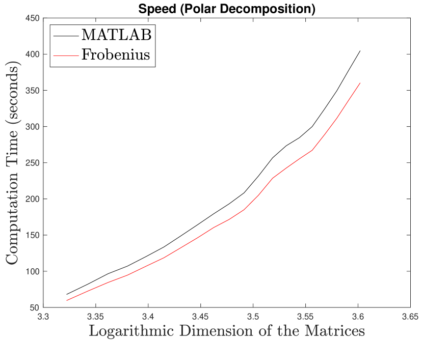
5.5. Polar decomposition

Another application of the matrix sign function is to polar decompose a given $X\in\mathbb{C}^{n\times n}$ into $X=QP$ with $Q\in\operatorname{U}_{n}(\mathbb{C})$ and $P\in\mathbb{C}^{n\times n}$ Hermitian positive semidefinite. This is based on the observation [31, 33, 39] that

\operatorname{sign}\biggl{(}\begin{bmatrix}0&X\\ X^{\scriptscriptstyle\mathsf{H}}&0\end{bmatrix}\biggr{)}=\begin{bmatrix}0&Q\\ Q^{\scriptscriptstyle\mathsf{H}}&0\end{bmatrix}.

Here the Newton iterations (26) take a slightly different form

X_{k+1}=\frac{1}{2}(X_{k}+X_{k}^{-{\scriptscriptstyle\mathsf{H}}}),\quad k=0,1,2,\dots,\quad X_{0}=X.

(27)

We generate random $Y,Z\in\mathbb{C}^{n\times n}$ with real and imaginary parts of its entries sampled uniformly from $[-1,1]$ . We then QR factorize $Y=UR$ and l set $P\coloneqq Z^{\scriptscriptstyle\mathsf{H}}Z$ and $X=UP$ . The value of $n$ runs from $2100$ to $4000$ .

Using the same stopping condition in Section 5.3 with a tolerance of $\varepsilon=10^{-3}$ and $k_{\max}=100$ maximum iterations, we compute a solution $\widehat{Q}$ with the Newton iterations (27), with $X_{k}^{-{\scriptscriptstyle\mathsf{H}}}$ computed by either Frobenius inversion or Matlab’s inversion. We then set $\widehat{P}=\widehat{Q}^{\scriptscriptstyle\mathsf{H}}X$ . Accuracy is measured by relative forward errors $\lVert Q-\widehat{Q}\rVert_{\max}/\lVert Q\rVert_{\max}$ and $\lVert P-\widehat{P}\rVert_{\max}/\lVert P\rVert_{\max}$ .

Figure 6 again shows that Frobenius inversion is faster than Matlab’s built-in inversion with near-identical accuracy. Indeed, at a scale of $10^{-3}$ for the vertical axis, the two graphs in the accuracy plot (right plot of Figure 6) are indistinguishable.

5.6. Hermitian positive definite matrix inversion

We repeat experiments in Section 5.1 on Hermitian positive definite matrices for our variant of Frobenius inversion (Algorithm 7) and Matlab’s built-in inversion based on Cholesky decomposition (Algorithm 8). For comparison, we also include Algorithms 4 and 5 that do not exploit Hermitian positive definiteness.

For our speed experiments, we generate a random Hermitian positive definite $X\coloneqq(A+iB)^{\scriptscriptstyle\mathsf{H}}(A+iB)+0.01I\in\mathbb{C}^{n\times n}$ with $A,B\in\mathbb{R}^{n\times n}$ sampled uniformly from $[-1,1]$ and $n$ from $3600$ to $6000$ . We plot the results in Figure 7, with two different scales for the horizontal axis.

For our accuracy experiments, we control the condition numbers of our matrices to reduce conditioning as a factor affecting accuracy. To generate a random Hermitian positive definite $X\in\mathbb{C}^{n\times n}$ with condition number $\kappa$ , first we generate a random unitary $Q\in\operatorname{U}_{n}(\mathbb{C})$ by QR factoring a random $Y\in\mathbb{C}^{n\times n}$ with real and imaginary parts of its entries sampled uniformly from $[-1,1]$ ; next we generate a random diagonal $\Lambda=\operatorname{diag}(\lambda_{1},\dots,\lambda_{n})\in\mathbb{R}^{n\times n}$ with $\lambda_{1}=\kappa$ , $\lambda_{n}=1$ , and $\lambda_{2},\dots,\lambda_{n-1}\in[1,\kappa]$ sampled uniform randomly; then we set $X\coloneqq Q\Lambda Q^{\scriptscriptstyle\mathsf{H}}/\lVert\Lambda\rVert_{\scriptscriptstyle\mathsf{F}}$ . So $\kappa(X)=\kappa$ . In the plots below, we set $\kappa=10$ and increase $n$ from $2$ through $4096$ .

Accuracy is measured by left and right relative residuals as defined in equation (23), with results plotted in Figure 8, which shows the left and right relative residuals computed by Algorithms 4, 5, 7, 8 plotted against matrix dimension $n$ . The important thing to note is the scale of the vertical axes — all four algorithms give essentially the same results up to machine precision.

6. Conclusion

We hope our effort here will rekindle interest in this beautiful algorithm. In future work, we plan to provide rounding error analysis for Frobenius inversion, discuss its relation with Strassen-style algorithms, and its advantage in solving linear systems with a large number of right-hand sides.

Acknowledgment

ZD acknowledges the support of DARPA HR00112190040 and NSF ECCF 2216912. LHL acknowledges the support of DARPA HR00112190040, NSF DMS 1854831, and a Vannevar Bush Faculty Fellowship ONR N000142312863. KY acknowledges the support of CAS Project for Young Scientists in Basic Research, Grant No. YSBR-008, National Key Research and Development Project No. 2020YFA0712300, and National Natural Science Foundation of China Grant No. 12288201.

References

[1] IEEE standard for floating-point arithmetic. In IEEE Std 754-2019 (Revision of IEEE 754-2008), pages 1–84. IEEE, New York, NY, 2019.
[2] H. Althaus and R. Leake. Inverse of a finite-field Vandermonde matrix (corresp.). IEEE Trans. Inform. Theory, 15(1):173–173, 1969.
[3] Z. Bai, J. Demmel, J. Dongarra, A. Petitet, H. Robinson, and K. Stanley. The spectral decomposition of nonsymmetric matrices on distributed memory parallel computers. SIAM J. Sci. Comput., 18(5):1446–1461, 1997.
[4] Z. Bai and J. W. Demmel. Design of a parallel nonsymmetric eigenroutine toolbox. University of Kentucky, Lexington, KY, 1992.
[5] A. N. Beavers, Jr. and E. D. Denman. A computational method for eigenvalues and eigenvectors of a matrix with real eigenvalues. Numer. Math., 21:389–396, 1973.
[6] A. S. Besicovitch. On the linear independence of fractional powers of integers. J. Lond. Math. Soc., 15:3–6, 1940.
[7] E. Bodewig. Matrix calculus. North-Holland, Amsterdam, enlarged edition, 1959.
[8] P. Bürgisser, M. Clausen, and M. A. Shokrollahi. Algebraic complexity theory, volume 315 of Grundlehren der mathematischen Wissenschaften. Springer-Verlag, Berlin, 1997.
[9] A. Caraiani and J. Newton. On the modularity of elliptic curves over imaginary quadratic fields. arXiv:2301.10509, 2023.
[10] S. Casacuberta and R. Kyng. Faster sparse matrix inversion and rank computation in finite fields. In 13th Innovations in Theoretical Computer Science Conference, ITCS 2022, pages 33:1–33:24. Dagstuhl Publishing, Germany, 2022.
[11] H. Cohen. A course in computational algebraic number theory, volume 138 of Graduate Texts in Mathematics. Springer-Verlag, Berlin, 1993.
[12] H. Cohen. Advanced topics in computational number theory, volume 193 of Graduate Texts in Mathematics. Springer-Verlag, New York, NY, 2000.
[13] H. Cramér. Mathematical Methods of Statistics, volume 9 of Princeton Mathematical Series. Princeton University Press, Princeton, NJ, 1946.
[14] Z. Dai and L.-H. Lim. Numerical stability and tensor nuclear norm. Numer. Math., to appear, 2023.
[15] A. Ditkowski, G. Fibich, and N. Gavish. Efficient solution of $Ax^{(k)}=b^{(k)}$ using $A^{-1}$ . J. Sci. Comput., 32(1):29–44, 2007.
[16] A. Druinsky and S. Toledo. How accurate is $\operatorname{inv}({A})*b$ ? arXiv:1201.6035, 2012.
[17] K. Dudeck. Solving complex systems using spreadsheets: A matrix decomposition approach. In Proceedings of the 2005 ASEE Annual Conference and Exposition: The Changing Landscape of Engineering and Technology Education in a Global World, pages 12875–12880. ASEE, Washington, DC, 2005.
[18] D. S. Dummit and R. M. Foote. Abstract algebra. John Wiley, Hoboken, NJ, third edition, 2004.
[19] S. Eberli, D. Cescato, and W. Fichtner. Divide-and-conquer matrix inversion for linear MMSE detection in SDR MIMO receivers. In Proceedings of the 26th IEEE Norchip Conference, pages 162–167. IEEE, New York, NY, 2008.
[20] W. Eberly. Processor-efficient parallel matrix inversion over abstract fields: Two extensions. In Proceedings of the 2nd International Symposium on Parallel Symbolic Computation, PASCO ’97, page 38–45. ACM, New York, NY, 1997.
[21] W. Eberly, M. Giesbrecht, P. Giorgi, A. Storjohann, and G. Villard. Faster inversion and other black box matrix computations using efficient block projections. In Proceedings of the 2007 International Symposium on Symbolic and Algebraic Computation, ISSAC ’07, page 143–150, New York, NY, USA, 2007. ACM, New York, NY.
[22] L. W. Ehrlich. Complex matrix inversion versus real. Comm. ACM, 13:561–562, 1970.
[23] M. El-Hawary. Further comments on “a note on the inversion of complex matrices”. IEEE Trans. Automat. Contr., 20(2):279–280, 1975.
[24] N. Freitas, B. V. Le Hung, and S. Siksek. Elliptic curves over real quadratic fields are modular. Invent. Math., 201(1):159–206, 2015.
[25] F. G. Frobenius. Gesammelte Abhandlungen. Bände I, II, III. Springer-Verlag, Berlin, 1968.
[26] M. Giesbrecht. Nearly optimal algorithms for canonical matrix forms. SIAM J. Comput., 24(5):948–969, 1995.
[27] P. E. Gill, G. H. Golub, W. Murray, and M. A. Saunders. Methods for modifying matrix factorizations. Math. Comp., 28:505–535, 1974.
[28] G. H. Golub. Matrix computation and the theory of moments. In Proceedings of the International Congress of Mathematicians, volume 2, pages 1440–1448. Birkhäuser, Basel, 1995.
[29] G. H. Golub and J. H. Wilkinson. Ill-conditioned eigensystems and the computation of the Jordan canonical form. SIAM Rev., 18(4):578–619, 1976.
[30] M. T. Heath, G. A. Geist, and J. B. Drake. Early experience with the Intel iPSC/860 at Oak Ridge National Laboratory. Int. J. High Perform. Comput. Appl., 5(2):10–26, 1991.
[31] N. J. Higham. Computing the polar decomposition—with applications. SIAM J. Sci. Statist. Comput., 7(4):1160–1174, 1986.
[32] N. J. Higham. Stability of a method for multiplying complex matrices with three real matrix multiplications. SIAM J. Matrix Anal. Appl., 13(3):681–687, 1992.
[33] N. J. Higham. The matrix sign decomposition and its relation to the polar decomposition. Linear Algebra Appl., 212/213:3–20, 1994.
[34] N. J. Higham. Accuracy and stability of numerical algorithms. SIAM, Philadelphia, PA, second edition, 2002.
[35] N. J. Higham. Functions of matrices. SIAM, Philadelphia, PA, 2008.
[36] J. Hoffstein, J. Pipher, and J. H. Silverman. An introduction to mathematical cryptography. Undergraduate Texts in Mathematics. Springer, New York, second edition, 2014.
[37] J. L. Howland. The sign matrix and the separation of matrix eigenvalues. Linear Algebra Appl., 49:221–232, 1983.
[38] A. A. Karatsuba. The complexity of computations. Trudy Mat. Inst. Steklov., 211:186–202, 1995.
[39] C. Kenney and A. J. Laub. On scaling Newton’s method for polar decomposition and the matrix sign function. SIAM J. Matrix Anal. Appl., 13(3):698–706, 1992.
[40] A. Klein and G. Mélard. Computation of the Fisher information matrix for time series models. J. Comput. Appl. Math., 64(1-2):57–68, 1995.
[41] D. E. Knuth. The art of computer programming. Vol. 2. Addison-Wesley, Reading, MA, third edition, 1998.
[42] C. Krattenthaler. A new matrix inverse. Proc. Amer. Math. Soc., 124(1):47–59, 1996.
[43] C. Lanczos. Applied analysis. Prentice-Hall, Englewood Cliffs, NJ, 1956.
[44] L.-H. Lim. Tensors in computations. Acta Numer., 30:555–764, 2021.
[45] C.-C. Lin and E. Zmijewski. A parallel algorithm for computing the eigenvalues of an unsymmetric matrix on an SIMD mesh of processors. University of California, Santa Barbara, CA, 1991.
[46] K. Lo. Several numerical methods for matrix inversion. Int. J. Electr. Eng. Educ., 15(2):131–141, 1978.
[47] J. H. Maindonald. Statistical computation. Series in Probability and Mathematical Statistics: Applied Probability and Statistics. John Wiley, New York, NY, 1984.
[48] P. McCullagh and J. A. Nelder. Generalized linear models. Monographs on Statistics and Applied Probability. Chapman & Hall, London, 1989.
[49] R. J. McEliece. Finite fields for computer scientists and engineers, volume 23 of International Series in Engineering and Computer Science. Kluwer, Boston, MA, 1987.
[50] A. J. Menezes, I. F. Blake, X. Gao, R. C. Mullin, S. A. Vanstone, and T. Yaghoobian. Applications of finite fields, volume 199 of International Series in Engineering and Computer Science. Kluwer, Boston, MA, 1993.
[51] M. Mignotte. Mathematics for computer algebra. Springer-Verlag, New York, NY, 1992.
[52] B. Mishra. Algorithmic algebra. Texts and Monographs in Computer Science. Springer-Verlag, New York, NY, 1993.
[53] P. Mukherjee and L. Satish. On the inverse of forward adjacency matrix. arXiv:1711.09216, 2017.
[54] I. Munro. Some results concerning efficient and optimal algorithms. In Proceedings of the Third Annual ACM Symposium on Theory of Computing, STOC ’71, page 40–44. ACM, New York, NY, 1971.
[55] M. L. Overton. Numerical computing with IEEE floating point arithmetic. SIAM, Philadelphia, PA, 2001.
[56] S. K. Panda. Inverses of bicyclic graphs. Electron. J. Linear Algebra, 32:217–231, 2017.
[57] S. Pavlíková. A note on inverses of labeled graphs. Australas. J. Combin., 67:222–234, 2017.
[58] C. R. Rao. Information and the accuracy attainable in the estimation of statistical parameters. Bull. Calcutta Math. Soc., 37:81–91, 1945.
[59] J. D. Roberts. Linear model reduction and solution of the algebraic Riccati equation by use of the sign function. Internat. J. Control, 32(4):677–687, 1980.
[60] S. Roman. Field theory, volume 158 of Graduate Texts in Mathematics. Springer, New York, NY, second edition, 2006.
[61] I. Schur. Gesammelte Abhandlungen. Band I, II, III. Springer-Verlag, Berlin, 1973.
[62] J. Schur. Über potenzreihen, die im innern des einheitskreises beschränkt sind. J. Reine Angew. Math., 148:122–145, 1918.
[63] W. W. Smith and J. Smith. Handbook of real-time fast Fourier transforms. IEEE, New York, NY, 1995.
[64] W. W. Smith, Jr. and S. Erdman. A note on the inversion of complex matrices. IEEE Trans. Automatic Contol, AC-19:64, 1974.
[65] D. R. Stinson and M. B. Paterson. Cryptography. Textbooks in Mathematics. CRC Press, Boca Raton, FL, fourth edition, 2019.
[66] C. Studer, S. Fateh, and D. Seethaler. ASIC implementation of soft-input soft-output MIMO detection using MMSE parallel interference cancellation. IEEE J. Solid-State Circuits, 46(7):1754–1765, 2011.
[67] L. Tornheim. Inversion of a complex matrix. Comm. ACM, 4:398, 1961.
[68] S. Winograd. On the number of multiplications necessary to compute certain functions. Comm. Pure Appl. Math., 23:165–179, 1970.
[69] D. Ye, Y. Yang, B. Mandal, and D. J. Klein. Graph invertibility and median eigenvalues. Linear Algebra Appl., 513:304–323, 2017.
[70] A. Zielinski. On inversion of complex matrices. Internat. J. Numer. Methods Engrg., 14(10):1563–1566, 1979.