Completion Delay of Random Linear Network Coding in Full-Duplex Relay Networks

We consider the two-hop full-duplex relay network depicted in Fig. 1, where a base station (BS) attempts to deliver $P$ packets to a set of $R$ receivers via a full-duplex relay station (RS) with a limited buffer size. The network transmission is considered to be time-slotted, that is, at every timeslot, the BS can deliver one packet to the RS, while the full-duplex RS can simultaneously fetch a coded packet from the BS and broadcast a coded packet to all receivers. The memoryless channel between the BS and the RS, together with the channel between the RS and every receiver $r$, are subject to independent random packet erasures with erasure probability $1-p_{0}$ and $1-p_{r}$, respectively. Every receiver is interested in recovering all $P$ original packets. Herein, the completion delay refers to the total number of packets transmitted by the BS before every receiver is able to recover all $P$ original packets. Notice that the definition of completion delay is the same as the one in [13][27], which takes the initial $P$ packets transmitted by the BS into account, so it is slightly different from the one in [13][6]. The packet number $P$ divided by the completion delay is set as a measurement of throughput in [27].

In practice, at every timeslot, even though the BS and the RS transmit simultaneously, the RS obtains what the BS transmits at the end of the timeslot. Thus, for the RS, the broadcast process is always one timeslot behind the reception process, i.e., what the RS broadcasts at timeslot $j$ has nothing to do with what it receives at timeslot $j$. Same as the consideration in [13], in this paper, we shall also ignore this constant timeslot lag at the RS and this assumption does not affect the analysis on the completion delay performance.

For the full-duplex relay network, Ref. [27] has proposed the FBPF scheduling scheme, in which if the RS buffer is not empty, the RS selects a packet that has been broadcast the fewest number of times from the unlimited buffer, and broadcasts the selected packets to the receivers. Since perfect RLNC is adopted in the design of the FBPF scheme, any $P$ different packets received by a receiver are assumed to be linearly independent.

Since the FBPF perfect RLNC scheme permits unlimited buffer at the RS for additional scheduling procedures, it is not a perfect RLNC scheme with the simplest setting at the RS. Thus, it does not reflect a fundamental performance guarantee provided by perfect RLNC in the full-duplex relay network, that is, there exist other perfect RLNC schemes with simpler settings at the RS and their completion delay performance is not as good as that of the FBPF scheme. On the other hand, the FBPF perfect RLNC scheme cannot yield the best performance gain in terms of completion delay as it does not involve NC at the RS.

In order to study the fundamental completion delay performance of perfect RLNC in the full-duplex relay network, we consider two basic perfect RLNC schemes, one without buffering at the RS and the other with buffering and recoding at the RS.

The first scheme, called perfect RLNC without buffer, does not require buffer and thus there is no recoding at the RS. The role of the RS is just to directly forward the received packets. At every timeslot, the BS delivers one coded packet, which is a random linear combination of $P$ original packets, to the RS. If the RS successfully receives the coded packet, then it will broadcast it to all receivers. Otherwise, the RS will not transmit anything. Notice that the full-duplex RS can simultaneously fetch the coded packet from the BS and broadcast it to all receivers. As perfect RLNC is considered, any $P$ coded packets generated by the BS are assumed linearly independent and sufficient to recover the $P$ original packets. As a result, once every receiver obtains $P$ packets, the transmission completes. Since this scheme does not involve any extra operation at the RS, it is the most straightforward and simplest application of perfect RLNC in the full-duplex relay network. As a result, it provides a fundamental performance guarantee for all perfect RLNC schemes designed for the full-duplex relay network in terms of completion delay.

The other scheme, called perfect RLNC with buffer, assumes buffer size $P$ and no coding constraints at the RS. At each timeslot, the BS transmits a coded packet to the RS, and if the RS receives the packet and its buffer is not full, then it stores the received packet in its buffer. Meanwhile, no matter whether the RS successfully receives the packet from the BS or not, it broadcasts a packet which is a random linear combination of all the packets stored in the buffer. Due to the causality at the RS to firstly buffer received packets and then broadcast a linear combination of buffered packets to receivers, the number of linearly independent packets obtained at a receiver is always no larger than the number of packets buffered at the RS. Once every receiver obtains $P$ linearly independent packets, the transmission completes. As perfect RLNC is considered, the $P$ original packets can be recovered from any $P$ coded packets generated by the BS. Moreover, there is no coding constraint at the RS in this scheme. As a result, as long as the RS stores $P$ coded packets transmitted from the BS, the $P$ original packets can be recovered from any $P$ randomly generated coded packets at the RS. This justifies why setting the buffer size to $P$ is sufficient, and actually, when the RS successfully stores $P$ coded packets transmitted from the BS in the buffer, there is no need for the BS to transmit new coded packets to the RS at all. To sum up, the scheme perfect RLNC with buffer attains the best completion delay performance among all perfect RLNC schemes in the full-duplex relay network.

In perfect RLNC without buffer, the completion delay at a single receiver $r$, denoted by $D_{0,r}$, is defined to be the number of packets the BS transmits till receiver $r$ is able to recover all $P$ original packets, and the completion delay for the system, denoted by $D_{0}$, is defined as

The completion delay $D_{0,r}$ at a single receiver $r$ follows the negative binomial distribution with the probability mass function $\mathrm{Pr}(D_{0,r}=P+d)=\binom{P+d-1}{P-1}(p_{0}p_{r})^{P}(1-p_{0}p_{r})^{d},d\geq 0$, so that the expectation of $D_{0,r}$ is equal to

For the special case that the channel from the RS to every receiver $r$ is perfect, i.e., $p_{r}=1$, the full-duplex relay network becomes essentially the same as a point-to-point transmission, so the system completion delay of both perfect RLNC schemes considered herein follows the negative binomial distribution with the expected value $\frac{P}{p_{0}}$. For the other special case $p_{0}=1$, the full-duplex relay network degenerates to the wireless broadcast with erasure probability $1-p_{r}$, so $\mathbb{E}[D_{0}]$ is given by $P+\sum\nolimits_{d\geq 0}(1-\prod\nolimits_{1\leq r\leq R}I_{p_{r}}(P,d+1))$, same as the one obtained in [6].

In perfect RLNC with buffer, the completion delay at receiver $r$ is denoted by $D_{P,r}$, where $P$ means the number of original packets generated by the source and to be recovered at every receiver. The system completion delay, denoted by $D_{P}$, is defined as

In order to characterize the expected completion delay $\mathbb{E}[D_{P,r}]$, we first recall the following combinatorial number

The Schroeder path (see, e.g., [34]) from $(0,0)$ to $(i,i)$ is a path with possible movement $(+1,0)$, $(0,+1)$, $(+1,+1)$ in every step transition and with $x\geq y$ for every point $(x,y)$ in the path. Then, $T_{i,j}$ represents the number of Schroeder paths from $(0,0)$ to $(i,i)$ with $i+j$ step transitions.

With $P$ increasing, the calculation of $\mathbb{E}[D_{P,r}]$ according to (5) becomes tedious because it involves the combinatorial number $T_{i,j}$, which can be extremely large. Stemming from (5), we next deduce an equivalent recurrence expression for $\mathbb{E}[D_{P,r}]$.

For $i\geq 0$, define

Thus, (5) can be rewritten as

Moreover, one can readily see

Based on (9) and (10), $\mathbb{E}[D_{P+1,r}]$ can be recursively computed for arbitrarily large $P$. It is also interesting to observe from Eq. (1), (5), (9) and (10) that the parameters $p_{0}$ and $p_{r}$ have the same impact on the expected completion delay at a single receiver $r$ for both perfect RLNC without buffer and perfect RLNC with buffer.

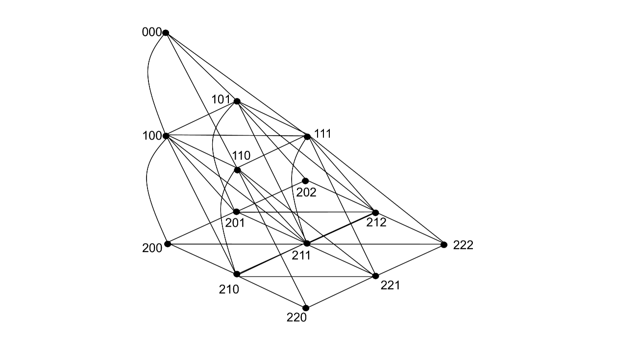
The transmission process of the perfect RLNC scheme with buffer for multiple receivers on the full-duplex relay network can be modeled as a Markov chain, denoted by $\mathcal{M}_{P,R}$, in the following way. Every state in $\mathcal{M}_{P,R}$ can be labeled by an $(R+1)$-tuple $\mathbf{s}=(s_{0},s_{1},s_{2},\ldots,s_{R})$, where $s_{0}$ represents the number of packets successfully received by the RS, and $s_{r}$ represents the number of packets successfully received by receiver $r$. Notice that $0\leq s_{r}\leq s_{0}\leq P$ for every receiver $r$. Thus, by conditioning on $s_{0}$, we can compute the number of states in the Markov chain $\mathcal{M}_{P,R}$ as $\sum_{s_{0}=0}^{P}(s_{0}+1)^{R}$ states. Except for the state $(P,P,\ldots,P)$, which is absorbing, all other $\sum_{s_{0}=0}^{P}(s_{0}+1)^{R}-1$ states are transient (assuming $p_{0},p_{1},\ldots,p_{R}\neq 0$). There is a $1$-step transition in the Markov chain once the BS broadcasts a new packet in a timeslot. An illustration of the $1$-step transition diagram for the case $R=P=2$ is given in Fig. 2. We next define the $1$-step transition probability from state $\mathbf{s}=(s_{0},s_{1},s_{2},\ldots,s_{R})$ to state $\mathbf{s}^{\prime}=(s_{0}^{\prime},s_{1}^{\prime},s_{2}^{\prime},\ldots,s_{R}^{\prime})$ for the Markov chain.

Let $\mathcal{R}$ denote the set of receivers who have not obtained $s_{0}$ packets at state $\mathbf{s}$ yet, that is, $\mathcal{R}=\{1\leq r\leq R:s_{r}<s_{0}\}$. In addition, denote by $\mathcal{R}^{\prime}$ the set of receivers who have obtained a new packet after the $1$-step transition from $\mathbf{s}$ to $\mathbf{s}^{\prime}$, that is, $\mathcal{R}^{\prime}=\{r\in\mathcal{R}:s_{r}^{\prime}=s_{r}+1\}$. The $1$-step transition probability from $\mathbf{s}$ to $\mathbf{s}^{\prime}$ can be formulated by the following $3$ different cases depending on the value of $s_{0}$ and $s_{0}^{\prime}$.

• •

  Case $1$: $s_{0}^{\prime}=s_{0}<P$. In this case $\mathcal{R}^{\prime}\subseteq\mathcal{R}$. We have

  $$p_{\mathbf{s},\mathbf{s}^{\prime}}=(1-p_{0})\left(\prod\nolimits_{r\in\mathcal{R^{\prime}}}p_{r}\right)\left(\prod\nolimits_{r\in\mathcal{R}\backslash\mathcal{R^{\prime}}}(1-p_{r})\right).$$

  (12)

• •

  Case $2$: $s_{0}^{\prime}=s_{0}=P$. In this case $\mathcal{R}^{\prime}\subseteq\mathcal{R}$. We have

  $$p_{\mathbf{s},\mathbf{s}^{\prime}}=\left(\prod\nolimits_{r\in\mathcal{R^{\prime}}}p_{r}\right)\left(\prod\nolimits_{r\in\mathcal{R}\backslash\mathcal{R^{\prime}}}(1-p_{r})\right).$$

  (13)

• •

  Case $3$: $s_{0}^{\prime}=s_{0}+1$. Notice that $\mathcal{R}^{\prime}$ is not necessarily contained in $\mathcal{R}$ in this case. We have

  $$p_{\mathbf{s},\mathbf{s}^{\prime}}=p_{0}\left(\prod\nolimits_{r\in\mathcal{R^{\prime}}}p_{r}\right)\left(\prod\nolimits_{r\notin\mathcal{R^{\prime}}}(1-p_{r})\right).$$

  (14)

Analogous to (6), the expected completion delay for the system can be expressed as

where $\mathbf{P}$ denotes the matrix of $1$-step transition probabilities among all transient states, with the first row/column indexed by the state $(0,\ldots,0)$.

Since the number of states in the Markov chain $\mathcal{M}_{P,R}$ increases exponentially with increasing $R$, it may not be convenient to compute $\mathbb{E}[D_{P}]$ based on (15). We next provide an alternative way to analyze $\mathbb{E}[D_{P}]$ by exploring its connection with $\mathbb{E}[\hat{D}_{P}]$, which is given by (3) and denotes the expected system completion delay for the special case $p_{0}=1$, or equivalently, the expected system completion delay in wireless broadcast. For this purpose, we first focus on a single receiver $r$ and compare $\mathbb{E}[D_{P,r}]$ with $\mathbb{E}[\hat{D}_{P,r}]=P/p_{r}$, which represents the expected completion delay at receiver $r$ for the special case $p_{0}=1$. For $1\leq j\leq P$, let $S_{j}$ and $T_{j,r}$ respectively denote the number of timeslots that the RS and receiver $r$ take to receive the $j^{th}$ packet. Thus, $S_{1}<\ldots<S_{P}$, $T_{1,r}<\ldots<T_{P,r}$, and $S_{j}\leq T_{j,r}$ for all $1\leq j\leq P$. By conditioning on the relation between $S_{P+1}$ and $T_{P,r}$, we can deduce the followings.

• •

  $S_{P+1}\leq T_{P,r}$, which means the RS has received the $(P+1)^{st}$ packet upon the reception of the $P^{th}$ packet by receiver $r$. In this case, it takes on average $\frac{1}{p_{r}}$ timeslots for receiver $r$ to further obtain the $(P+1)^{st}$ packet so that $\mathbb{E}[D_{P+1,r}]-\mathbb{E}[D_{P,r}]=\frac{1}{p_{r}}=\mathbb{E}[\hat{D}_{P+1,r}]-\mathbb{E}[\hat{D}_{P,r}]$;

• •

  $S_{P+1}>T_{P,r}$, which means upon the reception of the $(P+1)^{st}$ packet at the RS, receiver $r$ has only received fewer than $P$ packets. In this case, it takes on average $\frac{1}{p_{0}}$ additional timeslots for the RS to receive the $(P+1)^{st}$ packet, and $\frac{1}{p_{r}}-1$ timeslots for receiver $r$ to receive the $(P+1)^{st}$ packet. Thus, $\mathbb{E}[D_{P+1,r}]-\mathbb{E}[D_{P,r}]=\frac{1}{p_{0}}+\frac{1}{p_{r}}-1=\mathbb{E}[\hat{D}_{P+1,r}]-\mathbb{E}[\hat{D}_{P,r}]+\frac{1}{p_{0}}-1$.

In all, we have

Since $\mathbb{E}[D_{1,r}]=\frac{1}{p_{0}}+\frac{1}{p_{r}}-1$ and $\mathbb{E}[\hat{D}_{1,r}]=\frac{1}{p_{r}}$, we have

Moreover, due to (9), (16) and $\mathbb{E}[\hat{D}_{P+1,r}]-\mathbb{E}[\hat{D}_{P,r}]=\frac{1}{p_{r}}$, the following lemma can be obtained.

We next make a connection between $\mathbb{E}[D_{P}]$ and $\mathbb{E}[\hat{D}_{P}]$ similar to that between $\mathbb{E}[D_{P,r}]$ and $\mathbb{E}[\hat{D}_{P,r}]$ in (17). For $R$ independent geometrically distributed random variables $N_{1},\ldots,N_{R}$ (starting from $1$) with respective parameters $p_{1},\ldots,p_{R}$, define

$E_{\max}$ can be explicitly computed by the min-max identity (see, e.g., [35]). Based on $E_{\max}$,

For $P\geq 2$, the connection between $\mathbb{E}[D_{P}]$ and $\mathbb{E}[\hat{D}_{P}]$ can be analyzed by conditioning on the relation among $S_{P+1}$, $T_{P+1,r}$ and $T_{P,r}$, $1\leq r\leq R$. To ease the following presentation, we first elaborate the case of $R=2$, and then give a general conclusion for $R\geq 2$.

Let $\hat{T}_{j,r}$ denote the number of timeslots receiver $r$ takes to receive the $j^{th}$ packet in the special case $p_{0}=1$. Thus, (LABEL:eqn:recursive_expression_of_fullduplex1) implies

Let $\varepsilon_{P}$ denote the following identity

Eq. (23) in Theorem 6 extends (16) from the single receiver case to the case $R=2$. It implies an approximation, which can also serve as a lower bound, for $\mathbb{E}[D_{P}]$ based on $\mathbb{E}[\hat{D}_{P}]$. First, because $\mathrm{Pr}(S_{P+1}>T_{P,1}|S_{P+1}>T_{P,2})\geq\mathrm{Pr}(S_{P+1}>T_{P,1})$, we have

Since $\mathrm{Pr}(S_{P+1}>T_{P,1})$ and $\mathrm{Pr}(S_{P+1}>T_{P,2})$ can be explicitly computed based on Lemma 4 together with the recursive formula (10), we shall adopt $\mathrm{Pr}(S_{P+1}>T_{P,1})\mathrm{Pr}(S_{P+1}>T_{P,2})$ as an explicitly computable lower bound on $\mathrm{Pr}(S_{P+1}>\max\{T_{P,1},T_{P,2}\})$. Second, we shall omit $\varepsilon_{P+1}$ in the approximation whose performance will be justified below. For brevity, let $\tilde{D}_{P}$ denote

References

- [1] R. Su, Q. T. Sun and Z. Zhang, “On the delay of random linear network coding in full-duplex relay networks,” IEEE ISIT, 2021.
- [2] G. Liu, F. R. Yu, H. Ji, V. C. M. Leung and X. Li, “In-band full-duplex relaying: a survey, research issues and challenges,” IEEE Commun. Surv., vol. 17, no. 2, 2015.
- [3] T. Ho, M. Médard, R. Koetter, D. R. Karger, M. Effros, J. Shi and B. Leong, “A random linear network coding approach to multicast,” IEEE Trans. Inf. Theory, vol. 52, no. 10, 2006.
- [4] A. Eryilmaz, A. Ozdaglar, M. Medard and E. Ahmed, “On the delay and throughput gains of coding in unreliable networks,” IEEE Trans. Inf. Theory, vol. 54, no. 12, 2008.
- [5] E. Tsimbalo, A. Tassi and R. J. Piechocki, “Reliability of multicast under random linear network coding,” IEEE Trans. Commun., vol. 66, no. 6, 2018.
- [6] R. Su, Q. T. Sun and Z. Zhang, “Delay-complexity trade-off of random linear network coding in wireless broadcast,” IEEE Trans. Commun., vol. 68, no. 9, 2020.
- [7] I. Chatzigeorgious and A. Tassi, “Decoding delay performance of random linear network coding for broadcast,” IEEE Trans. Veh. Technol., vol. 66, no. 8, 2017.
- [8] B. T. Swapna, A. Eryilmaz, and N. B. Shroff, “Throughput-delay analysis of random linear network coding for wireless broadcasting,” IEEE Trans. Inf. Theory, vol. 59, no. 10, 2013.
- [9] D. E. Lucani, M. Medard and M. Stojanovic, “On coding for delay — network coding for time-division duplexing,” IEEE Trans. Inf. Theory, vol. 58, no. 4, 2012.
- [10] L. Wang, Y. Yang and W. Zhao, “Network coding-based multipath routing for energy efficiency in wireless sensor networks,” EURASIP J. WIREL. COMM., vol. 2012, 2012.
- [11] J. Huang, H. Gharavi, H. Yan and C. Xing, “Network coding in relay-based device-to-device communications,” IEEE Netw., vol. 31, no. 4, 2017.
- [12] S. Chieochan and E. Hossain, “Wireless fountain coding with IEEE 802.11E block ACK for media streaming in wireline-cum-Wifi networks: a performance study,” IEEE Trans. on Mob. Comput.,vol. 10, no. 10, 2011.
- [13] G. Giacaglia, X. Shi, M. Kim, D. E. Lucani and M. Médard, “Systematic network coding with the aid of a full-duplex relay,” IEEE ICC, 2013.
- [14] H. Khamfroush, P. Pahlevani, D. E. Lucani, M. Hundebøll and F. H. P. Fitzek, “On the coded packet relay network in the presence of neighbors: benefits of speaking in a crowded room,” IEEE ICC, 2014.
- [15] Y. Li, S. Blostein and W.-Y. Chan, “Systematic network coding for two-hop lossy transmissions,” EURASIP J. Adv. Signal Process, vol. 2015, 2015.
- [16] B. Maboudi, P. Pahlevani, “Security overhead of random linear network coding in multicast relay networks,” T. EMERG. TELECOMMUN. T., 2020.
- [17] C. Chen, S. J. Baek, and G. De Veciana, “Opportunistic scheduling of randomly coded multicast transmissions at half-duplex relay stations,” IEEE Trans. Inf. Theory, vol. 62, no. 10, 2016.
- [18] K. Loa, et al., “IMT-advanced relay standards [WiMAX/LTE update],” IEEE Commun. Mag., vol. 48, no. 8, 2010.
- [19] A. Damnjanovic, et al., “A survey on 3GPP heterogeneous networks,” IEEE Wireless Commun., vol. 18, no. 3, 2011.
- [20] P. Sadeghi, R. Shams and Danail Traskov, “An optimal adaptive network coding scheme for minimizing decoding delay in broadcast erasure channels,” EURASIP J. Wireless Commun. and Netw., vol. 2010, 2010.
- [21] S. Sorour and S. Valaee, “Completion delay minimization for instantly decodable network codes,” IEEE/ACM Trans. Netw., vol. 23, no. 5, 2015.
- [22] Z. Zhang, X. Chai, K. Long, A. V. Vasilakos and L. Hanzo, “Full duplex techniques for 5G networks: self-interference cancellation, protocol design, and relay selection,” IEEE Commun. Mag., vol. 53, no. 5, 2015.
- [23] Z. Zhang, K. Long, A. V. Vasilakos and L. Hanzo, “Full-duplex wireless communications: challenges, solutions, and future research directions,” Proc. IEEE, vol. 104, no. 7, 2016.
- [24] Y. Zhang, M. Xiao, S. Han, M. Skoglund and W. Meng, “On precoding and energy efficiency of full-duplex millimeter-wave relays,” IEEE Trans. Wirel. Commun., vol. 18, no. 3, 2019.
- [25] S. Han, Y. Zhang, W. Meng and H. Chen, “Self-interference-cancellation-based SLNR precoding design for full-duplex relay-assisted system,” IEEE Trans. Veh. Technol., vol. 67, no. 9, 2018.
- [26] H. Zhu, B. Smida and D. J. Love, “An efficient network-coded ARQ scheme for two-way wireless communication with full-duplex relaying,” IEEE Access, vol. 7, 2019.
- [27] C. Chen, Z. Meng, S. J. Baek, X. Yu, C. Li and R. Yin, “Low-complexity coded transmission without CSI for full-duplex relay networks,” IEEE GLOBECOM, 2020.
- [28] B. Shrader, A. Ephremides, “Queueing delay analysis for multicast with random linear coding,” IEEE Trans. Inf. Theory, vol. 58, no. 1, 2011.
- [29] H. Khamfroush, D.E. Lucani, and J. Barros, “Network coding for wireless coopertive networks: Simple rules, near-optimal delay,” in Proc. IEEE ICC Workshops, 2014.
- [30] D. E. Lucani, M. V. Pedersen, D. Ruano, C. W. Sørensen, F. H. P. Fitzek, J. Heide, O. Geil, V. Nguyen and M.Reisslein, “Fulcrum: flexible network coding for heterogeneous devices,” IEEE Access, vol. 6, 2018.
- [31] V. Nguyen, E. Tasdemir, G. T. Nguyen, D. E. Lucani, F. H. P. Fitzek, M.Reisslein, “DSEP Fulcrum: Dynamic sparsity and expansion packet for Fulcrum network coding,” IEEE Access, vol. 8, 2020.
- [32] A. Tassi, I. Chatzigeorgiou and D. E. Lucani, “Analysis and optimization of sparse random linear network coding for reliable multicast services,” IEEE Trans. Commun., vol. 64, no. 1, 2016.
- [33] J. Heide and D. Lucani, “Composite extension finite fields for low overhead network coding: telescopic codes,” IEEE ICC, 2015.
- [34] N. J. A. Sloane. The On-Line Encyclopedia of Integer Sequence. Accessed: 22nd, Jan. 2021[Online]. Available: https://oeis.org/A088617.
- [35] S. M. Ross, Introduction to Probability Models, Academic Press, 11th ed., 2014.
- [36] M. Nistor, D. E. Lucani, T. T. V. Vinhoza, R. A. Costa and J. Barros, “On the delay distribution of random linear network coding,” IEEE Journal on Selected Areas in Communications, vol. 29, no. 5, 2011.
- [37] J. Heide, M. V. Pedersen, F. H. P. Fitzek and M. Medard, “On code parameters and coding vector representation for practical RLNC,” IEEE ICC, 2011.
- [38] H. Tang, Q. T. Sun, Z. Li, X. Yang and K. Long, “Circular-shift linear network coding,” IEEE Trans. Inf. Theory, vol. 65, no. 1, 2019.
- [39] T. K. Petersen, Eulerian Numbers, Birkhuser Basel, 1st ed., 2015.