(eccv) Package eccv Warning: Package ‘hyperref’ is loaded with option ‘pagebackref’, which is *not* recommended for camera-ready version
11email: {nkadur,kmeibodi,soroush,hpirsiav}@ucdavis.edu
CompGS: Smaller and Faster Gaussian Splatting with Vector Quantization
Abstract
3D Gaussian Splatting (3DGS) is a new method for modeling and rendering 3D radiance fields that achieves much faster learning and rendering time compared to SOTA NeRF methods. However, it comes with a drawback in the much larger storage demand compared to NeRF methods since it needs to store the parameters for several 3D Gaussians. We notice that many Gaussians may share similar parameters, so we introduce a simple vector quantization method based on K-means to quantize the Gaussian parameters while optimizing them. Then, we store the small codebook along with the index of the code for each Gaussian. We compress the indices further by sorting them and using a method similar to run-length encoding. Moreover, we use a simple regularizer to encourage zero opacity (invisible Gaussians) to reduce the storage and rendering time by a large factor through reducing the number of Gaussians. We do extensive experiments on standard benchmarks as well as an existing 3D dataset that is an order of magnitude larger than the standard benchmarks used in this field. We show that our simple yet effective method can reduce the storage cost for 3DGS by to and rendering time by to with a very small drop in the quality of rendered images. Our code is available here: https://github.com/UCDvision/compact3d
1 Introduction
Recently, we have seen great progress in radiance field methods to reconstruct a 3D scene using multiple images captured from multiple viewpoints. NeRF [43] is probably the most well-known method that employs an implicit neural representation to learn the radiance field using a deep model. Although very successful, NeRF methods are very slow to train and render. Several methods have been proposed to solve this problem; however, they usually come with some cost in the quality of the rendered images.
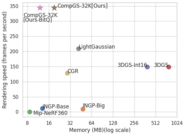
The Gaussian Splatting method (3DGS) [33] is a new paradigm in learning radiance fields. The idea is to model the scene using a set of Gaussians. Each Gaussian has several parameters including its position in 3D space, covariance matrix, opacity, color, and spherical harmonics of the color that need to be learned from multiple-view images. Thanks to the simplicity of projecting 3D Gaussians to the 2D image space and rasterizing them, 3DGS is significantly faster to both train and render compared to NeRF methods. This results in real-time rendering of the scenes on a single GPU (ref. Fig. 1). Additionally, unlike the implicit representations in NeRF, the 3D structure of the scene is explicitly stored in the parameter space of the Gaussians. This enables many operations including editing the 3D scene directly in the parameter space.
One of the main drawbacks of the 3DGS method compared to NeRF variants is that 3DGS needs at least an order of magnitude more parameters compared to NeRF. This increases the storage and communication requirements of the model and its memory at the inference time, which can be very limiting in many real-world applications involving smaller devices. For instance, the large memory consumption may be prohibitive in storing, communicating, and rendering several radiance field models on AR/VR headsets.
We are interested in compacting 3DGS representations without sacrificing their rendering speed to enable their usage in various applications including low-storage or low-memory devices and AR/VR headsets. Our main intuition is that several Gaussians may share some of their parameters (e.g. covariance matrix). Hence, we simply vector-quantize parameters while learning and store the codebook along with the index for each Gaussian. This can result in a huge reduction in the storage. Also, it can reduce the memory footprint at the rendering time since the index can act as a pointer to the correct code freeing the memory needed to replicate those parameters for all Gaussians.
To this end, we use simple K-means algorithm to vector quantize the parameters at the learning time. Inspired by various quantization-aware learning methods in deep learning [52], we use the quantized model in the forward pass while updating the non-quantized model in the backward pass. To reduce the computation overhead of running K-means, we update the centroids in each iteration, but update the assignments less frequently (e.g., once every 100 iterations) since it is costly. Moreover, since the Gaussians are a set of non-ordered elements, we compress the representation further by sorting the Gaussians based on one of the quantized indices and storing them using the Run-Length-Encoding (RLE) method. Furthermore, we employ a simple regularizer to promote zero opacity (essentially invisible Gaussians), resulting in a significant reduction in storage and rendering time by reducing the number of Gaussians. Our final model is to smaller and to faster during rendering compared to 3DGS.
2 Related Work
Novel-view synthesis methods: Early deep learning techniques for novel-view synthesis used CNNs to estimate blending weights or texture-space solutions [70, 17, 27, 62, 56]. However, the use of CNNs faced challenges with MVS-based geometry and caused temporal flickering. Volumetric representations began with Soft3D [50], and subsequent techniques used deep learning with volumetric ray-marching [29, 58]. Mildenhall et al. introduced Neural Radiance Fields (NeRFs) [43] to improve the quality of synthesized novel views, but the use of a large Multi-Layer Perceptron (MLP) as the backbone and dense sampling slowed down the process a lot. Successive methods sought to balance quality and speed, with Mip-NeRF360 achieving top image quality [4]. Recent advances prioritize faster training and rendering via spatial data structures, encodings, and MLP adjustments [18, 69, 28, 10, 19, 55, 67, 60, 45]. Notable methods, like InstantNGP [45], use hash grids and occupancy grids for accelerated computation with a smaller MLP, while Plenoxels [18] entirely forgo neural networks, relying on Spherical Harmonics for directional effects. Despite impressive results, challenges in representing empty space, limitations in image quality, and rendering speed persist in NeRF methods. In contrast, 3DGS [33] achieves superior quality and faster rendering without implicit learning [4]. However, the main drawback of 3DGS is its increased storage compared to NeRF methods which may limit its usage in many applications such as edge devices. We are able to keep the quality and fast rendering speed of 3DGS method while providing reduced model storage by applying a vector quantization scheme to Gaussian parameters.
Bit quantization: Reducing the number of bits to represent each parameter in a deep neural network is a commonly used method to quantize models [32, 26, 35] that result in smaller memory footprints. Representing weights in or -bit formats may not be crucial for a given task, and a lower-precision quantization can lead to memory and speed improvements. Dettmers et al. [14] show 8-bit quantization is sufficient for large language models. In the extreme case, weights of neural networks can be quantized using binary values. XNOR [53] examines this extreme case by quantization-aware training of a full-precision network that is robust to quantization transformations.
Vector quantization: Vector quantization (VQ) [23, 20, 15, 22] is a lossy compression technique that converts a large set of vectors into a smaller codebook and represents each vector by one of the codes in the codebook. As a result, one needs to store only the code assignments and the codebook instead of storing all vectors. VQ is used in many applications including image compression [12], video and audio codec [38, 42], compressing deep networks [11, 22], and generative models [63, 24, 54]. We apply a similar method to compressing 3DGS models.
Deep model compression. Model compression tries to reduce the storage size without changing the accuracy of original models. Model compression techniques can be divided to 1) model pruning [25, 26, 64, 66] that aims to remove redundant layers of neural networks; 2) weight quantization [48, 32, 35], and 3) knowledge distillation [3, 30, 9, 51, 2], in which a compact student model is trained to mimic the original teacher model. Some works have applied these techniques to volumetric radiance fields [13, 40, 69]. For instance, TensoRF [8] decompose volumetric representations via low-rank approximation.
Compression for 3D scene representation methods. Since NeRF relies on dense sampling of color values and opacity, the computational costs are significant. To increase efficiency, methods adopt different data structures such as trees [65, 69], point clouds [68, 49], and grids [8, 18, 45, 57, 59, 60]. With grid structures training iterations can be completed in a matter of minutes. However, dense 3D grid structures may require substantial amounts of memory. Several methods have worked on reducing the size of such volumetric grids [61, 8, 60, 45]. Instant-NGP [45] uses hash-based multi-resolution grids. VQAD [60] replaces the hash function with codebooks and vector quantization.
Another line of work decomposes 3D grids into lower dimensional components, such as planes and vectors, to reduce the memory requirements [8, 61, 31]. Despite reducing the time and space complexity of the 3D scenes, their sizes are still larger than MLP-based methods. VQRF [39] compresses volumetric grid-based radiance fields by adopting the VQ strategy to encode color features into a compact codebook.
While we also employ vector quantization, we differ from the above approaches in the method employed for novel view synthesis. Unlike the NeRF based approaches described above, we aim to compress 3DGS which uses a collection of 3D Gaussians to represent the 3D scene and does not contain grid like structures or neural networks. We also achieve a significant amount of compression by regularizing and pruning the Gaussians based on their opacity.
Concurrent works: Some very recent works developed concurrently to ours [46, 16, 36, 44, 21] also propose vector quantization and pruning based methods to compress 3D Gaussian splat models. LightGaussian [16] uses importance based Gaussian pruning and distillation and vector quantization of spherical harmonics parameters. Similarly, CGR [36] masks Gaussians based on their volume and transparency to reduce the number of Gaussians and uses residual vector quantization for scale and rotation parameters. In CGS [46], highly sensitive parameters are left non-quantized while the less sensitive ones are vector quantized.
3 Method
Here, we briefly describe the 3DGS [33] method for learning and rendering 3D scenes and explain our vector quantization approach for compressing it.
Overview of 3DGS: 3DGS models a scene using a collection of 3D Gaussians. A 3D Gaussian is parameterized by its position and covariance matrices in the 3D space. where is the position vector, is the position, and is the 3D covariance matrix of the Gaussian. Since the covariance matrix needs to be positive definite, it is factored into its scale () and rotation () matrices as for easier optimization. In addition, each Gaussian has an opacity parameter . Since the color of the Gaussians may depend on the viewing angle, the color of each Gaussian is modeled by a Spherical Harmonics (SH) of order 3 in addition to a DC component.
Given a view-point, the collection of 3D Gaussians is efficiently rendered in a differentiable manner to get a 2D image by -blending of anisotropic splats, sorting, and using a tile-based rasterizer. Color of a pixel is given by
where is the color of the Gaussian and is
the product of the value of the Gaussian at that point and its learned opacity . At the training time, 3DGS minimizes the loss between the groundtruth and rendered images in the pixel space.
The loss is loss plus an SSIM loss in the pixel space. 3DGS initializes the optimization by a point cloud achieved by a standard SfM method and iteratively prunes the ones with small opacity and adds new ones when the gradient is large. 3DGS paper shows that it is extremely fast to train and is capable of real-time rendering while matching or outperforming SOTA NeRF methods in terms of rendered image quality.
Compression of 3DGS:
We compress the parameters of 3DGS using vector quantization aware training and reduce the number of Gaussians by regularizing the opacity parameter.
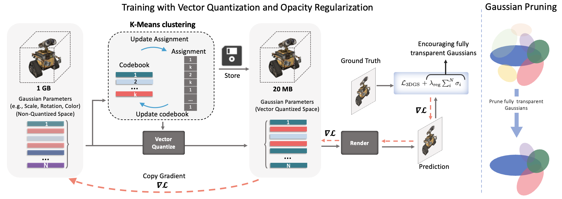
Vector quantization: 3DGS requires a few million Gaussians to model a typical scene. With parameters per Gaussian, the storage size of the trained model is an order of magnitude larger than most NeRF approaches (e.g., Mip-NeRF360 [4]). This makes it inefficient for some applications including edge devices. We are interested in reducing the number of parameters. Our main intuition is that many Gaussians may have similar parameter values (e.g., covariance). Hence, we use simple vector quantization using K-means algorithm to compress the parameters. Fig. 2 provides an overview of our approach.
Consider a 3DGS model with Gaussians, each with a dimensional parameter vector. We run K-means algorithm to cluster the vectors into clusters. Then, one can store the model using vectors of size and integer indices (one for each Gaussian). Since , this method can result in a large compression ratios. In a typical scene, is a few millions while is a few thousands.
However, clustering the model parameters after training results in performance degradation, hence, we perform quantization aware training to ensure that the parameters are amenable to quantization. In learning 3DGS, we store the non-quantized parameters. In the forward pass of learning 3DGS, we quantize the parameters and replace them with the quantized version (centroids) to do the rendering and calculate the loss. Then, we do the backward pass to get the gradients for the quantized parameters and copy the gradients to the non-quantized parameters to update them. We use straight-through estimator proposed in STE [7]. After learning, we discard the non-quantized parameters and keep only the codebook and indices of the codes for Gaussians.
Since the number of Gaussians is typically in millions, cost of performing K-means at every iteration of training can be prohibitively high. K-means has two steps: updating centroids given assignments, and updating assignments given centroids. We note that the latter is more expensive while the former is a simple averaging. Hence, we update the centroids after each iteration and update the assignments once every iterations. We observe that the modified approach works well even for values of as high as . This is crucial in limiting the training time of the method.
Performing a single K-means for the whole dimensional parameters requires a huge codebook since the different parameters of the Gaussian are not necessarily correlated. Hence, we group similar types of parameters, e.g., all rotation matrices, together and cluster them independently to learn a separate codebook for each. This requires storing multiple indices for each Gaussian. In our main method, we quantize DC component of color, spherical harmonics, scale, and rotation parameters separately, resulting in codebooks. We do not quantize opacity parameter since it is a single scalar and do not quantize the position of the Gaussians since sharing them results in overlapping Gaussians.
Since the indices are integer values, we use fewer number of bits compared to the original parameters to store each. Moreover, 3DGS models the scene as a set of order-less Gaussians. Hence, we sort the Gaussians based on one of the indices, e.g., rotation, so that Gaussians using the same code appear together in the list. Then, for that index, instead of storing integers, we store how many times each code appears in the list, reducong the storage from integers to integers. This is similar to run-length-encoding for data compression.
Opacity Regularization: Some parameters like position of the Gaussians cannot be quantized easily, so as shown in Table 7 after quantization, they dominate the memory(more than 80% of memory). This means quantization cannot improve the compression any further. One way to compress 3DGS more is to reduce the number of Gaussians. Interestingly, this reduction comes with a bi-product that is increase in inference speed. We know that very small values of opacity () correspond to transparent or nearly invisible Gaussians. Hence, inspired by training sparse models, we add norm of the opacity to the loss as a regularizer to encourage zero values for opacity. Therefore, the final loss becomes: , where is the original loss of 3DGS with or without quantization and controls the sparsity of opacity. Finally, similar to the original 3DGS, we remove the Guassians with opacity smaller than a threshold, resulting in significant reduction in storage and inference time.
4 Experiments
Implementation details: For all our experiments, we use the publicly available
official code repository [1] of 3DGS [33] provided by its authors.
There are no changes in the hyperparameters used for training compared to 3DGS. The Gaussian
parameters are trained without any vector quantization till iterations and K-means quantization is
used for the remaining iterations. A standard K-means iteration involves
distance calculation between all elements (Gaussian parameters) and all cluster centers followed by assignment
to the closest center. The centers are then updated using new cluster assignments and the loop is repeated.
We use just such K-means iteration in our experiments once every iterations
till iteration and keep the assignments constant thereafter till the last iteration, .
The K-means cluster centers are
updated using the non-quantized Gaussian parameters after each iteration of training.
The covariance (scale and rotation) and color
(DC and harmonics) components of each Gaussian is vector quantized while position (mean) and opacity parameters are not quantized. Additional results with different parameters being quantized
are provided in Table 9. Unless mentioned differently, we use a codebook of size for the color
and (CompGS ) for the covariance parameters. The scale parameters of covariance are quantized before applying
the exponential activation on them. Similarly, quaternion based rotation parameters are quantized before
normalization. For opacity regularization, we use from iterations to
along with opacity based pruning every iterations and remove regularization thereafter.
All experiments were run on a single RTX- GPU.
| Mip-NeRF360 | Tanks&Temples | |||||||||||
| Method | SSIM↑ | PSNR↑ | LPIPS↓ | FPS | Mem (MB) | Train Time(m) | SSIM↑ | PSNR↑ | LPIPS↓ | FPS | Mem (MB) | Train Time(m) |
| Plenoxels† [18] | 0.626 | 23.08 | 0.463 | 6.79 | 2,100 | 25.5 | 0.719 | 21.08 | 0.379 | 13.0 | 2300 | 25.5 |
| INGP-Base† [45] | 0.671 | 25.30 | 0.371 | 11.7 | 13 | 5.37 | 0.723 | 21.72 | 0.330 | 17.1 | 13 | 5.26 |
| INGP-Big† [45] | 0.699 | 25.59 | 0.331 | 9.43 | 48 | 7.30 | 0.745 | 21.92 | 0.305 | 14.4 | 48 | 6.59 |
| M-NeRF360† [4] | 0.792 | 27.69 | 0.237 | 0.06 | 8.6 | 48h | 0.759 | 22.22 | 0.257 | 0.14 | 8.6 | 48h |
| 3DGS † [33] | 0.815 | 27.21 | 0.214 | 134 | 734 | 41.3 | 0.841 | 23.14 | 0.183 | 154 | 411 | 26.5 |
| 3DGS ∗ [33] | 0.813 | 27.42 | 0.217 | 21.6 | 0.844 | 23.68 | 0.178 | 12.2 | ||||
| LigthGaussian [16] | 0.805 | 27.28 | 0.243 | 209 | 42 | - | 0.817 | 23.11 | 0.231 | 209 | 22 | - |
| CGR [37] | 0.797 | 27.03 | 0.247 | 128 | 29.1 | - | 0.831 | 23.32 | 0.202 | 185 | 20.9 | - |
| CGS [47] | 0.801 | 26.98 | 0.238 | - | 28.8 | - | 0.832 | 23.32 | 0.194 | - | 17.28 | - |
| CompGS 16K | 0.804 | 27.03 | 0.243 | 22.8 | 0.836 | 23.39 | 0.200 | 15.6 | ||||
| CompGS 32K | 0.806 | 27.12 | 0.240 | 344 | 19 | 29.4 | 0.838 | 23.44 | 0.198 | 475 | 13 | 20.6 |
| CompGS 32K BitQ | 0.797 | 26.97 | 0.245 | 29.4 | 0.832 | 23.35 | 0.202 | 20.6 | ||||
Datasets: We primarily show results on three challenging real world datasets -
Tanks&Temples[34], Deep Blending [27] and Mip-NeRF360 [4]
containing two, two and nine scenes respectively.
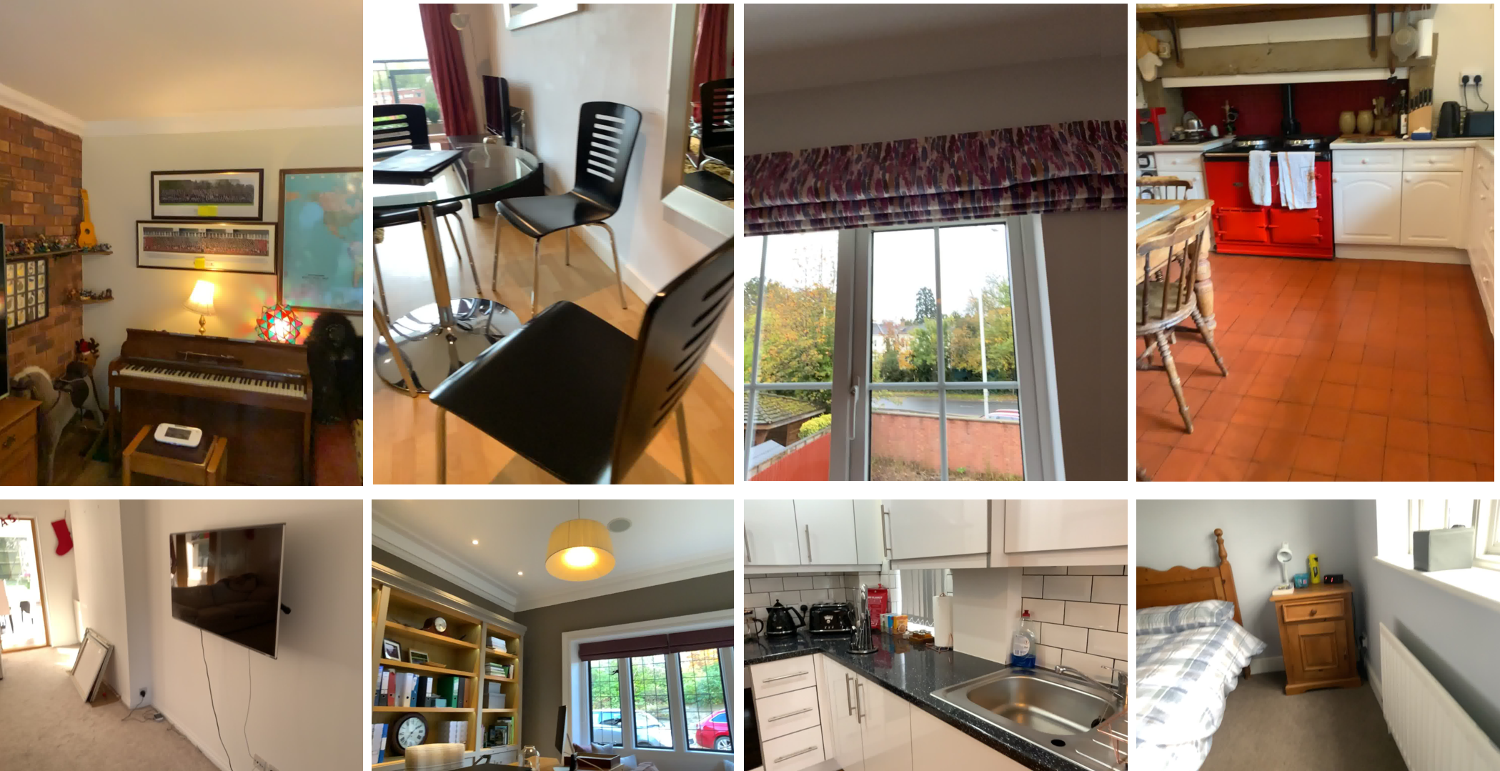
Also, we provide results on a subset of the recently released DL3DV-10K dataset [41] which contains 140 scenes. DL3DV-10K [41] is an annotated dataset with real-world scene-level videos. Out of these, scenes have been used to create a novel-view synthesis (NVS) benchmark, making it an order of magnitude larger than the typical NVS benchmarks. We use this NVS benchmark in our experiments. Additionally, we provide results on a subset of the large scale ARKit [6]
dataset, called ARKit-200, which contains scenes. Details of this dataset is presented in the Appendix.
Baselines: As we propose a method (termed CompGS)
for compacting 3DGS, we focus our comparisons with
3DGS and different baseline methods for compressing it. We consider bit quantization (denoted as Int-16/8/4 in
results) and 3DGS without the harmonic components for color (denoted as 3DGS-No-SH) as alternative parameter compression
methods. Bit-quantization is performed using the standard Absmax quantization [14] technique.
Similarly, we consider several alternative approaches to reduce the number of Gaussians.
Densification process in 3DGS increases the Gaussian count and is controlled by the gradient threshold (termed grad thresh) parameter and the
frequency (freq) and iterations (iters) until densification is performed. The opacity threshold (min opacity) controls the pruning of transparent
Gaussians. We modify these parameters in 3DGS to compress the model with as little drop in performance as possible.
Additionally, Table 1 shows comparison with state-of-the-art NeRF
approaches [4, 18, 45].
Mip-NeRF360 [4] achieves high performance comparable to 3DGS while
Plenoxels [18] and InstantNGP[45] have high frame-rate for
rendering and very low training time. InstantNGP and Mip-NeRF360 are also comparable in model size to our
compressed model.
Evaluation: For a fair comparison, we use the same train-test split as
Mip-NeRF360 [4] and 3DGS [33] and directly report the metrics for other
methods from 3DGS [33]. We also report our reproduced metrics for 3DGS since we observe slightly better results compared to the ones in [33]. We report the standard evaluation
metrics of SSIM, PSNR and LPIPS along with memory or compression ratio, rendering FPS and training time. The common practice is to report the average of PSNR across a set of images and scenes.
However, this metric may be dominated by very accurate reconstructions (smaller errors) since it is based on the geometric average of the errors due to the log operation in PSNR calculation. Hence, for the larger ARKit dataset, we also report PSNR-AM for which we average the error across all images and scenes before calculating the PSNR. In comparing model sizes, we normalize all methods by dividing them by the size of our method to obtain compression ratio.
| Mip-NeRF360 | Tanks&Temples | Deep Blending | ||||||||
| Method | SSIM | PSNR | LPIPS | SSIM | PSNR | LPIPS | SSIM | PSNR | LPIPS | Mem |
| 3DGS | 0.813 | 27.42 | 0.217 | 0.844 | 23.68 | 0.178 | 0.899 | 29.49 | 0.246 | 20.0 |
| 3DGS-No-SH | 0.802 | 26.80 | 0.229 | 0.833 | 23.16 | 0.190 | 0.900 | 29.50 | 0.247 | 4.8 |
| Post-train K-means 4K | 0.768 | 25.46 | 0.266 | 0.803 | 22.12 | 0.226 | 0.887 | 28.61 | 0.268 | 1.7 |
| K-means 4K Only-SH | 0.811 | 27.25 | 0.223 | 0.842 | 23.57 | 0.183 | 0.902 | 29.60 | 0.246 | 4.8 |
| K-means 4K | 0.804 | 26.97 | 0.234 | 0.836 | 23.31 | 0.194 | 0.904 | 29.76 | 0.248 | 1.7 |
| K-means 32K | 0.808 | 27.16 | 0.228 | 0.840 | 23.47 | 0.188 | 0.903 | 29.75 | 0.247 | 1.8 |
| Int16 | 0.804 | 27.25 | 0.223 | 0.836 | 23.56 | 0.185 | 0.900 | 29.49 | 0.247 | 10.0 |
| Int8 no-pos | 0.812 | 27.38 | 0.219 | 0.843 | 23.67 | 0.180 | 0.900 | 29.47 | 0.247 | 5.8 |
| Int8 | 0.357 | 14.41 | 0.629 | 0.386 | 12.37 | 0.625 | 0.709 | 21.58 | 0.457 | 5.0 |
| Int4 no-pos | 0.489 | 17.42 | 0.525 | 0.488 | 12.94 | 0.575 | 0.746 | 19.90 | 0.446 | 3.4 |
| 3DGS-No-SH Int16 | 0.789 | 26.59 | 0.237 | 0.826 | 23.04 | 0.198 | 0.900 | 29.50 | 0.248 | 2.4 |
| K-means 4K, Int16 | 0.796 | 26.83 | 0.239 | 0.830 | 23.21 | 0.199 | 0.904 | 29.76 | 0.248 | 1.0 |
Results:
Comparison of our results with SOTA novel view synthesis approaches is shown in Table 1.
Our vector quantized method has a comparable performance to the non-quantized 3DGS with a small drop on MipNerf-360 and
TandT datasets and a small improvement on the DB dataset. We additionally report results with post-training bit quantization of our model (CompGS BitQ) where the position and opacity parameters are quantized to bits and bits respectively.
The model memory footprint drastically reduces for CompGS compared to 3DGS , making it comparable to NeRF approaches. Our
models are and smaller than 3DGS models on MipNerf-360 and TandT datasets respectively.
This reduces a big disadvantage of 3DGS models and
makes them more practical. The compression achieved by CompGS is impressive considering that more than
two-thirds of its memory is due to the non-quantized position and opacity parameters (refer table 7).
Additionally CompGS maintains the other advantages of 3DGS such as low inference memory usage and training time.
while also increasing its already impressive rendering FPS by to .
A limitation of CompGS compared to 3DGS is the overhead in compute and training
time introduced by the K-means clustering algorithm. This is compensated in part by the reduced compute and time due
to the decrease in Gaussian count. CompGS 16K variant requires marginally more time than 3DGS while CompGS 32K needs
to more training time.
However, this is still orders of magnitude smaller than the high-quality NeRF based approaches like MipNerf-360.
Per-scene evaluation metrics are in Appendix. Note that there are large differences in reproduced results for 3DGS across various works in the literature. We observe a median standard deviation of dB for PSNR when the experiment is repeated times with several scenes having differences more than dB across runs (refer Appendix). One must be careful when analyzing as these variations are often comparable to differences in performance between methods.
We decouple our compression method into parameter and Gaussian count compression components and perform ablations on each of them.
Comparison of parameter compression methods: In Table 2, we compare the proposed vector quantization based compression against other baseline approaches for compressing 3DGS. Since the spherical harmonic components used for modeling color make up nearly three-fourths of all the parameters of each Gaussian, a trivial compression baseline is to use a variant of 3DGS with only the DC component for color and no harmonics. This baseline (3DGS-No-SH ) achieves a high compression with just of the original model size but has a drop in performance. Our K-Means approach outperforms 3DGS-No-SH while using less than half its memory. We also consider a variant of CompGS with a single codebook for both SH and DC parameters (termed SH+DC) with a larger codebook of size of . This has a marginal decrease in both memory and performance compared to default CompGS suggesting that correlated parameters can be combined to reduce the number of indices to be stored.
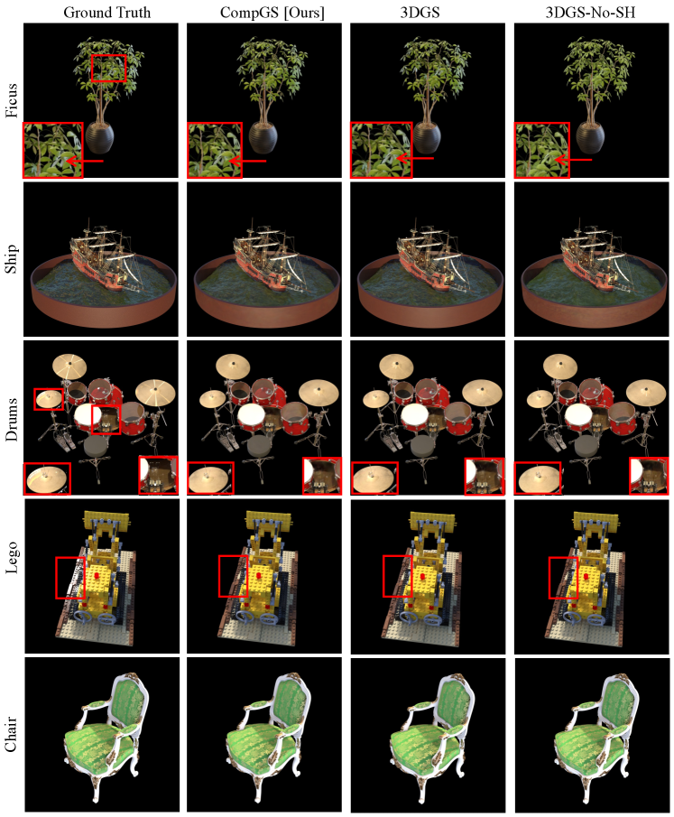
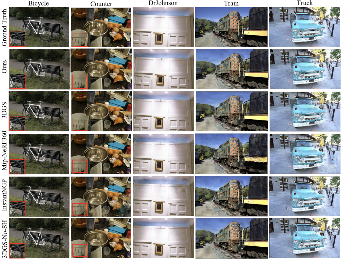
Fig. 3 shows qualitative comparison of CompGS across multiple datasets with both SOTA approaches and compression methods for 3DGS . Both CompGS and 3DGS-No-SH are visually similar to 3DGS, preserving finer details such as the spokes of the bike and bars of dish-rack. Among NeRF approaches, Mip-NeRF360 is closest in terms of quality to 3DGS while InstantNGP trades-off quality for inference and training speed.
| Mip-NeRF360 | Tanks&Temples | Deep Blending | ||||||||||
| Method | SSIM | PSNR | LPIPS | #Gauss | SSIM | PSNR | LPIPS | #Gauss | SSIM | PSNR | LPIPS | #Gauss |
| 3DGS | 0.813 | 27.42 | 0.217 | 0.844 | 23.68 | 0.178 | 0.899 | 29.49 | 0.246 | |||
| Min Opacity | 0.802 | 27.12 | 0.244 | 1.46M | 0.833 | 23.44 | 0.204 | 780K | 0.902 | 29.50 | 0.255 | 1.01M |
| Densify Freq | 0.794 | 26.98 | 0.255 | 1.07M | 0.832 | 23.36 | 0.206 | 709K | 0.902 | 29.76 | 0.258 | 844K |
| Densify Iters | 0.780 | 27.02 | 0.267 | 1.12M | 0.835 | 23.55 | 0.194 | 810K | 0.896 | 29.42 | 0.264 | 795K |
| Grad Thresh | 0.769 | 26.57 | 0.292 | 809K | 0.825 | 23.31 | 0.217 | 578K | 0.900 | 29.49 | 0.260 | 1.01M |
| Opacity Reg | 0.813 | 27.42 | 0.227 | 0.844 | 23.71 | 0.188 | 0.905 | 29.73 | 0.249 | |||
All the above approaches are trained using -bit precision for all Gaussian parameters. Post-training bit
quantization of 3DGS to -bits reduces the memory by half with very little drop in performance.
However, reducing the precision to -bits results in a huge degradation of the model.
This drop is due to the quantization of the position parameters of the Gaussians. Excluding them from
quantization (denoted as Int8 no-pos) results in a model comparable to the -bit variant. However, further
reduction to -bits degrades the model even when the position parameters are not quantized. Note that
bit quantization approaches offer significantly lower compression compared to CompGS and they are a subset
of the possible solutions for our vector quantization method. Similar to 3DGS, CompGS has a small drop in performance when -bit quantization is used.
| Method | SSIM | PSNR | PSNR-AM | LPIPS | Mem |
| 3DGS | 0.909 | 25.76 | 20.73 | 0.226 | 20.0 |
| 3DGS-No-SH | 0.905 | 25.31 | 20.11 | 0.234 | 4.8 |
| CompGS | 0.909 | 25.70 | 20.73 | 0.229 | 1.7 |
![[Uncaptioned image]](https://cdn.awesomepapers.org/papers/14456b82-abee-4c4f-b8d9-61f15c7a8564/ARKit.png)
| DL3DV-140 | ||||||
| Method | SSIM↑ | PSNR↑ | PSNR-AM↑ | LPIPS↓ | FPS | Mem(MB) |
| 3DGS * | 0.905 | 29.06 | 27.37 | 0.134 | 282 | 291 |
| CompGS 32K | 0.895 | 28.42 | 26.97 | 0.149 | 566 | 10 |
Comparison of Gaussian count compression methods: In Table 3, we compare the proposed opacity regularization
method for reducing the Gaussian count with baselines. In these baselines, we modify the 3DGS parameters to decrease densification and increase pruning
and thus reduce the number of Gaussians. We report the best metrics for each baseline here (refer Appendix for ablation). Our opacity regularization results in
to reduction in Gaussian count with nearly identical performance as the larger models. Similar level of compression
is achieved only by the gradient threshold baseline that reduces densification.
However, it results in a large drop in performance.
| Non | Quant | |
| Quant | ||
| Num Params | 4 | 55 |
| Mem (16bit) | 68% | 32% |
| Mem (32bit) | 81% | 19% |
| k-Means Quantization | |
| Index | Codebook |
| 99% | 1% |
| 98% | 2% |
| SSIM | PSNR | LPIPS | #Gauss | |
| 1.21M | ||||
| 0.806 | 27.12 | 0.240 | 845K | |
| 0.801 | 26.98 | 0.253 | 536K | |
| 0.794 | 26.83 | 0.266 |
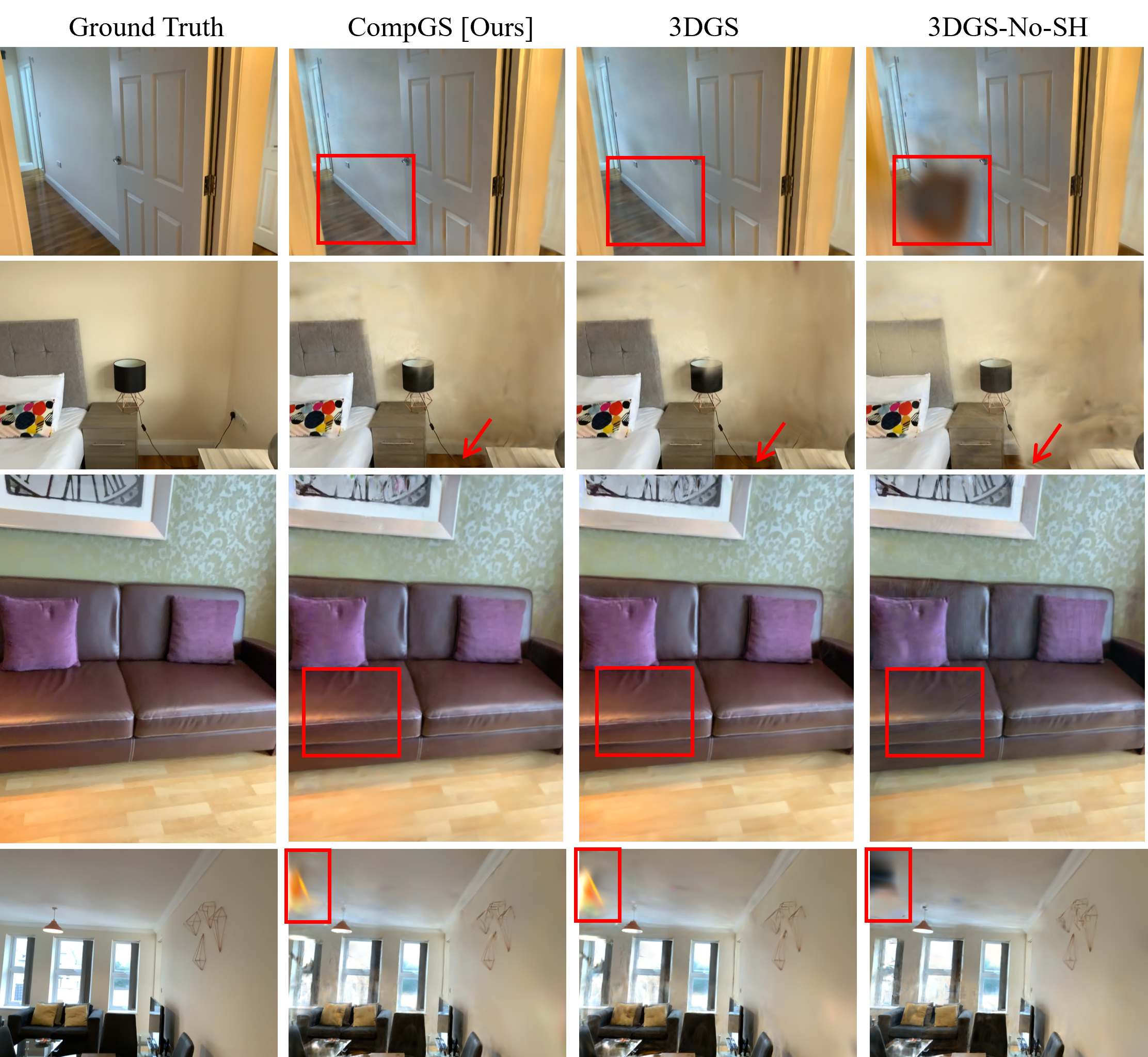
Results on ARKit-200 and DL3DV datasets: Table 4 shows the quantitative and qualitative results on our large-scale ARKit-200 benchmark. Our compressed model achieves nearly the same performance as 3DGS with ten times smaller memory. Unlike CompGS , the 3DGS-No-SH method suffers a significant drop in quality. We also report PSNR-AM as the PSNR calculated using arithmetic mean of MSE over all the scenes in the dataset to prevent the domination of high-PSNR scenes. Similarly, Table 5 shows the performance of CompGS with both KMeans quantization and opacity regularization. CompGS achieves nearly compression compared to 3DGS with a small drop in performance.
4.1 Ablations
We analyze our design choices and the effect of various hyperparameters on reconstruction performance and model size.
Memory break-down of CompGS: In Table 7, we show the
contribution of various components to the final memory usage of CompGS . Out of parameters of each
Gaussian, we quantize parameters of color and covariance while the position and opacity
parameters are used as is. However, the bulk of the stored memory ( and for 16- and 32-bits)
is due to the non-quantized parameters. For the quantized parameters, nearly all the memory is used to
store the cluster assignment indices with less than used for the codebook.
| Iters | Freq | #Codes | SSIM | PSNR | Time |
| 1 | 100 | 8K | 0.802 | 26.94 | 19.3 |
| 3 | 100 | 8K | 0.802 | 26.94 | 20.9 |
| 5 | 100 | 8K | 0.802 | 26.95 | 22.5 |
| 10 | 100 | 8K | 0.802 | 26.95 | 26.5 |
| 5 | 50 | 8K | 0.803 | 27.00 | 28.7 |
| 5 | 200 | 8K | 0.799 | 26.76 | 19.4 |
| 5 | 500 | 8K | 0.783 | 26.15 | |
| 5 | 100 | 4K | 0.800 | 26.84 | 19.6 |
| 5 | 100 | 16K | 0.804 | 27.05 | 28.9 |
| 5 | 100 | 32K | 42.4 |
| Quantized | Train | Truck | |||
| Params | SSIM↑ | PSNR↑ | SSIM↑ | PSNR↑ | Mem |
| 3DGS | 0.811 | 21.99 | 0.878 | 25.38 | 20.0 |
| 3DGS-No-SH | 0.798 | 21.40 | 0.871 | 24.92 | 4.8 |
| Variants of CompGS | |||||
| Pos | 0.673 | 19.81 | 0.730 | 21.65 | 19.0 |
| SH | 0.809 | 21.88 | 0.876 | 25.27 | 4.8 |
| SH, DC | 0.806 | 21.68 | 0.875 | 25.24 | 3.8 |
| Rot(R) | 0.808 | 21.83 | 0.876 | 25.32 | 18.7 |
| Scale(Sc) | 0.809 | 21.79 | 0.877 | 25.30 | 19.0 |
| SH,R | 0.805 | 21.67 | 0.874 | 25.20 | 3.5 |
| SH,Sc | 0.806 | 21.63 | 0.875 | 25.18 | 3.8 |
| SH,Sc,R | 0.801 | 21.64 | 0.872 | 25.02 | 2.6 |
| SH+DC,Sc,R | 0.797 | 21.41 | 0.868 | 24.89 | 1.6 |
| SH,DC,Sc,R | 0.801 | 21.64 | 0.871 | 24.97 | 1.7 |
| SH,DC,Sc,R Int16 | 0.790 | 21.49 | 0.869 | 24.93 | 1.0 |
Trade-off between performance, compression, and training time:
Compressing the Gaussian parameters
comes with a trade-off, particularly between performance and training time. In our method, the size of codebook, frequency of code assignment and number of iterations in
code computation control this trade-off. Similarly, regularization strength can be modified
in Gaussian count reduction to obtain a trade-off between performance and compression.
We show ablations on these hyperparameters in Tables 7 and 9.
CompGS offers great flexibility, with different levels of compression and training time without sacrificing
much on performance.
Parameter selection for quantization:
Table 9 shows the effect of quantizing different subsets of the Gaussian parameters on the
Tanks&Temples dataset. Quantizing the position parameters significantly reduces the performance on both the
scenes. We thus do not quantize position in any of our other experiments. Quantizing only the
harmonics (SH) of color parameter is nearly identical in size to the no-harmonics (3DGS-No-SH ) of
3DGS . Our SH has very little drop in metrics compared to 3DGS while 3DGS-No-SH is much worse off without
the harmonics. As more parameters are quantized, the performance of CompGS slowly reduces. The
combination of all color and covariance parameters still results in a model with good qualitative and
quantitative results.
| Dataset | Mip-NeRF360 | ||
| Method | SSIM↑ | PSNR↑ | LPIPS↓ |
| 3DGS | 0.815 | 27.21 | 0.214 |
| 3DGS ∗ | 0.813 | 27.42 | 0.217 |
| CompGS 4k | 0.804 | 26.97 | 0.234 |
| CompGS Shared Codebook | 0.797 | 26.64 | 0.242 |
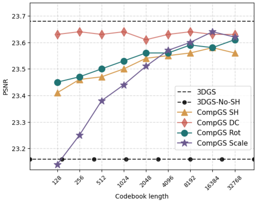
Effect of codebook size: Fig. 5 shows the effect of codebook size for quantization of different Gaussian parameters on the Tanks&Temples dataset. The DC component of color has the smallest drop in performance upon quantization and achieves results similar to the non-quantized version with as few as cluster centers. The harmonics (SH) components of color lead to a much bigger drop at lower number of clusters and improve as more clusters are added. Note that CompGS with only SH components is nearly the same size as 3DGS-No-SH but has better performance ( for ours vs. for 3DGS-No-SH ). The covariance parameters (rotation and scale) have a drop in performance at a codebook size of but improve as the codebook size is increased.
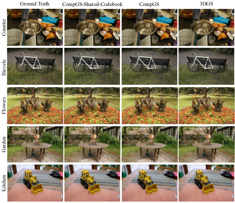
Generalization of codebook across scenes
We train our train our method
on a single scene (‘Counter’) of the Mip-NeRF360 dataset. We then freeze the codebook and calculate only assignments for the rest of the eight scenes in the dataset and report the averaged performance metrics over all scenes (Fig. 5). Interestingly, we observe that the shared codebook generalizes well across all scenes with a small drop in performance compared to learning a codebook for each scene. Sharing learnt codebook can further reduce the memory requirement and can help speed up the training of CompGS. The quality of the codebook can be improved by learning it over multiple scenes.
Conclusion:
3D Gaussian Splatting efficiently models 3D radiance fields, outperforming NeRF in learning and rendering efficiency at the cost of increased storage. To reduce storage demands, we apply opacity regularization and K-means-based vector quantization, compressing indices and employing a compact codebook. Our method cuts the storage cost of 3DGS by almost , increases rendering FPS by while maintaining image quality across benchmarks.
Acknowledgments: This work is partially funded by NSF grant 1845216 and DARPA Contract No. HR00112190135 and HR00112290115.
References
- [1] Official code repository of 3d gaussian splatting for real-time radiance field rendering. https://github.com/graphdeco-inria/gaussian-splatting
- [2] Abbasi Koohpayegani, S., Tejankar, A., Pirsiavash, H.: Compress: Self-supervised learning by compressing representations. Advances in Neural Information Processing Systems 33, 12980–12992 (2020)
- [3] Ba, L.J., Caruana, R.: Do deep nets really need to be deep? arXiv preprint arXiv:1312.6184 (2013)
- [4] Barron, J.T., Mildenhall, B., Verbin, D., Srinivasan, P.P., Hedman, P.: Mip-nerf 360: Unbounded anti-aliased neural radiance fields. In: Proceedings of the IEEE/CVF Conference on Computer Vision and Pattern Recognition. pp. 5470–5479 (2022)
- [5] Baruch, G., Chen, Z., Dehghan, A., Dimry, T., Feigin, Y., Fu, P., Gebauer, T., Joffe, B., Kurz, D., Schwartz, A., Shulman, E.: Arkitscenes - a diverse real-world dataset for 3d indoor scene understanding using mobile rgb-d data. In: NeurIPS (2021), https://arxiv.org/pdf/2111.08897.pdf
- [6] Baruch, G., Chen, Z., Dehghan, A., Feigin, Y., Fu, P., Gebauer, T., Kurz, D., Dimry, T., Joffe, B., Schwartz, A., Shulman, E.: ARKitscenes: A diverse real-world dataset for 3d indoor scene understanding using mobile RGB-d data. In: Thirty-fifth Conference on Neural Information Processing Systems Datasets and Benchmarks Track (Round 1) (2021), https://openreview.net/forum?id=tjZjv_qh_CE
- [7] Bengio, Y., Léonard, N., Courville, A.: Estimating or propagating gradients through stochastic neurons for conditional computation. arXiv preprint arXiv:1308.3432 (2013)
- [8] Chen, A., Xu, Z., Geiger, A., Yu, J., Su, H.: Tensorf: Tensorial radiance fields. In: European Conference on Computer Vision. pp. 333–350. Springer (2022)
- [9] Chen, G., Choi, W., Yu, X., Han, T., Chandraker, M.: Learning efficient object detection models with knowledge distillation. In: Proceedings of the 31st International Conference on Neural Information Processing Systems. pp. 742–751 (2017)
- [10] Chen, Z., Funkhouser, T., Hedman, P., Tagliasacchi, A.: Mobilenerf: Exploiting the polygon rasterization pipeline for efficient neural field rendering on mobile architectures. In: Proceedings of the IEEE/CVF Conference on Computer Vision and Pattern Recognition. pp. 16569–16578 (2023)
- [11] Cho, M., Vahid, K.A., Fu, Q., Adya, S., Del Mundo, C.C., Rastegari, M., Naik, D., Zatloukal, P.: edkm: An efficient and accurate train-time weight clustering for large language models. arXiv preprint arXiv:2309.00964 (2023)
- [12] Cosman, P.C., Oehler, K.L., Riskin, E.A., Gray, R.M.: Using vector quantization for image processing. Proceedings of the IEEE 81(9), 1326–1341 (1993)
- [13] Deng, C.L., Tartaglione, E.: Compressing explicit voxel grid representations: fast nerfs become also small. In: Proceedings of the IEEE/CVF Winter Conference on Applications of Computer Vision. pp. 1236–1245 (2023)
- [14] Dettmers, T., Lewis, M., Belkada, Y., Zettlemoyer, L.: Llm. int8 (): 8-bit matrix multiplication for transformers at scale. arXiv preprint arXiv:2208.07339 (2022)
- [15] Equitz, W.H.: A new vector quantization clustering algorithm. IEEE transactions on acoustics, speech, and signal processing 37(10), 1568–1575 (1989)
- [16] Fan, Z., Wang, K., Wen, K., Zhu, Z., Xu, D., Wang, Z.: Lightgaussian: Unbounded 3d gaussian compression with 15x reduction and 200+ fps. arXiv preprint arXiv:2311.17245 (2023)
- [17] Flynn, J., Neulander, I., Philbin, J., Snavely, N.: Deepstereo: Learning to predict new views from the world’s imagery. In: Proceedings of the IEEE conference on computer vision and pattern recognition. pp. 5515–5524 (2016)
- [18] Fridovich-Keil, S., Yu, A., Tancik, M., Chen, Q., Recht, B., Kanazawa, A.: Plenoxels: Radiance fields without neural networks. In: Proceedings of the IEEE/CVF Conference on Computer Vision and Pattern Recognition. pp. 5501–5510 (2022)
- [19] Garbin, S.J., Kowalski, M., Johnson, M., Shotton, J., Valentin, J.: Fastnerf: High-fidelity neural rendering at 200fps. In: Proceedings of the IEEE/CVF International Conference on Computer Vision. pp. 14346–14355 (2021)
- [20] Gersho, A., Gray, R.M.: Vector quantization and signal compression, vol. 159. Springer Science & Business Media (2012)
- [21] Girish, S., Gupta, K., Shrivastava, A.: Eagles: Efficient accelerated 3d gaussians with lightweight encodings. arXiv preprint arXiv:2312.04564 (2023)
- [22] Gong, Y., Liu, L., Yang, M., Bourdev, L.: Compressing deep convolutional networks using vector quantization. arXiv preprint arXiv:1412.6115 (2014)
- [23] Gray, R.: Vector quantization. IEEE Assp Magazine 1(2), 4–29 (1984)
- [24] Gu, S., Chen, D., Bao, J., Wen, F., Zhang, B., Chen, D., Yuan, L., Guo, B.: Vector quantized diffusion model for text-to-image synthesis. In: Proceedings of the IEEE/CVF Conference on Computer Vision and Pattern Recognition. pp. 10696–10706 (2022)
- [25] Gupta, S., Agrawal, A., Gopalakrishnan, K., Narayanan, P.: Deep learning with limited numerical precision. In: International conference on machine learning. pp. 1737–1746. PMLR (2015)
- [26] Han, S., Mao, H., Dally, W.J.: Deep compression: Compressing deep neural networks with pruning, trained quantization and huffman coding. arXiv preprint arXiv:1510.00149 (2015)
- [27] Hedman, P., Philip, J., Price, T., Frahm, J.M., Drettakis, G., Brostow, G.: Deep blending for free-viewpoint image-based rendering. ACM Transactions on Graphics (ToG) 37(6), 1–15 (2018)
- [28] Hedman, P., Srinivasan, P.P., Mildenhall, B., Barron, J.T., Debevec, P.: Baking neural radiance fields for real-time view synthesis. In: Proceedings of the IEEE/CVF International Conference on Computer Vision. pp. 5875–5884 (2021)
- [29] Henzler, P., Mitra, N.J., Ritschel, T.: Escaping plato’s cave: 3d shape from adversarial rendering. In: Proceedings of the IEEE/CVF International Conference on Computer Vision. pp. 9984–9993 (2019)
- [30] Hinton, G., Vinyals, O., Dean, J.: Distilling the knowledge in a neural network. arXiv preprint arXiv:1503.02531 (2015)
- [31] Huang, B., Yan, X., Chen, A., Gao, S., Yu, J.: Pref: Phasorial embedding fields for compact neural representations. arXiv preprint arXiv:2205.13524 (2022)
- [32] Jacob, B., Kligys, S., Chen, B., Zhu, M., Tang, M., Howard, A., Adam, H., Kalenichenko, D.: Quantization and training of neural networks for efficient integer-arithmetic-only inference. In: Proceedings of the IEEE Conference on Computer Vision and Pattern Recognition. pp. 2704–2713 (2018)
- [33] Kerbl, B., Kopanas, G., Leimkühler, T., Drettakis, G.: 3d gaussian splatting for real-time radiance field rendering. ACM Transactions on Graphics (ToG) 42(4), 1–14 (2023)
- [34] Knapitsch, A., Park, J., Zhou, Q.Y., Koltun, V.: Tanks and temples: Benchmarking large-scale scene reconstruction. ACM Transactions on Graphics (ToG) 36(4), 1–13 (2017)
- [35] Krishnamoorthi, R.: Quantizing deep convolutional networks for efficient inference: A whitepaper. arXiv preprint arXiv:1806.08342 (2018)
- [36] Lee, J.C., Rho, D., Sun, X., Ko, J.H., Park, E.: Compact 3d gaussian representation for radiance field. arXiv preprint arXiv:2311.13681 (2023)
- [37] Lee, J.C., Rho, D., Sun, X., Ko, J.H., Park, E.: Compact 3d gaussian representation for radiance field. In: Proceedings of the IEEE/CVF Conference on Computer Vision and Pattern Recognition. pp. 21719–21728 (2024)
- [38] Lee, Y.Y., Woods, J.W.: Motion vector quantization for video coding. IEEE Transactions on Image Processing 4(3), 378–382 (1995)
- [39] Li, L., Shen, Z., Wang, Z., Shen, L., Bo, L.: Compressing volumetric radiance fields to 1 mb. In: Proceedings of the IEEE/CVF Conference on Computer Vision and Pattern Recognition. pp. 4222–4231 (2023)
- [40] Li, L., Shen, Z., Wang, Z., Shen, L., Tan, P.: Streaming radiance fields for 3d video synthesis. Advances in Neural Information Processing Systems 35, 13485–13498 (2022)
- [41] Ling, L., Sheng, Y., Tu, Z., Zhao, W., Xin, C., Wan, K., Yu, L., Guo, Q., Yu, Z., Lu, Y., et al.: Dl3dv-10k: A large-scale scene dataset for deep learning-based 3d vision. arXiv preprint arXiv:2312.16256 (2023)
- [42] Makhoul, J., Roucos, S., Gish, H.: Vector quantization in speech coding. Proceedings of the IEEE 73(11), 1551–1588 (1985)
- [43] Mildenhall, B., Srinivasan, P.P., Tancik, M., Barron, J.T., Ramamoorthi, R., Ng, R.: Nerf: Representing scenes as neural radiance fields for view synthesis. In: Proceedings of the European Conference on Computer Vision (ECCV) (2020), http://arxiv.org/abs/2003.08934v2
- [44] Morgenstern, W., Barthel, F., Hilsmann, A., Eisert, P.: Compact 3d scene representation via self-organizing gaussian grids. arXiv preprint arXiv:2312.13299 (2023)
- [45] Müller, T., Evans, A., Schied, C., Keller, A.: Instant neural graphics primitives with a multiresolution hash encoding. ACM Transactions on Graphics (ToG) 41(4), 1–15 (2022)
- [46] Niedermayr, S., Stumpfegger, J., Westermann, R.: Compressed 3d gaussian splatting for accelerated novel view synthesis. arXiv preprint arXiv:2401.02436 (2023)
- [47] Niedermayr, S., Stumpfegger, J., Westermann, R.: Compressed 3d gaussian splatting for accelerated novel view synthesis. In: Proceedings of the IEEE/CVF Conference on Computer Vision and Pattern Recognition. pp. 10349–10358 (2024)
- [48] Nooralinejad, P., Abbasi, A., Koohpayegani, S.A., Meibodi, K.P., Khan, R.M.S., Kolouri, S., Pirsiavash, H.: Pranc: Pseudo random networks for compacting deep models. In: Proceedings of the IEEE/CVF International Conference on Computer Vision. pp. 17021–17031 (2023)
- [49] Peng, S., Jiang, C., Liao, Y., Niemeyer, M., Pollefeys, M., Geiger, A.: Shape as points: A differentiable poisson solver. Advances in Neural Information Processing Systems 34, 13032–13044 (2021)
- [50] Penner, E., Zhang, L.: Soft 3d reconstruction for view synthesis. ACM Transactions on Graphics (TOG) 36(6), 1–11 (2017)
- [51] Polino, A., Pascanu, R., Alistarh, D.: Model compression via distillation and quantization. arXiv preprint arXiv:1802.05668 (2018)
- [52] Rastegari, M., Ordonez, V., Redmon, J., Farhadi, A.: Xnor-net: Imagenet classification using binary convolutional neural networks (2016)
- [53] Rastegari, M., Ordonez, V., Redmon, J., Farhadi, A.: Xnor-net: Imagenet classification using binary convolutional neural networks. In: Leibe, B., Matas, J., Sebe, N., Welling, M. (eds.) Computer Vision - ECCV 2016 - 14th European Conference, Amsterdam, The Netherlands, October 11-14, 2016, Proceedings, Part IV. Lecture Notes in Computer Science, vol. 9908, pp. 525–542. Springer (2016). https://doi.org/10.1007/978-3-319-46493-0_32, https://doi.org/10.1007/978-3-319-46493-0_32
- [54] Razavi, A., Van den Oord, A., Vinyals, O.: Generating diverse high-fidelity images with vq-vae-2. Advances in neural information processing systems 32 (2019)
- [55] Reiser, C., Peng, S., Liao, Y., Geiger, A.: Kilonerf: Speeding up neural radiance fields with thousands of tiny mlps. In: Proceedings of the IEEE/CVF International Conference on Computer Vision. pp. 14335–14345 (2021)
- [56] Riegler, G., Koltun, V.: Free view synthesis. In: Computer Vision–ECCV 2020: 16th European Conference, Glasgow, UK, August 23–28, 2020, Proceedings, Part XIX 16. pp. 623–640. Springer (2020)
- [57] Schwarz, K., Sauer, A., Niemeyer, M., Liao, Y., Geiger, A.: Voxgraf: Fast 3d-aware image synthesis with sparse voxel grids. Advances in Neural Information Processing Systems 35, 33999–34011 (2022)
- [58] Sitzmann, V., Thies, J., Heide, F., Nießner, M., Wetzstein, G., Zollhofer, M.: Deepvoxels: Learning persistent 3d feature embeddings. In: Proceedings of the IEEE/CVF Conference on Computer Vision and Pattern Recognition. pp. 2437–2446 (2019)
- [59] Sun, C., Sun, M., Chen, H.T.: Direct voxel grid optimization: Super-fast convergence for radiance fields reconstruction. In: Proceedings of the IEEE/CVF Conference on Computer Vision and Pattern Recognition. pp. 5459–5469 (2022)
- [60] Takikawa, T., Evans, A., Tremblay, J., Müller, T., McGuire, M., Jacobson, A., Fidler, S.: Variable bitrate neural fields. In: ACM SIGGRAPH 2022 Conference Proceedings. pp. 1–9 (2022)
- [61] Tang, J., Chen, X., Wang, J., Zeng, G.: Compressible-composable nerf via rank-residual decomposition. In: Advances in Neural Information Processing Systems (2022)
- [62] Thies, J., Zollhöfer, M., Nießner, M.: Deferred neural rendering: Image synthesis using neural textures. Acm Transactions on Graphics (TOG) 38(4), 1–12 (2019)
- [63] Van Den Oord, A., Vinyals, O., et al.: Neural discrete representation learning. Advances in neural information processing systems 30 (2017)
- [64] Vanhoucke, V., Senior, A., Mao, M.Z.: Improving the speed of neural networks on cpus (2011)
- [65] Wang, L., Zhang, J., Liu, X., Zhao, F., Zhang, Y., Zhang, Y., Wu, M., Yu, J., Xu, L.: Fourier plenoctrees for dynamic radiance field rendering in real-time. In: Proceedings of the IEEE/CVF Conference on Computer Vision and Pattern Recognition. pp. 13524–13534 (2022)
- [66] Wen, W., Wu, C., Wang, Y., Chen, Y., Li, H.: Learning structured sparsity in deep neural networks. arXiv preprint arXiv:1608.03665 (2016)
- [67] Wu, X., Xu, J., Zhu, Z., Bao, H., Huang, Q., Tompkin, J., Xu, W.: Scalable neural indoor scene rendering. ACM Transactions on Graphics (TOG) (2022)
- [68] Xu, Q., Xu, Z., Philip, J., Bi, S., Shu, Z., Sunkavalli, K., Neumann, U.: Point-nerf: Point-based neural radiance fields. In: Proceedings of the IEEE/CVF Conference on Computer Vision and Pattern Recognition. pp. 5438–5448 (2022)
- [69] Yu, A., Li, R., Tancik, M., Li, H., Ng, R., Kanazawa, A.: Plenoctrees for real-time rendering of neural radiance fields. In: Proceedings of the IEEE/CVF International Conference on Computer Vision. pp. 5752–5761 (2021)
- [70] Zhou, T., Tulsiani, S., Sun, W., Malik, J., Efros, A.A.: View synthesis by appearance flow. In: Computer Vision–ECCV 2016: 14th European Conference, Amsterdam, The Netherlands, October 11–14, 2016, Proceedings, Part IV 14. pp. 286–301. Springer (2016)
Appendix
Here, we compare the performance of our CompGS with state-of-the-art approaches on the NeRF-Synthetic dataset (Section E). Section F shows exploratory results on generalization of the learnt vector codebook across scenes and Section G provides insights on the learnt codebook assignments. We also provide scene-wise results (section H), ablations on baselines (section I) and additional visualizations and qualitative comparisons on the ARKit-200 dataset (section J).
E Results on NeRF-Synthetic dataset
The results (PSNR) for the NeRF-Synthetic dataset [43] are presented in Table E.10. Our CompGS approach achieves an impressive average improvement of points in PSNR compared to the 3DGS-No-SH baseline while using less than half its memory. As reported in the main submission, we report metrics for 3DGS both from the original paper and using our own runs. We observe an improvement for 3DGS [33] over their official reported numbers by points.
| Mic | Chair | Ship | Materials | Lego | Drums | Ficus | Hotdog | Avg. | |
| Plenoxels | 33.26 | 33.98 | 29.62 | 29.14 | 34.10 | 25.35 | 31.83 | 36.81 | 31.76 |
| INGP-Base | 36.22 | 35.00 | 31.10 | 29.78 | 36.39 | 26.02 | 33.51 | 37.40 | 33.18 |
| Mip-Nerf | 36.51 | 35.14 | 30.41 | 30.71 | 35.70 | 25.48 | 33.29 | 37.48 | 33.09 |
| Point-NeRF | 35.95 | 35.40 | 30.97 | 29.61 | 35.04 | 26.06 | 36.13 | 37.30 | 33.30 |
| 3DGS | 35.36 | 35.83 | 30.80 | 30.00 | 35.78 | 26.15 | 34.87 | 37.72 | 33.32 |
| 3DGS∗ | 36.80 | 35.51 | 31.69 | 30.48 | 36.06 | 26.28 | 35.49 | 38.06 | 33.80 |
| 3DGS-No-SH | 34.37 | 34.09 | 29.86 | 28.42 | 34.84 | 25.48 | 32.30 | 36.43 | 31.97 |
| CompGS 4k | 35.99 | 34.92 | 31.05 | 29.74 | 35.09 | 25.93 | 35.04 | 37.04 | 33.10 |
F Generalization of codebook across scenes
We train our vector quantization approach including the codebook and the code assignments on a single scene (‘Counter’) of the Mip-NeRF360 dataset. We then freeze the codebook and learn only assignments for the rest of the eight scenes in the dataset and report the averaged performance metrics over all scenes. In addition to the results in Fig.5 of the main submission, we provide results with our 32K variant here in table F.11. Interestingly, we observe that the shared codebook generalizes well across all scenes with a small drop in performance compared to learning a codebook for each scene. Sharing learnt codebook can further reduce the memory requirement and can help speed up the training of CompGS. The quality of the codebook can be improved by learning it over multiple scenes. Fig. J.8 shows qualitative comparison of the same. There are no apparent differences between CompGS and CompGS-Shared-Codebook approaches.
| Dataset | Mip-NeRF360 | ||
| Method | SSIM↑ | PSNR↑ | LPIPS↓ |
| 3DGS | 0.815 | 27.21 | 0.214 |
| 3DGS ∗ | 0.813 | 27.42 | 0.217 |
| CompGS 4K | 0.804 | 26.97 | 0.234 |
| CompGS 32K | 0.806 | 27.12 | 0.240 |
| CompGS Shared Codebook 4K | 0.797 | 26.64 | 0.242 |
| CompGS Shared Codebook 32K | 0.800 | 26.780 | 0.247 |
G Analysis of learnt code assignments
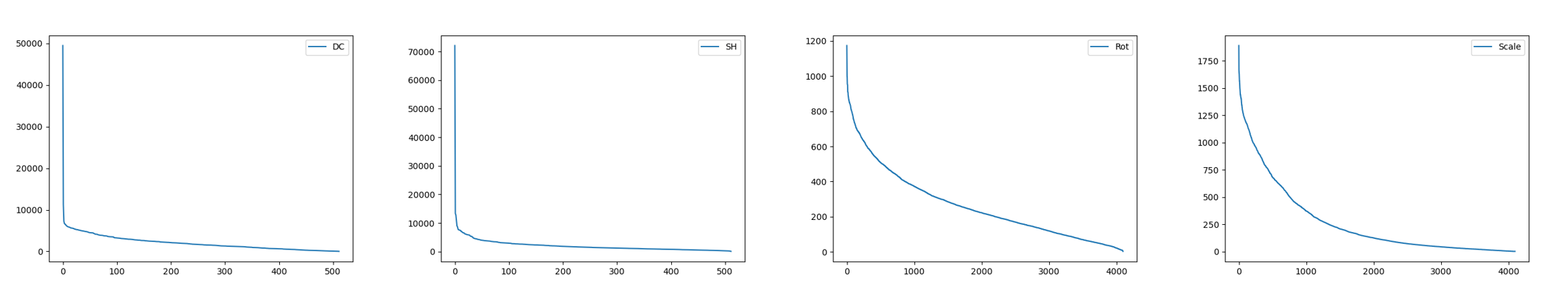
In Fig. G.6, we plot the sorted histogram of the code assignments (cluster to which each Gaussian belongs to) for each parameter on the ‘Train’ scene of Tanks&Temples dataset. We observe that just a single code out of the in total is assigned to nearly of the Gaussians for both the SH and DC parameters. Similarly, a few clusters dominate even in the case of rotation and scale parameters, albeit to a lower extent. Such a non-uniform distribution of cluster sizes suggest that further compression can be achieved by using Huffman coding to store the assignment indices.
H Scene-wise Metrics
For brevity, we reported the averaged metrics over all scenes in a dataset in our main submission. Here in table H.12, we provide the detailed scene-wise metrics for MipNerf-360, Tanks and Temples and DeepBlending datasets.
| Scene | Method | SSIM↑ | PSNR↑ | LPIPS↓ | Train Time(s) | FPS | Mem(MB) | #Gauss |
| Bicycle | 3DGS | 0.763 | 25.169 | 0.212 | 1845 | 68 | 1422 | 6026079 |
| CompGS 32K | 0.755 | 25.068 | 0.244 | 2123 | 242 | 29 | 1314018 | |
| Bonsai | 3DGS | 0.940 | 31.918 | 0.206 | 876 | 276 | 293 | 1241520 |
| CompGS 32K | 0.932 | 31.195 | 0.223 | 1405 | 492 | 10 | 377227 | |
| Counter | 3DGS | 0.906 | 29.018 | 0.202 | 968 | 208 | 283 | 1200091 |
| CompGS 32K | 0.895 | 28.467 | 0.222 | 1571 | 356 | 10 | 385515 | |
| Flowers | 3DGS | 0.602 | 21.456 | 0.339 | 1192 | 133 | 851 | 3605827 |
| CompGS 32K | 0.588 | 21.262 | 0.367 | 1744 | 343 | 23 | 1037132 | |
| Garden | 3DGS | 0.863 | 27.241 | 0.108 | 1870 | 76 | 1347 | 5709543 |
| CompGS 32K | 0.848 | 26.822 | 0.140 | 2177 | 258 | 30 | 1370624 | |
| Kitchen | 3DGS | 0.926 | 31.510 | 0.127 | 1206 | 158 | 425 | 1801403 |
| CompGS 32K | 0.918 | 30.774 | 0.142 | 1729 | 317 | 13 | 564382 | |
| Room | 3DGS | 0.917 | 31.346 | 0.221 | 1020 | 190 | 364 | 1541909 |
| CompGS 32K | 0.912 | 31.131 | 0.235 | 1439 | 444 | 9 | 327191 | |
| Stump | 3DGS | 0.772 | 26.651 | 0.215 | 1445 | 104 | 1136 | 4815087 |
| CompGS 32K | 0.770 | 26.605 | 0.236 | 1936 | 303 | 27 | 1226044 | |
| Treehill | 3DGS | 0.633 | 22.504 | 0.327 | 1213 | 122 | 879 | 3723675 |
| CompGS 32K | 0.634 | 22.747 | 0.355 | 1744 | 336 | 23 | 1002290 | |
| Train | 3DGS | 0.811 | 21.991 | 0.209 | 563 | 253 | 254 | 1077461 |
| CompGS 32K | 0.804 | 21.789 | 0.231 | 1169 | 456 | 12 | 500811 | |
| Truck | 3DGS | 0.878 | 25.385 | 0.148 | 897 | 159 | 611 | 2588966 |
| CompGS 32K | 0.872 | 25.092 | 0.165 | 1306 | 494 | 13 | 540081 | |
| DrJohnson | 3DGS | 0.898 | 29.089 | 0.247 | 1312 | 121 | 772 | 3270679 |
| CompGS 32K | 0.906 | 29.445 | 0.249 | 1717 | 379 | 17 | 714902 | |
| Playroom | 3DGS | 0.901 | 29.903 | 0.246 | 1003 | 181 | 551 | 2335846 |
| CompGS 32K | 0.908 | 30.347 | 0.253 | 1422 | 589 | 10 | 393414 |
I Ablations for Gaussian count reduction
We perform ablations to choose the right hyperparameters for the baseline approaches to reduce the Gaussian count. The metrics for the chosen settings are reported in table 3 of the main submission. The ablations for minimum opacity, densification interval and end iteration and gradient threshold are shown in tables I.13, I.14, I.15 and I.16 espectively. Among these baselines, modify gradient threshold provides the best trade-off between model size and performance.
| Mip-NeRF360 | Tanks&Temples | Deep Blending | ||||||||||
| SSIM | PSNR | LPIPS | #Gauss | SSIM | PSNR | LPIPS | #Gauss | SSIM | PSNR | LPIPS | #Gauss | |
| 0.05 | 0.810 | 27.308 | 0.230 | 1.93M | 0.839 | 23.508 | 0.194 | 1.04M | 0.902 | 29.542 | 0.251 | 1.47M |
| 0.1 | 0.802 | 27.120 | 0.244 | 1.46M | 0.833 | 23.439 | 0.204 | 780K | 0.902 | 29.504 | 0.255 | 1.01M |
| Mip-NeRF360 | Tanks&Temples | Deep Blending | ||||||||||
| SSIM | PSNR | LPIPS | #Gauss | SSIM | PSNR | LPIPS | #Gauss | SSIM | PSNR | LPIPS | #Gauss | |
| 300 | 0.803 | 27.201 | 0.241 | 1.70M | 0.837 | 23.517 | 0.195 | 1.00M | 0.902 | 29.705 | 0.253 | 1.30M |
| 500 | 0.794 | 26.98 | 0.255 | 1.07M | 0.832 | 23.36 | 0.206 | 709K | 0.902 | 29.76 | 0.258 | 844K |
| Mip-NeRF360 | Tanks&Temples | Deep Blending | ||||||||||
| SSIM | PSNR | LPIPS | #Gauss | SSIM | PSNR | LPIPS | #Gauss | SSIM | PSNR | LPIPS | #Gauss | |
| 5000 | 0.797 | 27.199 | 0.241 | 1.92M | 0.838 | 23.599 | 0.188 | 1.12M | 0.897 | 29.486 | 0.256 | 1.34M |
| 3000 | 0.780 | 27.02 | 0.267 | 1.12M | 0.835 | 23.55 | 0.194 | 810K | 0.896 | 29.42 | 0.264 | 795K |
| Mip-NeRF360 | Tanks&Temples | Deep Blending | ||||||||||
| SSIM | PSNR | LPIPS | #Gauss | SSIM | PSNR | LPIPS | #Gauss | SSIM | PSNR | LPIPS | #Gauss | |
| 0.00035 | 0.786 | 26.934 | 0.265 | 1.27M | 0.833 | 23.579 | 0.203 | 833K | 0.901 | 29.574 | 0.254 | 1.41M |
| 0.00045 | 0.769 | 26.57 | 0.292 | 809K | 0.825 | 23.31 | 0.217 | 578K | 0.900 | 29.49 | 0.260 | 1.01M |
| 0.00055 | 0.754 | 26.290 | 0.312 | 552K | 0.818 | 23.041 | 0.228 | 433K | 0.899 | 29.544 | 0.265 | 764K |
J Qualitative comparison on ARKit-200 dataset.