Competition on Dynamic Optimization Problems Generated by Generalized Moving Peaks Benchmark (GMPB)
Abstract
The Generalized Moving Peaks Benchmark (GMPB) [1] is a tool for generating continuous dynamic optimization problem instances with controllable dynamic and morphological characteristics. GMPB has been used in recent Competitions on Dynamic Optimization at prestigious conferences, such as the IEEE Congress on Evolutionary Computation (CEC). This dynamic benchmark generator can create a wide variety of landscapes, ranging from simple unimodal to highly complex multimodal configurations, and from symmetric to asymmetric forms. It also supports diverse surface textures, from smooth to highly irregular, and can generate varying levels of variable interaction and conditioning. This document provides an overview of GMPB, emphasizing how its parameters can be adjusted to produce landscapes with customizable characteristics. The MATLAB implementation of GMPB is available on the EDOLAB platform [2].
Index Terms:
Evolutionary dynamic optimization, Tracking moving optimum, Dynamic optimization problems, Generalized moving peaks benchmark.I Introduction
Search spaces of many real-world optimization problems are dynamic in terms of the objective function, the number of variables, and/or constraints [3, 4]. Optimization problems that change over time and need to be solved online by an optimization method are referred to as dynamic optimization problems (DOPs) [5]. To solve DOPs, algorithms not only need to find desirable solutions but also to react to the environmental changes in order to quickly find a new solution when the previous one becomes suboptimal [6].
To comprehensively evaluate the effectiveness of algorithms designed for DOPs, a suitable benchmark generator is crucial. Commonly used and well-known benchmark generators in this domain use the idea of having several components that form the landscape. In most existing DOP benchmarks, the width, height, and location of these components change over time [7]. One of the benchmark generators that is designed based on this idea is the Moving Peaks Benchmark (MPB) [8], which is the most widely used synthetic problem in the DOP field [7, 6, 4]. Each component in MPB is formed by usually a simple peak whose basin of attraction is determined using a function.
Despite the popularity of the traditional MPB, landscapes generated by this benchmark consist of components that are smooth/regular, symmetric, unimodal, separable [9], and easy-to-optimize, which may not be the case in many real-world problems. In [1], a generalized MPB (GMPB) is proposed which can generate components with a variety of characteristics that can range from unimodal to highly multimodal, from symmetric to highly asymmetric, from smooth to highly irregular, and with different variable interaction degrees and condition numbers. GMPB is a benchmark generator with fully controllable features that helps researchers to analyze DOP algorithms and investigate their effectiveness in facing a variety of different problem characteristics.
II Generalized Moving Peaks Benchmark [1]
The baseline function of GMPB is111Herein, we focus on fully non-separable problem instances which are constructed by Eq. (1). Those readers who are interested in partially/fully separable problems (i.e., composition based functions), refer to [1].:
| (1) |
where is calculated as:
| (2) |
where is a solution in -dimensional space, is the number of components, is the rotation matrix of th component in the th environment, is a diagonal matrix whose diagonal elements show the width of th component in different dimensions, is th dimension of , and and are irregularity parameters of the th component.
For each component , the rotation matrix is obtained by rotating the projection of onto all - planes by a given angle . The total number of unique planes which will be rotated is . For rotating each - plane by a certain angle (), a Givens rotation matrix must be constructed. To this end, first, is initialized to an identity matrix ; then, four elements of are altered as:
| (3) | ||||
| (4) | ||||
| (5) | ||||
| (6) |
where is the element at th row and th column of . in the th environment is calculated by:
| (7) |
where contains all unique pairs of dimensions defining all possible planes in a -dimensional space. The order of the multiplications of the Givens rotation matrices is random. The reason behind using (7) for calculating is that we aim to have control on the rotation matrix based on an angle severity . Note that the initial for problem instances with rotation property is obtained by using the Gram-Schmidt orthogonalization method on a matrix with normally distributed entries.
For each component , the height, width vector, center, angle, and irregularity parameters change from one environment to the next according to the following update rules:
| (8) | ||||
| (9) | ||||
| (10) | ||||
| (11) | ||||
| (12) | ||||
| (13) |
where is a random number drawn from a Gaussian distribution with mean 0 and variance 1, shows the vector of center position of the th component, is a -dimensional vector of random numbers generated by , is the Euclidean length (i.e., -norm) of , generates a unit vector with a random direction, , , , , , and are height, width, shift, angle, and two irregularity parameters’ change severity values, respectively, shows the width of the th component in the th dimension, and and show the height and angle of the th component, respectively.
Outputs of equations (8) to (13) are bounded as follows: , , , , , and , where and are maximum and minimum problem space bounds. For keeping the above mentioned values in their bounds, a Reflect method is utilized. Assume represents one of the equations (8) to (13). The output based on the reflect method is:
| (14) |
II-A Problem characteristics
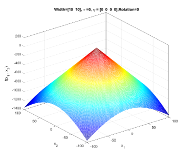
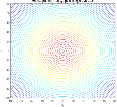
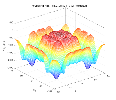
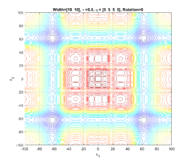
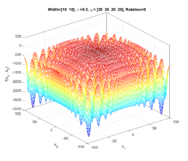
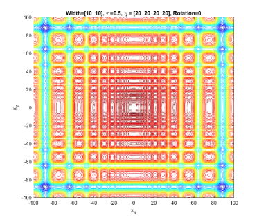
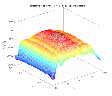
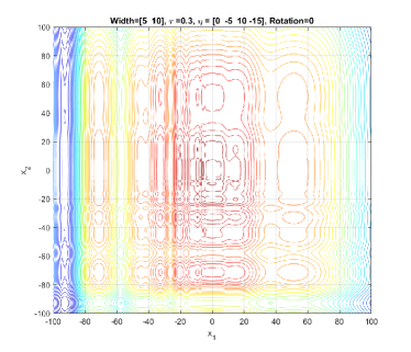
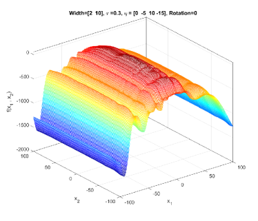
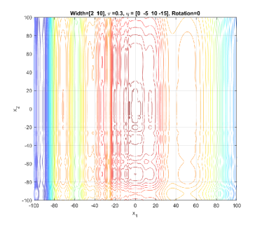
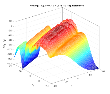
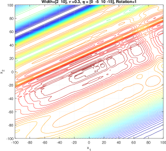
In this section, we describe the main characteristics of the components and the landscapes generated by GMPB. Note that in the 2-dimensional examples provided in this part, the values of width (2-dimensional vector), irregularity parameters ( and four values for ), and rotation status (1 is rotated and 0 otherwise) are shown in the title of figures.
II-A1 Component characteristics
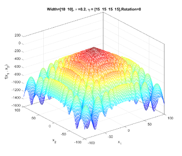
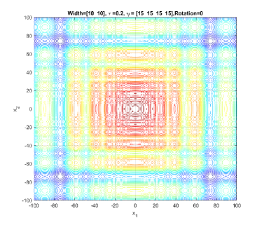
In the simplest form, (1) generates a symmetric, unimodal, smooth/regular, and easy-to-optimize conical peak (see Figure 1). By setting different values to and , a component generated by GMPB can become irregular and multimodal. Figure 2 shows three irregular and multimodal components generated by GMPB with different parameter settings for and . A component is symmetric when all values are identical, and components whose values are set to different values are asymmetric (see Figure 3).
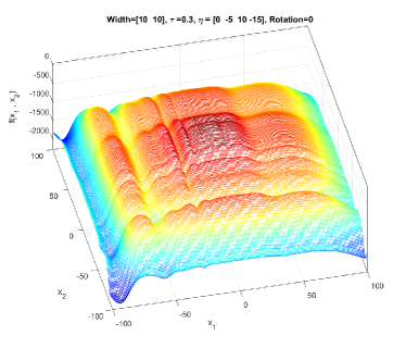
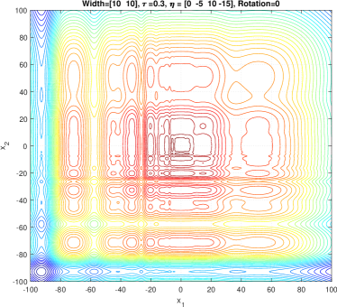
GMPB is capable of generating components with various condition numbers. A component generated by GMPB has a width value in each dimension. When the width values of a component are identical in all dimensions, the condition number of the component will be one, i.e., it is not ill-conditioned. The condition number of a component is the ratio of its largest width value to its smallest value [1]. If a component’s width value is stretched in one axis’s direction more than the other axes, then, the component is ill-conditioned. Figure 4 depicts three ill-conditioned components.
II-A2 Search space characteristics
Landscapes generated by GMPB are constructed by assembling several components using a function in (1), which determines the basin of attraction of each component. As shown in [9], a landscape consists of several components (i.e., ) is fully non-separable. Figure 5 shows a landscape with five components.


III Parameter settings
Table I shows the parameter settings of GMPB. By changing the number of dimensions, shift severity value, the number of components, and change frequency, the difficulty level of the generated problem instances can be adjusted. Every fitness evaluations, the center position, height, width vector, angle, and irregularity parameters of each component change using the dynamics presented in (8) to (13).
| Parameter | Symbol | Value(s) |
|---|---|---|
| Dimension | 2,5,10,20 | |
| Shift severity | 1,2,5 | |
| Numbers of components | 1,5,10,25,50,100,200 | |
| Angle severity | ||
| Height severity | 7 | |
| Width severity | 1 | |
| Irregularity parameter severity | 0.2 | |
| Irregularity parameter severity | 10 | |
| Search range | ||
| Height range | ||
| Width range | ||
| Angle range | ||
| Irregularity parameter range | ||
| Irregularity parameter range | ||
| Initial center position | ||
| Initial height | ||
| Initial width | ||
| Initial angle | ||
| Initial irregularity parameter | ||
| Initial irregularity parameter | ||
| Initial rotation matrix | ||
| Change frequency | 1000,2500,5000,10000 | |
| Number of Environments | 100 |
-
is initialized by performing the Gram-Schmidt orthogonalization method on a matrix with normally distributed entries.
IV Performance indicator
To measure the performance of algorithms in solving the problem instances generated by GMPB, the offline-error [10] () and the average error of the best found solution in all environments, i.e., the best error before change, () [11] are used as the performance indicators. is the most commonly used performance indicator in the literature [12]. This approach calculates the average error of the best found position over all fitness evaluations using the following equation:
| (15) |
where is the global optimum position at the th environment, is the number of environments, is the change frequency, is the fitness evaluation counter for each environment, and is the best found position at the th fitness evaluation in the th environment.
is the second commonly used performance indicator in the field [12]. only considers the last error before each environmental change (i.e., at the end of each environment):
| (16) |
where is the best found position in th environment which is fetched at the end of the th environment.
V Source code
GMPB is a featured component of EDOLAB [2], a comprehensive MATLAB222Version R2020b and later optimization platform designed for both educational and experimental purposes in dynamic environments. EDOLAB hosts an array of 25 evolutionary dynamic optimization algorithms. Researchers are encouraged to utilize the guidelines in [2] to integrate their own algorithms into EDOLAB. This allows for an extensive evaluation of their algorithms’ performance against a variety of problem instances created by dynamic optimization benchmark generators, including GMPB. The source code of EDOLAB is readily available and can be accessed at here.
We also provided another source code that visualizes 2-dimensional landscapes generated by GMPB which can be found in [13]. Using this source code, researchers can observe the impacts of different parameter settings on morphological characteristics of the problems generated by GMPB.
References
- [1] D. Yazdani, M. N. Omidvar, R. Cheng, J. Branke, T. T. Nguyen, and X. Yao, “Benchmarking continuous dynamic optimization: Survey and generalized test suite,” IEEE Transactions on Cybernetics, pp. 1 – 14, 2020.
- [2] M. Peng, Z. She, D. Yazdani, D. Yazdani, W. Luo, C. Li, J. Branke, T. T. Nguyen, A. H. Gandomi, Y. Jin, and X. Yao, “Evolutionary dynamic optimization laboratory: A matlab optimization platform for education and experimentation in dynamic environments,” arXiv preprint arXiv:2308.12644, 2023.
- [3] T. T. Nguyen, S. Yang, and J. Branke, “Evolutionary dynamic optimization: A survey of the state of the art,” Swarm and Evolutionary Computation, vol. 6, pp. 1 – 24, 2012.
- [4] T. T. Nguyen, “Continuous dynamic optimisation using evolutionary algorithms,” Ph.D. dissertation, University of Birmingham, 2011.
- [5] D. Yazdani, R. Cheng, D. Yazdani, J. Branke, , Y. Jin, and X. Yao, “A survey of evolutionary continuous dynamic optimization over two decades – part A,” IEEE Transactions on Evolutionary Computation, 2021.
- [6] D. Yazdani, “Particle swarm optimization for dynamically changing environments with particular focus on scalability and switching cost,” Ph.D. dissertation, Liverpool John Moores University, Liverpool, UK, 2018.
- [7] C. Cruz, J. R. González, and D. A. Pelta, “Optimization in dynamic environments: a survey on problems, methods and measures,” Soft Computing, vol. 15, no. 7, pp. 1427–1448, 2011.
- [8] J. Branke, “Memory enhanced evolutionary algorithms for changing optimization problems,” in IEEE Congress on Evolutionary Computation, vol. 3. IEEE, 1999, pp. 1875–1882.
- [9] D. Yazdani, M. N. Omidvar, J. Branke, T. T. Nguyen, and X. Yao, “Scaling up dynamic optimization problems: A divide-and-conquer approach,” IEEE Transaction on Evolutionary Computation, 2019.
- [10] J. Branke and H. Schmeck, “Designing evolutionary algorithms for dynamic optimization problems,” in Advances in Evolutionary Computing, A. Ghosh and S. Tsutsui, Eds. Springer Natural Computing Series, 2003, pp. 239–262.
- [11] K. Trojanowski and Z. Michalewicz, “Searching for optima in non-stationary environments,” in Congress on Evolutionary Computation, vol. 3, 1999, pp. 1843–1850.
- [12] D. Yazdani, R. Cheng, D. Yazdani, J. Branke, , Y. Jin, and X. Yao, “A survey of evolutionary continuous dynamic optimization over two decades – part B,” IEEE Transactions on Evolutionary Computation, 2021.
- [13] D. Yazdani, Visualizing 2-D Generalized Moving Peaks Bnechmark (MATLAB Source Code), 2021 (accessed December 09, 2023). [Online]. Available: https://github.com/Danial-Yazdani/GMPB_2D_Visualization