Compatibility-aware Heterogeneous Visual Search

Rahul Duggal Hao Zhou Shuo Yang Yuanjun Xiong
Wei Xia Zhuowen Tu Stefano Soatto

AWS/Amazon AI
[email protected] {zhouho, shuoy, yuanjx, wxia, ztu, soattos}@amazon.com Currently at the Georgia Institute of Technology. Work conducted during an internship with Amazon AI.Corresponding author.

Abstract

We tackle the problem of visual search under resource constraints. Existing systems use the same embedding model to compute representations (embeddings) for the query and gallery images. Such systems inherently face a hard accuracy-efficiency trade-off: the embedding model needs to be large enough to ensure high accuracy, yet small enough to enable query-embedding computation on resource-constrained platforms. This trade-off could be mitigated if gallery embeddings are generated from a large model and query embeddings are extracted using a compact model. The key to building such a system is to ensure representation compatibility between the query and gallery models. In this paper, we address two forms of compatibility: One enforced by modifying the parameters of each model that computes the embeddings. The other by modifying the architectures that compute the embeddings, leading to compatibility-aware neural architecture search (Cmp-NAS). We test Cmp-NAS on challenging retrieval tasks for fashion images (DeepFashion2), and face images (IJB-C). Compared to ordinary (homogeneous) visual search using the largest embedding model (paragon), Cmp-NAS achieves 80-fold and 23-fold cost reduction while maintaining accuracy within $0.3\%$ and $1.6\%$ of the paragon on DeepFashion2 and IJB-C respectively.

1 Introduction

Refer to caption — Figure 1: Homogeneous visual search uses the same embedding model, either large (orange) to meet performance specifications, or small (green) to meet cost constraints, forcing a dichotomy. Heterogeneous Visual Search (blue) uses a large model to compute embeddings for the gallery, and a small model for the query images. This allows high efficiency without sacrificing accuracy, provided that the green and orange embedding models are designed and trained to be compatible.

A visual search system in an “open universe” setting is often composed of a gallery model $\phi_{g}$ and a query model $\phi_{q}$ , both mapping an input image to a vector representation known as embedding. The gallery model $\phi_{g}$ is typically used to map a set of gallery images onto their embedding vectors, a process known as indexing, while the query model extracts embeddings from query images to perform search against the indexed gallery. Most existing visual search approaches [qayyum2017medical, razavian2016visual, xie2015image, babenko2015aggregating, tolias2015particular] use the same model architecture for both $\phi_{q}$ and $\phi_{g}$ . We refer to this setup as homogeneous visual search. An approach that uses different model architectures for $\phi_{q}$ and $\phi_{g}$ is referred to as heterogeneous visual search (HVS).

The use of the same $\phi_{g}=\phi_{q}$ trivially ensures that gallery and query images are mapped to the same vector space where the search is conducted. However, this engenders a hard accuracy-efficiency trade-off (Fig. 1)— choosing a large architecture $\phi_{g}$ for both query and gallery achieves high-accuracy at a loss of efficiency; choosing a small architecture $\phi_{q}$ improves efficiency to the detriment of accuracy, which is compounded since in practice, indexing only happens sporadically while querying is performed continuously. This leads to efficiency being driven mainly by the query model. HVS allows the use of a small model $\phi_{q}$ for querying, and a large model $\phi_{g}$ for indexing, partly mitigating the accuracy-complexity trade-off by enlarging the trade space. The challenge in HVS is to ensure that $\phi_{g}$ and $\phi_{q}$ live in the same metric (vector) space. This can be done for given architectures $\phi_{g},\phi_{q}$ , by training the weights so the resulting embeddings are metrically compatible [shen2020towards]. However, one can also enlarge the trade space by including the architecture in the design of metrically compatible models. Typically, $\phi_{g}$ is chosen to match the best current state-of-the-art (paragon) while the designer can search among query architectures $\phi_{q}$ to maximize efficiency while ensuring that performance remains close to the paragon.

In this work, we pursue compatibility by optimizing both the model parameters (weights) as well as the model architecture. We show that (1) weight inheritance [rethinking_pruning_value] and (2) backward-compatible training (BCT) [shen2020towards] can achieve compatibility through weight optimization. Among these, the latter is more general in that it works with arbitrary embedding functions $\phi_{g}$ and $\phi_{q}$ . We expand beyond BCT to neural architecture search (NAS) [NAS_RL_Quoc, proxylessnas, NAS_SinglePath, MnasNet] with our proposed compatibility-aware NAS (Cmp-NAS) strategy that searches for a query model $\phi_{q}$ that is maximally efficient while being compatible with $\phi_{g}$ . We hypothesize that Cmp-NAS can simultaneously find the architecture of query model and its weights that achieve efficiency similar to that of the smallest (query) model, and accuracy close to that of the paragon (gallery model). Indeed the results in Fig. 2 shows that Cmp-NAS outperforms all of the state-of-the-art off-the-shelf architectures designed for mobile platforms with resource constraints. Compared with paragon (state-of-the-art high-compute homogeneous visual search) methods, HVS reduce query model flops by $23\times$ with only $1.6\%$ in loss of search accuracy for the task of face retrieval.

Our contributions can be summarized as follows: 1) we demonstrate that an HVS system allows to better trade off accuracy and complexity, by optimizing over both model parameters and architecture. 2) We propose a novel Cmp-NAS method combining weight-based compatibility with a novel reward function to achieve compatibility-aware architecture search for HVS. 3) We show that our Cmp-NAS can reduce model complexity many-fold with only a marginal drop in accuracy. For instance, we achieve $23\times$ reduction in flops with only $1.6\%$ drop in retrieval accuracy on face retrieval using standard benchmarks.

2 Related Work

Visual search: Most prior visual search systems construct embedding vectors either by aggregating hand-crafted features [wengert2011bag, park2002fast, siagian2007rapid, arandjelovic2012three, zheng2014packing, zhou2012scalar], or through feature maps extracted from a convolutional neural network [razavian2016visual, zheng2015query, xie2015image, uijlings2013selective, razavian2016visual, babenko2015aggregating, kalantidis2016cross, tolias2015particular, radenovic2018fine]. The latter, being more prevalent in recent times, differ from us in that they follow the homogeneous visual search setting and suffer from a hard accuracy and efficiency trade-off. Recently, [budnik2020asymmetric] discusses the asymmetric testing task which is similar to our heterogeneous setting. However, their method is unable to ensure that the heterogeneous accuracy supersedes the homogeneous one (compatibility rule in Sec. 3.1.1). Such a system is not practically useful since the homogeneous deployment achieves both a higher accuracy and a higher efficiency.

Cross-model compatibility: The broad goal of this area is to ensure embeddings generated by different models are compatible. Some recent works ensure cross-model compatibility by learning transformation functions from the query embedding space to the gallery one [wang2020unified, chen2019r3, hu2019towards]. Different from these works, our approach directly optimizes the query model such that its metric space aligns with that of the gallery. This leads to more flexibility in designing the query model and allows us to introduce architecture search in the metric space alignment process. Our idea of model compatibility, as metric space alignment, is similar to the one in backward-compatible training (BCT) [shen2020towards]. However, [shen2020towards] only considers compatibility through model weights, whereas, we generalize this concept to the model architecture. Additionally, [shen2020towards] targets for compatibility between an updated model and its previous (less powerful) version, the application scenarios of which are different from this work.

Architecture Optimization: Recent progress demonstrates the advantages of automated architecture design over manual design through techniques such as neural architecture search (NAS) [NAS_RL_Quoc, MnasNet, NAS_SinglePath, proxylessnas]. Most existing NAS algorithms however, search for architectures that achieve the best accuracy when used independently. In contrast, our task necessitates a deployment scenario with two models: one for processing the query images and another for processing the gallery. Recently, [SearchDistill, BlockWiselySearch] propose to use a large teacher model to guide the architecture search process for a smaller student which is essentially knowledge distillation in architecture space. However, our experiments show that knowledge distillation cannot guarantee compatibility and thus these methods may not succeed in optimizing the architecture in that aspect. To the best of our knowledge, Cmp-NAS is the first to consider the notion of compatibility during architecture optimization.

3 Methodology

We use $\phi$ to denote an embedding model in a visual search system and $\kappa$ to denote the classifier that is used to train $\phi$ . We further assume $\phi$ is determined by its architecture $a$ and weights $w$ . For our visual search system, a gallery model is first trained on a training set $\mathcal{T}$ and then used to map each image $x$ in the gallery set $\mathcal{G}$ onto an embedding vector $\phi_{g}(x)\in\mathbb{R}^{K}$ . Note this mapping process only uses the embedding portion $\phi_{g}$ . During test time, we use the query model (trained previously on $\mathcal{T}$ ) to map the query image $x^{\prime}$ onto an embedding vector $\phi_{q}(x^{\prime})\in\mathbb{R}^{K}$ . The closest match is then obtained through a nearest neighbor search in the embedding space. Typically, visual search accuracy is measured through some metric, such as top-10 accuracy, which we denote by $M(\phi_{q},\phi_{g};\mathcal{Q},\mathcal{G})$ . This is calculated by processing query image set $\mathcal{Q}$ with $\phi_{q}$ and processing the gallery set $\mathcal{G}$ with $\phi_{g}$ . For simplification, we omit the image sets and adopt the notation $M(\phi_{q},\phi_{g})$ to denote our accuracy metric.

3.1 Homogeneous \vsheterogeneous visual search

Assuming $\phi_{q}$ and $\phi_{g}$ are different models and $\phi_{q}$ is smaller than $\phi_{g}$ , we define two kinds of visual search:

•

Homogeneous visual search uses the same embedding model to process the gallery and query images, and is denoted by ( $\phi_{q}$ , $\phi_{q}$ ) or ( $\phi_{g}$ , $\phi_{g}$ ).
•

Heterogeneous visual search uses different embedding models to process the query and gallery images, respectively, and is denoted by ( $\phi_{q}$ , $\phi_{g}$ ).

We illustrate the accuracy-efficiency trade-off faced by visual search systems in Fig. 3. A homogeneous system with a larger embedding model (\egResNet-101 [he2016deep], denoted as paragon) achieves a higher accuracy due to better embeddings (orange bar in Fig. 3(a)) but also consumes more flops during query time (orange line in Fig. 3(b)). On the other hand, a smaller embedding model (\egMobileNetV2 [MobileNetV2], denoted as baseline) in the homogeneous setting achieves the opposite end of the trade-off (green bar and line in Fig. 3(a),(b)). Our heterogeneous system (blue bar and line in Fig. 3(a),(b)) achieves accuracy within $1.6\%$ of the paragon and efficiency of the baseline.

When computing the cost of a visual search method, one has to take into account both the cost of indexing, which happens sporadically, and the cost of querying, which occurs continuously. While large, the indexing cost is amortized through the lifetime of the system. To capture both, in Fig. 3(b) we report the amortized cost of embedding the query and gallery images, as a function of the ratio of queries to gallery images processed. In most practical systems, the number of queries exceeds the number of indexed images by orders of magnitude, so the relevant cost is the asymptote, but we report the entire curve for completeness. The initial condition for that curve is the cost of the paragon. Our goal is to design a system that has a cost approaching the asymptote (b), with performance approaching the paragon (a).

3.1.1 Notion of Compatibility

A key requirement of a heterogeneous system is that the query and gallery models should be compatible. We define this notion through the compatibility rule which states that:

A smaller model $\phi_{q}$ is compatible with a larger model $\phi_{g}$ if it satisfies the inequality $M(\phi_{q},\phi_{g})>M(\phi_{q},\phi_{q})$ .

We note that satisfying this rule is a necessary condition for heterogeneous search. A heterogeneous system violating this condition, \ie $M(\phi_{q},\phi_{g})<M(\phi_{q},\phi_{q})$ , is not practically useful since the homogeneous system $M(\phi_{q},\phi_{q})$ achieves both higher efficiency and accuracy. Additionally, a practically useful heterogeneous system should also satisfy $M(\phi_{q},\phi_{g})\approx M(\phi_{g},\phi_{g})$ . In subsequent sections, we study how to achieve both these goals through weight and architecture compatibility.

3.2 Compatibility for Heterogeneous Models

In this section, we discuss different ways to obtain compatible query and gallery models $\phi_{q}$ , $\phi_{g}$ that satisfy the compatibility rule. While a general treatment may optimize $\phi_{q}$ and $\phi_{g}$ jointly, in this paper, we consider the simpler case when $\phi_{g}$ is fixed to a standard large model (ResNet-101) while we optimize the query model $\phi_{q}$ . For the subsequent discussion, we assume the gallery model $\phi_{g}$ has an architecture $a_{g}$ and is parameterized by weights $w_{g}$ . Corresponding quantities for the query model are $\phi_{q}$ with architecture $a_{q}$ and parameterized by weights $w_{q}$ . To train the query and gallery models $\phi_{q}$ , $\phi_{g}$ we use the classification-based training [shen2020towards, Zhai2019ClassificationIA] with the query and gallery classifiers denoted by $\kappa_{q}$ and $\kappa_{g}$ respectively. In what follows, we discuss two levels of compatibility—weight level and architecture level.

3.2.1 Weight-level compatibility

Given the gallery model $\phi_{g}$ and its classifier $\kappa_{g}$ , weight-level compatibility aims to learn the weights $w_{q}$ of query model $\phi_{q}$ such that the compatibility rule is satisfied. To this end, the optimal query weights $w_{q}^{*}$ , and its corresponding classifier $\kappa_{q}^{*}$ can be learned by minimizing a composite loss over the training set $\mathcal{T}$ .

w_{q}^{*},\kappa_{q}^{*}=\operatorname*{\arg\!\min}_{w_{q},\kappa_{q}}\{\lambda_{1}\mathcal{L}_{1}(w_{q},\kappa_{q};\mathcal{T})+\\ \lambda_{2}\mathcal{L}_{2}(w_{q},\kappa_{q},w_{g},\kappa_{g};\mathcal{T})\},

(1)

where $\mathcal{L}_{1}$ is a classification loss such as the Cosine margin [wang2018cosface], Norm-Softmax [norm_softmax] and $\mathcal{L}_{2}$ is the additional term which promotes compatibility. We consider four training methods which can be described using Eq.1 as follows:

1.

Vanilla training: Considers $\lambda_{2}=0$ .
2.

Knowledge Distillation [hinton2015distilling]: $\mathcal{L}_{2}$ is the temperature smoothed cross-entropy loss between the logits of query and gallery model.
3.

Fine-tuning: Initializes $w_{q}$ using $w_{g}$ and $\kappa_{q}$ using $\kappa_{g}$ and considers $\lambda_{2}=0$ .
4.

Backward-compatible training (BCT) [shen2020towards]: Uses $\mathcal{L}_{2}=\mathcal{L}_{1}(w_{q},\kappa_{g};\mathcal{T})$ . This ensures that the query embedding model learns a representation that is compatible with the gallery classifier.

We compare these methods in Tab. LABEL:tab:compatibility_comparison, and find that only the last two succeed in ensuring compatibility. Among these two, fine-tuning is more restrictive since it makes a stronger assumption about the query architecture—it requires the query model to have a similar network structure, kernel size, layer configuration as the gallery model. In contrast, BCT poses no such restriction and can be used to train any query architecture. Thus we use [shen2020towards] as our default method to ensure weight-level compatibility. Recently [budnik2020asymmetric] proposed to learn the weights of a query model by minimizing the $L_{2}$ distance between query and gallery embeddings, however, both [budnik2020asymmetric] and [shen2020towards] observe that the resulting query model does not satisfy the compatibility rule.

3.2.2 Architecture-level compatibility

Given the gallery model $\phi_{g}$ and classifier $\kappa_{g}$ , the problem of architecture-level compatibility aims to search for an architecture $a_{q}$ for the query model $\phi_{q}$ that is most compatible with a fixed gallery model. The need of architecture level compatibility is motivated by two questions:

Q1

How much does architecture impact compatibility?
Q2

Can traditional NAS find compatible architectures?

To answer these questions, we randomly sample 40 architectures from the ShuffleNet search space [NAS_SinglePath], with each having roughly $300$ Million flops.

A1

We train these architectures with BCT ( $\lambda_{1}=1,\lambda_{2}=1$ in Eq. 1) and plot the heterogeneous accuracy \vsflops in Fig. 4(a). There are two observations: (1) heterogeneous accuracy is not correlated with flops and (2) architectures with similar flops can achieve different accuracy, which indicates architecture indeed has a measurable impact on accuracy.
A2

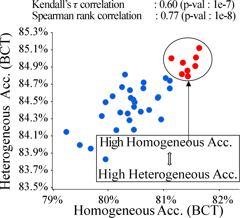
We plot the homogeneous accuracy of models with vanilla training (target of traditional NAS) \vsheterogeneous accuracy of the same models trained with BCT (our target) in Fig. 4(b). We observe that: (1) The correlation between the two accuracy is low and (2) The architectures with the highest heterogeneous accuracy are not those with highest homogeneous accuracy. This indicates traditional NAS may not be successful in searching for compatible architectures.

We further investigate the correlation between homogeneous (with BCT) and heterogeneous accuracy (with BCT) in Fig. 4(c) and discover that the correlation of these two accuracies is much higher than that in Fig. 4(b). This offers a key insight that equipping traditional NAS with BCT may help in searching compatible architectures.

Architecture optimization with Cmp-NAS Based on the intuition developed previously, we develop Cmp-NAS using the following notation. Denote by $\phi_{q}(a_{q},w_{q})$ a candidate query embedding model with architecture $a_{q}$ and weights $w_{q}$ . We further denote $\kappa_{q}$ as its corresponding classifier. With Cmp-NAS, we solve a two-step optimization problem where the first step amounts to learning the best set of weights— $w_{q}^{*}$ (for the embedding model $\phi_{q}$ ) and $\kappa_{q}^{*}$ (for the common classifier)–by minimizing a classification loss $\mathcal{L}$ over the training set $\mathcal{T}$ as below

w_{q}^{*},\kappa_{q}^{*}=\operatorname*{\arg\!\min}_{w_{q},\kappa_{q}}\{\lambda_{1}\mathcal{L}(\phi_{q}(a_{q},w_{q}),\kappa_{q};\mathcal{T})\\ +\lambda_{2}\mathcal{L}(\phi_{q}(a_{q},w_{q}),\kappa_{g};\mathcal{T})\},

(2)

where $\mathcal{L}$ can be any classification loss such as Cosine margin [wang2018cosface], Norm-Softmax [norm_softmax]. Similar to BCT, the second term $\mathcal{L}(\phi_{q}(a_{q},w_{q}),\kappa_{g};\mathcal{T})$ ensures that the candidate query embedding model $\phi_{q}(a_{q},w_{q}^{*})$ learns a representation that is compatible with the gallery classifier.

Using weights $w_{q}^{*}$ and $\kappa_{q}^{*}$ from above, the second step amounts to finding the best query architecture $a_{q}^{*}$ in a search space $\Omega$ , by maximizing a reward $\mathcal{R}$ evaluated on the validation set as below

a_{q}^{*}=\operatorname*{\arg\!\max}_{a_{q}\in\Omega}\mathcal{R}\left(\phi_{q}(a_{q},w_{q}^{*}),\kappa_{q}^{*}\right).

(3)

We consider three candidate rewards presented in Tab 1. Similar to traditional NAS, homogeneous accuracy $M(\phi_{q}(a_{q},w_{q}),\phi_{q}(a_{q},w_{q}))$ is our baseline reward $\mathcal{R}_{1}$ . Recall that however, we are interested in searching for the architecture which achieves the best heterogeneous accuracy. With this aim, we design rewards $\mathcal{R}_{2}$ and $\mathcal{R}_{3}$ which include the heterogeneous accuracy in their formulation.

Reward	Formulation
$\mathcal{R}_{1}$	$M(\phi_{q}(a_{q},w_{q}),\phi_{q}(a_{q},w_{q})$
$\mathcal{R}_{2}$	$M(\phi_{q}(a_{q},w_{q}),\phi_{g})$
$\mathcal{R}_{3}$	$M(\phi_{q}(a_{q},w_{q}),\phi_{q}(a_{q},w_{q}))\times M(\phi_{q}(a_{q},w_{q}),\phi_{g})$

Table 1: Different rewards considered with Cmp-NAS. The rewards

\mathcal{R}_{1}

\mathcal{R}_{2}

prioritize either the symmetric or asymmetric accuracy while ignoring the other.

\mathcal{R}_{3}

prioritizes both accuracies and consistently outperforms other rewards.

Our Cmp-NAS formulation in Eq. 2 and rewards in Tab. 1 is general and can work with any NAS method. For demonstration, we test our idea with the single path one shot NAS [NAS_SinglePath] and consists of the following two components:

Search Space: Similar to popular weight sharing methods [proxylessnas, NAS_SinglePath, DARTS], the search space of our query model consists of a shufflenet-based super-network. The super-network consists of $20$ sequentially stacked choice blocks. Each choice block can select one of four operations: $k\times k$ convolutional blocks ( $k\in{3,5,7}$ ) inspired by ShuffleNetV2 [ma2018shufflenet] and a $3\times 3$ Xception [chollet2017xception] inspired convolutional block. Additionally, each choice block can also select from 10 different channel choices $0.2-2.0\times$ . During training we use the loss formulation in Eq. 2 to train this super-network whereby, in each batch a new architecture is sampled uniformly [NAS_SinglePath] and only the weights corresponding to it are updated.

Search Strategy: To search for the most compatible architecture, Cmp-NAS uses evolutionary search [NAS_SinglePath] fitted with the different rewards outlined in Tab. 1. The search is fast because each architecture inherits the weights from the super-network. In the end, we obtain the five best architectures and re-train them from scratch with BCT.

4 Experiments

We evaluate the efficacy of our heterogeneous system on two tasks: face retrieval, as it is one of the “open-universe” problems with the largest publicly available datasets; and fashion retrieval which necessitates an open-set treatment due to the constant evolution of fashion items. We use face retrieval as the main benchmark for our ablation studies.

4.1 Datasets, Metrics and Gallery Model

Face Retrieval: We use the IMDB-Face dataset [IMDB] to train the embedding model for the face retrieval task. The IMDB-Face dataset contains over 1.7M images of about 59k celebrities. If not otherwise specified, we use $95\%$ of the data as training set to train our embedding model and use the remaining $5\%$ as a validation dataset to compute the rewards for architecture search. For testing, we use the widely used IJB-C face recognition benchmark dataset [IJBC]. The performance is evaluated using the true positive identification rate at a false positive identification rate of $10^{-1}$ (TPIR@FPIR= $10^{-1}$ ). Throughout the evaluation, we use a ResNet-101 as the fixed gallery model $\phi_{g}$ .

Fashion Retrieval: We evaluate the proposed method on Commercial-Consumer Clothes Retrieval task on DeepFashion2 dataset [Deepfashion2]. It contains 337K commercial-consumer clothes pairs in the training set, from which $90\%$ of the data is used for training the embedding and the rest $10\%$ is used for computing the rewards in architecture search. We report the test accuracy using Top-10 retrieval accuracy on the original validation set, which contains 10,844 consumer images with 12,377 query items, and 21,309 commercial images with 36,961 items in the gallery. ResNet-101 is used as the fixed gallery model $\phi_{g}$ .

4.2 Implementation Details

Our query and gallery models take a $112\times 112$ image as input and output an embedding vector of $128$ dimensions.

Face retrieval: We use mis-alignment and color distortion for data augmentation [shen2020towards]. Following recent state-of-the-art [wang2018cosface], we train our gallery ResNet-101 model using the cosine margin loss [wang2018cosface] with margin set to $0.4$ . We use the SGD optimizer with weight decay $5\times 10^{-4}$ . The initial learning rate is set to $0.1$ which decreases to $0.01$ , $0.001$ and $0.0001$ after $8$ , $12$ and $14$ epochs. Our gallery model is trained for $16$ epochs with a batch size $320$ . We train the query models for 32 epochs with a cosine learning rate decay schedule [Cosine_Annealing]. The initial learning rate is set to $1.3$ all query models except MobileNetV1( $1\times$ ) which uses $0.1$ .

Fashion retrieval: The original fashion retrieval task with DeepFashion2 [Deepfashion2] requires to first detect and then retrieve fashion items. Since we only tackle the retrieval task, we construct our retrieval-only dataset by using ground truth bounding box annotations to extract the fashion items. To train the gallery model, we follow [Zhai2019ClassificationIA] in using normalized cross entropy loss with temperature $0.5$ . The gallery model is trained for 40 epochs using an initial learning rate of $3.0$ with cosine decay. The weight decay is set to $10^{-4}$ . Our query models are trained with BCT for 80 epochs using an initial learning rate of $10$ with cosine decay.

Runtime: On a system containing 8 Tesla V100 GPUs, the entire pipeline for the face (and fashion) retrieval takes roughly 100 (45) hours. This includes roughly 8 (8) hours to train the gallery model, 32 (14) hours to train the query super-network, 48 (20) hours for evolutionary search and 2 (2) hours to train the final query architecture.

For additional implementation details specific to Cmp-NAS, please refer to the supplementary material.