Comparison of REML methods for the study of phenome-wide genetic variation
Abstract
It is now well documented that genetic covariance between functionally related traits leads to an uneven distribution of genetic variation across multivariate trait combinations, and possibly a large part of phenotype-space that is inaccessible to evolution. How the size of this nearly-null genetic space translates to the broader phenome level is unknown. High dimensional phenotype data to address these questions are now within reach, however, incorporating these data into genetic analyses remains a challenge. Multi-trait genetic analyses, of more than a handful of traits, are slow and often fail to converge when fit with REML. This makes it challenging to estimate the genetic covariance (G) underlying thousands of traits, let alone study its properties. We present a previously proposed REML algorithm that is feasible for high dimensional genetic studies in the specific setting of a balanced nested half-sib design, common of quantitative genetics. We show that it substantially outperforms other common approaches when the number of traits is large, and we use it to investigate the bias in estimated eigenvalues of G and the size of the nearly-null genetic subspace. We show that the high-dimensional biases observed are qualitatively similar to those substantiated by asymptotic approximation in a simpler setting of a sample covariance matrix based on i.i.d. vector observation, and that interpreting the estimated size of the nearly-null genetic subspace requires considerable caution in high-dimensional studies of genetic variation. Our results provide the foundation for future research characterizing the asymptotic approximation of estimated genetic eigenvalues, and a statistical null distribution for phenome-wide studies of genetic variation.
1 Introduction
To answer the most compelling questions in evolutionary biology we must uncover the causal connection between genotypes, phenotypes, and the environment (selection). Unlike the finite genomes that underlie them, organisms are comprised of essentially infinite phenotypes that may genetically vary and covary. While not all of those phenotypes will be meaningful for fitness, there are at least many thousands to consider, if we are to begin to understand the genotype-phenotype map. Efforts to increase the scope and throughput of phenotyping have been cited as an urgent priority in evolutionary biology since at least 2010 (Houle, 2010; Houle et al., 2010). High-throughput phenomic technologies such as such as RNA sequencing (Schrag et al., 2018), drone based plant imaging (Furbank and Tester, 2011), wearable sensors (Haleem et al., 2021; Sharma et al., 2021; Neethirajan, 2017), metabolomics for physiological measurements (Jin et al., 2020; Freimer and Sabatti, 2003), and computer vision for morphometrics (Lürig et al., 2021) are now within reach. However, incorporating these high-dimensional phenotype data into genetic analyses remains a challenge.
Multivariate studies of genetic variation focusing on relatively small sets of traits (small p) have transformed our understanding of how genetic variation is distributed across phenotypes, and how this affects evolutionary outcomes. While almost all individual traits studied have been shown to have genetic variation (Lynch et al., 1998), and responses to artificial selection are often rapid and of large magnitude (Hill and Kirkpatrick, 2010), multivariate studies of the genetic variance-covariance matrix (G) show that this genetic variation is distributed unevenly across multivariate phenotypes (Kirkpatrick, 2009; Sztepanacz and Houle, 2019). The concentration of genetic variance onto fewer multivariate trait combinations than the number of phenotypes measured is biologically caused by the pleiotropic effects of alleles on multiple traits which leads to their genetic covariance (Lande, 1980). Multivariate trait combinations with high genetic variation form a genetic subspace where traits are predicted to have high evolvability. Evolution is predicted to occur more quickly along these multivariate trait combinations than in any individual trait (Agrawal and Stinchcombe, 2009), contributing to divergence among populations (eg. (McGlothlin et al., 2022; Schluter, 1996)), species (eg. (Innocenti and Chenoweth, 2013; Bégin and Roff, 2004)), and sexes (eg. Gosden and Chenoweth (2014)). The set of orthogonal multivariate trait combinations with low genetic variation, form a complementary subspace which is termed the nearly-null genetic subspace (Gomulkiewicz and Houle, 2009; Gaydos et al., 2013). This subspace putatively represents important evolutionary constraints in natural populations, where phenotypic evolution is expected to be constrained (Gomulkiewicz and Houle, 2009), occur slowly (Kirkpatrick, 2009) or stochastically (Hine et al., 2014).
Estimating the size of the nearly-null genetic subspace is an avenue to quantify both genetic constraints that may lead to evolutionary limits, and the extent of pleiotropy underlying organisms, which determines their genetic dimensionality. Past studies have typically found that genetic variance is restricted to less than half of the phenotype space with most multivariate trait combinations having no detectable genetic variation (Blows and McGuigan, 2015) . One notable exception to this pattern is Drosophila wing shape, which as been shown to have genetic variation in all multivariate wing shape traits (ie. a full rank G) (Mezey and Houle, 2005; Sztepanacz and Blows, 2015; Sztepanacz and Houle, 2019; Houle and Meyer, 2015). These multivariate studies have typically dealt with small sets of functionally related traits such as wing (Mezey and Houle, 2005), skeletal (Garcia et al., 2014) or phyto (Walsh and Lynch, 2018) morphology, or traits that have a strong physiological (Caruso et al., 2005), or biochemical relationships (Sztepanacz and Rundle, 2012). Therefore, genetic covariance among these traits may be relatively high compared to the range of traits that are possible to study with phenomics. Whether inferences for the size of the nearly null subspaces found in these small p studies can be extrapolated to phenomes is an open biological question.
Confounded with the biological phenomena that nearly-null genetic subspaces represent, are the statistical phenomena that arise from their estimation. Even in low p studies, estimating G and its eigenvalues is a challenge. The standard approach is to fit a multivariate mixed model in REML to estimate G as an unstructured covariance matrix. These models commonly fail to converge with only a small number of traits, and run-times are long because of the quadratic growth in the number of parameters to estimate with the number of traits. As shown in the one-way MANOVA context, small p models that do converge, often produce estimated matrices that are not positive definite (Hill and Thompson, 1978) and that have overdispersed eigenvalues (Hayes and Hill, 1981), properties which are exacerbated in the two-way hierarchical model, such as the nested half-sib design common in quantitative genetic studies. In particular, Hayes and Hill (1981) show that the magnitude of overdisperion of the genetic eigenvalues is determined by with smaller sample sizes or more traits leading to larger dispersion. The overdispersion of estimated eigenvalues is a pattern remarkably similar to that we interpret biologically as genetic subspaces of high evolvability and those that are nearly null. In the phenomic context, where or possibly even greater than 1, it could even obscure any biological signal. Disentangling how much of the dispersion of eigenvalues of G is due to biological covariance versus statistical estimation is therefore important, if we want to predict evolutionary constraints.
In simpler settings, recent work has provided a quantitative description of the bias and error related to the dispersion of estimated eigenvalues when is of order comparable to , summarized for example in (Johnstone and Paul, 2018). The bulk eigenvalue distribution of sample (i.i.d) covariance matrices, such as those describing among-individual covariance structure such as phenotypic covariance matrices P, or genomic relatedness matrices (GRMs), is known to follow the Marchenko Pastur distribution (Marčenko and Pastur, 1967; Yao et al., 2015). For a large class of mixed models, including full-sib and half-sib designs, and for the particular case of MANOVA estimators, overdisperson of sample eigenvalues in the bulk eigenvalue distribution is described by a generalization of the Marchenko-Pastur distribution (Fan and Johnstone, 2019).
The individual eigenvalues of sample covariance matrices also follow particular distributions. The leading eigenvalue conforms to the Tracy-Widom distribution, both for sample (i.i.d.) covariance matrices (Johnstone, 2001) and for MANOVA estimates from mixed models(Fan and Johnstone, 2022). The trailing (smallest) eigenvalue converges to a reflected Tracy-Widom distribution (Fan and Johnstone, 2022). Again for MANOVA estimates in mixed models, the leading estimated eigenvalues and eigenvectors can be influenced by an alignment between directions of sufficiently elevated variance in the different covariance components (Fan et al., 2018). For example, an alignment between the major axis of genetic variance and environmental variation could lead to an estimated that is biased toward the major axis of environmental variation and with an eigenvalue that is much larger than it should be. These quantitative descriptions provide appropriate null distributions for MANOVA eigenvalues, and enable bias-correction for estimated eigenvalues in these contexts.
Simple among line (one-way) genetic simulation studies estimating G for p=5 using REML, combined with an empirical centering and scaling approach (Saccenti et al., 2011), suggest that REML eigenvalues may have similar properties. The bulk distribution of eigenvalues appears to follow the Marchenko Pastur distribution (Blows and McGuigan, 2015), and the leading eigenvalues of estimated G are consistent with the Tracy Widom distribution (Sztepanacz and Blows, 2017). Notably, however, the leading eigenvalues of G estimated using factor analysis or MCMCglmm do not follow the Tracy Widom distribution (Sztepanacz and Blows, 2017), showing that the method used to estimate G influences the sampling distribution of its eigenvalues. These studies laid the groundwork for determining the properties of REML eigenvalues in the one-way design, however, they are limited to small p and . A major hurdle in extrapolating these studies to the phenomic-scale, is the difficulty in employing REML for high p.
Alternative approaches to REML have been developed in recent years and employed to estimate G and its eigenvalues for high p phenomic studies. The Bayesian sparse factor approach of Runcie and Mukherjee (2013) enables the estimation of genetic covariance for thousands of traits by placing a prior on the latent factors underlying G and E that few traits contribute to them (ie. they are sparse). Studies using this method have qualitatively found the same uneven distribution of standing genetic variation (Garcia et al., 2014), mutational variation (Hine et al., 2018), and a large nearly-null genetic subspace, as seen in small p studies. While biologically motivated, the assumption that sparse factors underlie both G and E may upwardly bias estimates of the nearly null subspace. MegaLMM (Runcie et al., 2021) uses strong Bayesian priors on the sparsity and number of important latent factors underlying G and E to fit linear mixed models for traits and relatively small n. The primary goal of this approach, however, is for genomic prediction, not estimation. Consequently, the properties that make the method feasible for including phenome-level data, and which are beneficial for genomic prediction, may have undesirable properties with respect to estimation. Blows et al. (2015) circumvented convergence problems in REML by constructing large G from a set of overlapping principal sub-matrices, estimated for a small numbers of traits using REML. Since the constructed matrix is not guaranteed to be positive definite, a subsequent bending (Hayes and Hill, 1981; Meyer, 2019) of G was required. This approach enabled a coarse description of the distribution of genetic variation across G, finding that the vast majority of genetic variation was found in few dimensions. However, a quantitative description of the size of the nearly null subspace was not possible. While each of these approaches have value in certain circumstances, they all make some undesirable assumptions that lead to challenges in interpreting the size of the nearly null space and performing statistical hypothesis testing.
In this paper we demonstrate that REML is feasible for high p phenomics in the specific setting of a balanced nested half-sib design, without having to make any additional assumptions about the structure of G or perform any bending, and we begin to study the properties of estimated eigenvalues from these high p models. In particular, we perform simulation study investigating the spectral characteristics of the REML estimate of for a family of balanced half-sib breeding designs in the moderate- () setting.
As algorithms that are usually used to fit mixed models often fail to converge even for as small as , we use an algorithm designed specifically for fitting balanced nested designs introduced in Calvin and Dykstra (1991) that will allow us to find REML estimates for larger values of .
In section 3, we compare this Calvin-Dijkstra algorithm with various other procedures used to compute or approximate the REML estimate, showing that it does at least as well as its common alternatives. We then demonstrate that the algorithm is a practical method for REML estimation for the balanced designs even for , in which regard it substantially outperforms the alternatives presented.
Sections 4 and 5 investigate the illustrate the biases inherent in using functions of eigenvalues of the REML estimate to estimate the corresponding functions of the eigenvalues of . We show that, as gets large, the large eigenvalues of have a substantial upward bias when used to estimate the large eigenvalues of . We also investigate the bias in estimators of the nearly-null dimension of based on counting small eigenvalues of . These biases are more difficult to describe, so we demonstrate the behavior of such estimators on a family of qualitatively different between-sire and between-dam covariance matrices. Section 6 has some summary conclusions and discussion.
2 Description of methods compared
Our simulations use a balanced half-sib (or nested two-way) design
| (1) |
Here and are the random effects due to sire, dam and individual respectively, and is a fixed intercept.
Each is a vector of traits; there are and possible values of the indices and . Each random effect vector is assumed to follow independent normal distributions
| (2) |
We are particularly interested in estimation of the genetic covariance matrix and its eigenvalues, but will also look at the concomitant estimates of and . The estimates we will compare are
-
•
MANOVA, which are easy to compute but do not necessarily produce a positive-definite estimate for ,
-
•
REML-lme. fitted using a generic mixed-effects model solver (we use R function lme()), which should converge to the true REML estimates but are prohibitively slow to compute for high (or even moderate) numbers of traits,
-
•
pseudo-REML, as described by Amemiya (1985). These are easy to compute, and in the full-sub (one-way) design are exactly the REML estimates. In the half-sib case, they are only approximations.
-
•
stepwise REML, as described by Calvin and Dykstra (1991) This is an iterative algorithm that converges to the true REML estimates. Although we know of no results decribing the rate of convergence, in practice it is very fast, allowing for easy REML estimation even for matrices.
-
•
pairwise REML, in which the estimates of the individual entries are computed using a bivariate analysis with traits and . This estimate is sometimes proposed as a computational fall-back when the dimensionality of is too high for REML to converge; it need not be non-negative definite, as will be seen.
3 Initial examples
3.1 A small example with zero eigenvalues
As a warm-up, we first illustrate the methods in a setting with a small number of traits, .111indeed, this was the largest number of traits for which lme() runs relatively quickly. Specifically, we take
| (3) |
and diagonal structures for the variance component matrices:
| (4) | ||||||
This information is not used when fitting – all procedures are run with no assumptions on the covariances. The vector , but its value is immaterial to all methods used here.
All simulations were done in R; the software and technical descriptions of code used to produce the results of this paper are available in an R package hosted at https://github.com/damian-t-p/REMLSimulationPaper.
Table 1 shows the results of one sample realization, about which the following remarks may be made.
-
•
For MANOVA, as expected, the zero eigenvalues of lead to some negative estimated eigenvalues. The REML criterion is higher than that of the actual REML estimate found by stepwise REML. This is because MANOVA in this balanced setting in fact maximizes the likelihood over a larger set, i.e. without enforcing the non-negativity constraints.
-
•
the Calvin-Dykstra (CD) algorithm for stepwise-REML exhibited linear convergence in the REML criterion (not shown here). The CD convergence criterion uses
where is the vector of covariance estimates after the th iteration. We stopped when .
-
•
The pseudo REML estimates are close, but not identical, to the stepwise REML ones, and the REML criterion score is lower.
-
•
REML-lme is slow and often fails to converge: we record the results at termination, even before convergence, and for this reason the REML criterion score is less than that of stepwise REML, which does converge to the maximum.
3.2 An example with
An important advantage of stepwise REML is that it is can easily be run for relatively large numbers of traits. In this section, we use , but can be in the thousands before the stepwise REML estimate takes more than a second to compute.
The parameters are as in (3)– (3.1), but with some modifications:
| (5) |
where are all independent standard normal deviates.
Figure 1 compares the eigenvalues of (in blue) next to the true eigenvalues of (in red). Now that is of the same order as , the sample eigenvalues are much more spread out than those of – we see that the REML estimate zeroes out many eigenvalues while overestimating a few others.

3.3 Pairwise REML with
We investigate the strategy of computing pairwise REML estimates for each pair of traits. We create a new estimate such that the diagonal entries are computed by doing a single-trait analysis on trait and the off-diagonal entries are computed by doing a 2-trait analysis on the traits .
The setting is the same as the previous subsection, especially (5). In fact, we used the stepwise-REML estimates for the 2-trait analyses, since there are 1250 entries of to fill in, and even in the 2-dimensional case, fitting a generic mixed model is too slow for this. However, we can still compare the resulting with the REML esimate to see how the eigenvalues produced by the pairwise procedure differ from those done by computing the whole stepwise REML estimate at once.

Let be the eigenvalues of and be the eigenvalues of . Figure 2 plots the differences against . We may observe that
-
•
the pairwise REML estimate is not positive definite: some of its estimated eigenvalues lie between and ,
-
•
the pairwise REML eigenvalues are all smaller than the actual REML ones: for all ,
-
•
when the pairwise REML eigenvalues are positive, the differences are not large: an empirical summary (in this case) might be that typically,
4 Repeated sampling
The Calvin-Dykstra algorithm is fast enough that it is possible to study the properties of REML estimates of eigenvalues through simulation.
4.1 Bias in top eigenvalues
This example confirms the upward bias in the largest eigenvalues of the REML estimates and confirms that the bias increases with the number of traits .
Again we use the half-sib design (1)– (2) with and
| (6) |
The number of traits grows from 10 to 100 in increments of 10. Over replications, the averages of the top 5 eigenvalues of and are plotted against . Also shown (thick red lines) are the corresponding population eigenvalues ( and respectively).

Some remarks on the results in Figure 3:
-
•
the means are biased upwards, as expected, but the biases are much more substantial for (especially) and than for . Also notable is the rapid increase in the biases with in each case,
-
•
The standard deviations of the 50 replicates were computed for each eigenvalue (results not shown here). These were markedly larger for and (between 0.2 and ) than for (between 0.02 and 0.03). Although obscured by sample fluctuation, it appears — as might be expected — that the SDs are ordered, decreasing as we move down from the top eigenvalue to the 5th. There is no clear dependence on in the SDs.
-
•
In this setting the REML estimates coincide with the MANOVA estimators. This is because all of the population eigenvalues of and in (6) are well separated from , and the MANOVA estimates were in all cases positive definite.
4.2 Differences between the largest REML and MANOVA eigenvalues
In contrast to the previous example, when nearly null genetic subspaces are present we expect the REML estimates to differ significantly from MANOVA as the smallest MANOVA eigenvalues will be negative. Here we examine the difference between the largest eigenvalues and for REML and MANOVA for .
We set half of the diagonal entries of and to zero at random, leaving and all other parameters unchanged from the previous subsection. Figure 4 shows the mean differences (averaged over 50 replications) of as a function of . We observe that
-
•
the mean differences again increase in absolute value, nearly linearly, as increases,
-
•
for the top REML eigenvalues are larger than MANOVA, while for and they are smaller,
-
•
the magnitude of the (negative) difference is much larger for ,
-
•
the SDs of the differences over the 50 replications (not shown) are approximately 10% of the mean differences, and in particular are generally increasing with .
These variations in sign and magnitude of the differences between the top REML and MANOVA eigenvalues call for further study. At the least they indicate a dependence on the level of nesting of the respective variance components.

5 Nearly Null Subspaces
5.1 Counting zero eigenvalues in REML estimator
In this section we simulate several half-sib designs in which has null spaces of various dimensions . We might expect the number of zero (or small) eigenvalues of the corresponding REML estimates to track the null space dimension . We will see that this is broadly true, but that again significant biases are present.
Specification of – generalities. In general, the principal axes of variation (i.e. eigenvectors) of the covariance matrices need not be aligned, and so to use only diagonal matrices in our investigations would entail a loss of generality.
We will therefore allow for examples of non-alignment of the axes of and , but for simplicity we keep the error covariance scalar: . Because the model (1)— (2) is Gaussian, the REML and MANOVA estimates are unchanged by rotation (an orthogonal transformation) of the data. This means that we can take to be diagonal (and is unchanged), but that need not be.
Specifically suppose that has eigendecomposition for suitable orthogonal and diagonal matrices and respectively. Then the REML estimates are the same for the model with parameters as for the model with parameters .
In summary, the following are important to note: {Itemize}
We can only assume a diagonal structure for one of or , but not both,
If we are interested in estimating something about other than the eigenvalues, we cannot assume a diagonal structure for ,
If we do not assume that is a scalar matrix, then it cannot be assumed to be diagonal either.
Settings for : Thus, we will consider the following specifications for :
| (7) |
with the choices
A typical draw from each of these cases (with zeros) might be summarized qualitatively as follows:
-
•
Identity: 40 non-zero eigenvalues all equal to 1,
-
•
Chi-squared: 40 nonzero eigenvalues spread unevenly over the range ,
-
•
Heavy-tailed: 39 nonzero eigenvalues spread unevenly over with an outlier (e.g. at 750).
Settings for : We consider one scalar and three non-diagonal cases:
| (8) |
In a little more detail:
-
•
Identity: sets all 50 eigenvalues equal to 1,
-
•
Wishart: Let be a matrix of iid random variables. Then we form , which is the sample covariance of . Since the population covariance of the columns of is , is not too far from , while still having uniformly distributed eigenvectors. The eigenvalues of are unevenly spread between 0 and 4222and are approximately a sample from a Marcenko-Pastur quarter circle law with parameter .
-
•
High-rank: Let be a matrix of orthonormal vectors drawn uniformly. Let be diagonal matrix with iid entries on the diagonal. We then take . This matrix has eigenvectors independent from those of , but the eigenvalues are more spread out than those in the Wishart case.
-
•
High-corr: is a square matrix with s on the diagonal and s in every other entry. This can be represented as , where is a vector of ones. This means that the eigenvalues of are with multiplicity and with multiplicity .
Remaining parameter settings: In all cases, the error covariance is taken to be the identity . We use the following set parameter values:
-
•
Number of traits, ,
-
•
Number of sires, dams per sire, and individuals per dam: ,
-
•
Number of repetitions, .
Moreover, the following variables:
-
•
Dimensions of null space ,
-
•
Additional sire covariance scaling .
Results: For each combination of and structures and the null space dimension and scaling variables and described above, we compute the eigenvalues of the REML estimate of .
Let be the number of eigenvalues of that are exactly zero. Figure 5 plots (vertical axis) against , the ‘true’ null space dimension. The solid line and ribbon show the mean and interquartile range computed from the replicates. As a reference, the line is shown on each plot with black dashes.
In all cases, the estimated nearly-null dimension tends to be moderated: when is large, is an underestimate, and vice-versa when is small. Moreover, it seems that the structure of that is the main factor governing the shape of the curve.
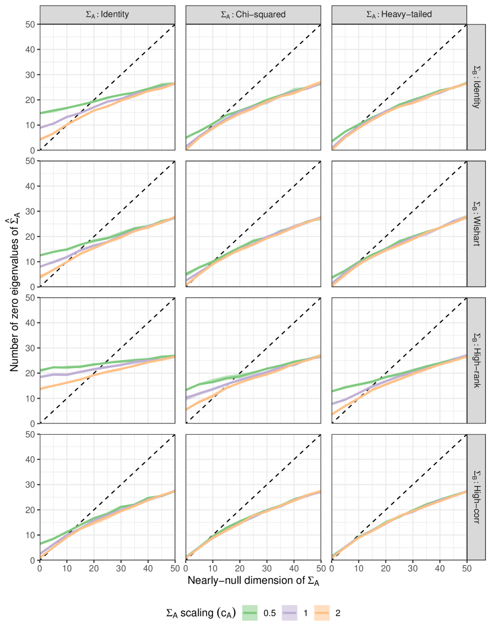
We can perform similar analyses with different estimators of . Consider, for example
Figure 6 has the same features as fig. 5, but instead displays the number of “small” eigenvalues of , defined here as the number of eigenvalues with a value below , i.e. .
This always exceeds the number of eigenvalues of that are exactly zero, and so, as we might expect, it improves the under-estimates at the expense of the over-estimates.
This estimator does particularly well when has well-separated eigenvalues - that is in the high-correlation and identity cases and when the eigenvalues of are larger (chi-squared and heavy-tailed cases).

5.2 Bias in
Again we allow the dimension of the null space of to vary, but now turn attention to biases in the REML estimate of the largest eigenvalue.
The previous simulation setting is used, except that the following structures are used for :
| (9) |
(*): the variates are held the same across replications to reduce variation.
We focus on the top eigenvalue of the MANOVA and REML estimates of the sire covariance , namely and respectively across the settings, with replications. Figure 7 shows the behavior of the relative differences .
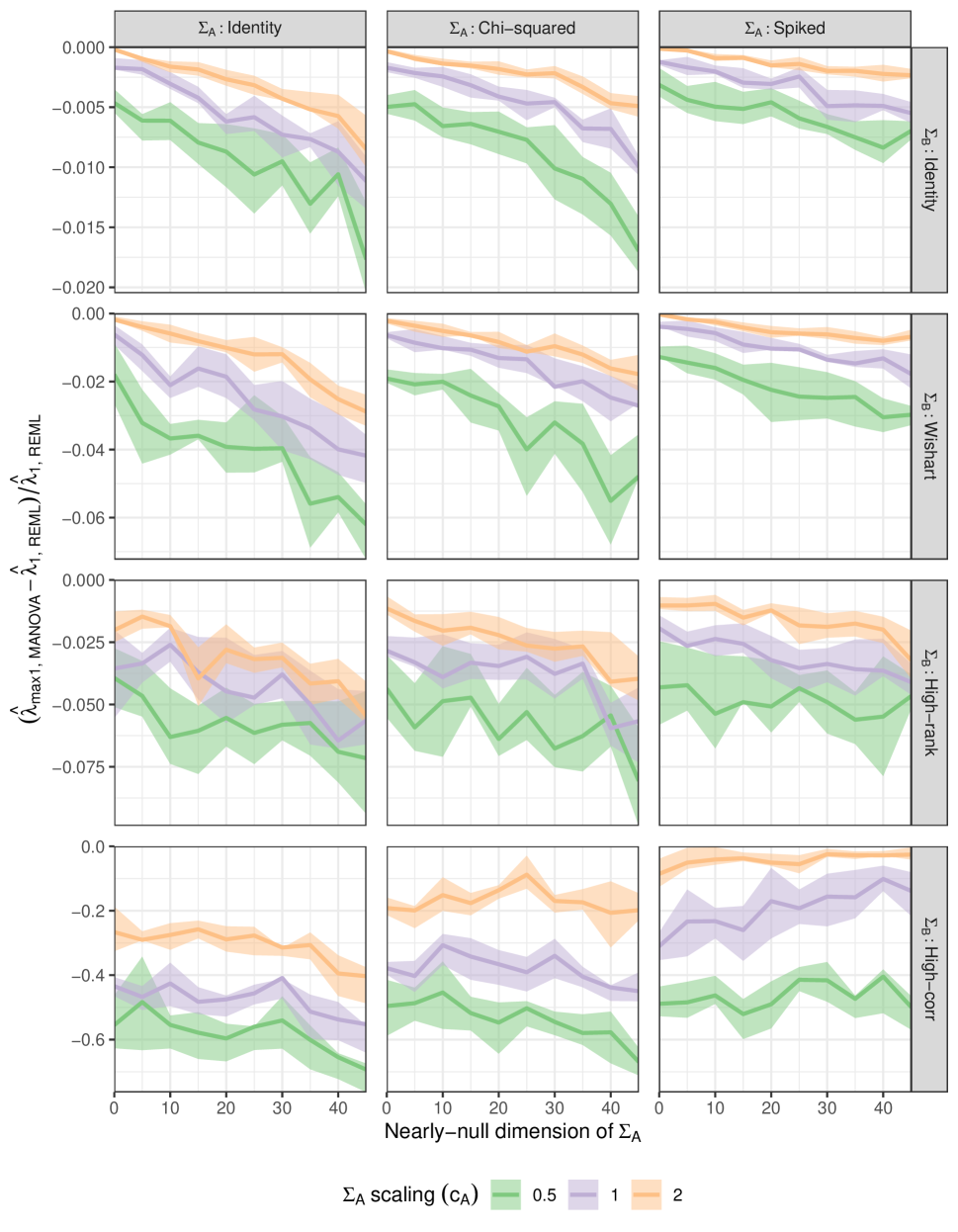
-
•
Empirically, it always happens that ,
-
•
The size of the relative differences depends strongly on , being much larger for ‘highcorr’ (which has a single large spike eigenvalue) than for the other cases, where the difference is smaller, but not insignificant,
-
•
the relative differences also tend to increase in magnitude with the null space dimension .
-
•
the relative differences also tend to vary inversely with the sire variance scaling .
We can also investigate the bias in by plotting the relative difference where is the largest eigenvalue of the true underlying covariance matrix , Figure 8.

We may make the following remarks about the upward bias of the REML estimate relative to the truth:
-
•
it depends on the structure, rank and magnitude of both and
-
•
it is particularly large when the nonzero eigenvalues of are all the same (‘identity’), though in this case the eigenvalues of are smaller than for ‘chisquared’ and ‘spiked’,
-
•
it is smallest in the high correlation case .
6 Discussion
We have shown that the Calvin-Dykstra convex duality algorithm renders REML feasible for high- phenomics in the very specific setting of balanced half-sib designs.333Calvin (1993) proposed an extension of the Calvin-Dykstra algorithm to unbalanced half-sib designs, using the EM algorithm to impute missing observations. In current work we are implementing this algorithm in order to apply it to some publicly available datasets that are beyond current capabilities of more generic REML solvers.
While the balanced observation assumption in this paper is unrealistic in practice, it does allow initial demonstration of statistical estimation phenomena for larqe that will likely carry over to unbalanced settings and more complex designs. We have seen examples of two such phenomena in the simulations conducted here.
First there are significant biases in estimating the dimension of a null space in the genetic covariance by simply counting the number of zero REML eigenvalues: it is typically biased high when is small and biased low when is large. Second, there are significant biases of overestimation in the REML estimates of the largest eigenvalues of genetic covariance matrices.
Both these high dimensional biases are not unexpected if one recalls similar phenomena (eigenvalue spreading and biases) that have been observed and substantiated by asymptotic approximation in two simpler settings: estimation of a single -dimensional covariance matrix based on i.i.d. vector observations (reviewed in Johnstone and Paul (2018)), and MANOVA estimates in the present high dimensional variance component models (Fan and Johnstone, 2019, 2022; Fan et al., 2018). It is a natural topic for future research to look for greater understanding of REML in high- settings, for example via asymptotic approximations.
In summary, the simulations in this work, even with their limitation to specific settings in special balanced designs, already indicate that considerable caution will be needed in interpreting REML estimates in phenome-wide studies of genetic variation.
References
- Agrawal and Stinchcombe [2009] Aneil F Agrawal and John R Stinchcombe. How much do genetic covariances alter the rate of adaptation? Proceedings of the Royal Society B: Biological Sciences, 276(1659):1183–1191, March 2009. ISSN 0962-8452, 1471-2954. doi: 10.1098/rspb.2008.1671. URL https://royalsocietypublishing.org/doi/10.1098/rspb.2008.1671.
- Amemiya [1985] Yasuo Amemiya. What should be done when an estimated between-group covariance matrix is not nonnegative definite? The American Statistician, 39(2):112–117, 1985.
- Blows and McGuigan [2015] Mark W. Blows and Katrina McGuigan. The distribution of genetic variance across phenotypic space and the response to selection. Molecular Ecology, 24(9):2056–2072, May 2015. ISSN 09621083. doi: 10.1111/mec.13023. URL https://onlinelibrary.wiley.com/doi/10.1111/mec.13023.
- Blows et al. [2015] Mark W. Blows, Scott L. Allen, Julie M. Collet, Stephen F. Chenoweth, and Katrina McGuigan. The Phenome-Wide Distribution of Genetic Variance. The American Naturalist, 186(1):15–30, July 2015. ISSN 0003-0147, 1537-5323. doi: 10.1086/681645. URL https://www.journals.uchicago.edu/doi/10.1086/681645.
- Bégin and Roff [2004] Mattieu Bégin and Derek A. Roff. From micro- to macroevolution through quantitative genetic variation: positive evidence from field crickets. Evolution, 58(10):2287–2304, October 2004. ISSN 0014-3820, 1558-5646. doi: 10.1111/j.0014-3820.2004.tb01604.x. URL https://onlinelibrary.wiley.com/doi/10.1111/j.0014-3820.2004.tb01604.x.
- Calvin [1993] James A. Calvin. REML estimation in unbalanced multivariate variance components models using an em algorithm. Biometrics, 49(3):691–701, 1993. ISSN 0006341X, 15410420. URL http://www.jstor.org/stable/2532190.
- Calvin and Dykstra [1991] James A. Calvin and Richard L. Dykstra. Maximum likelihood estimation of a set of covariance matrices under Löwner order restrictions with applications to balanced multivariate variance components models. Ann. Statist., 19(2):850–869, 1991.
- Caruso et al. [2005] Christina M. Caruso, Hafiz Maherali, Alison Mikulyuk, Kjarstin Carlson, and Robert B. Jackson. Genetic variance and covariance for physiological traits in lobelia:are there constraints on adaptive evolution? Evolution, 59(4):826–837, April 2005. ISSN 0014-3820, 1558-5646. doi: 10.1111/j.0014-3820.2005.tb01756.x. URL https://onlinelibrary.wiley.com/doi/10.1111/j.0014-3820.2005.tb01756.x.
- Fan and Johnstone [2019] Zhou Fan and Iain M. Johnstone. Eigenvalue distributions of variance components estimators in high-dimensional random effects models. The Annals of Statistics, 47(5), October 2019. ISSN 0090-5364. doi: 10.1214/18-AOS1767. URL https://projecteuclid.org/journals/annals-of-statistics/volume-47/issue-5/Eigenvalue-distributions-of-variance-components-estimators-in-high-dimensional-random/10.1214/18-AOS1767.full.
- Fan and Johnstone [2022] Zhou Fan and Iain M. Johnstone. Tracy–Widom at each edge of real covariance and MANOVA estimators. The Annals of Applied Probability, 32(4):2967 – 3003, 2022. doi: 10.1214/21-AAP1754. URL https://doi.org/10.1214/21-AAP1754.
- Fan et al. [2018] Zhou Fan, Iain M. Johnstone, and Yi Sun. Spiked covariances and principal components analysis in high-dimensional random effects models, June 2018. URL http://arxiv.org/abs/1806.09529. arXiv:1806.09529 [math, stat].
- Freimer and Sabatti [2003] Nelson Freimer and Chiara Sabatti. The Human Phenome Project. Nature Genetics, 34(1):15–21, May 2003. ISSN 1061-4036, 1546-1718. doi: 10.1038/ng0503-15. URL http://www.nature.com/articles/ng0503-15.
- Furbank and Tester [2011] Robert T Furbank and Mark Tester. Phenomics–technologies to relieve the phenotyping bottleneck. Trends in plant science, 16(12):635–644, 2011. Publisher: Elsevier.
- Garcia et al. [2014] Guilherme Garcia, Erika Hingst-Zaher, Rui Cerqueira, and Gabriel Marroig. Quantitative Genetics and Modularity in Cranial and Mandibular Morphology of Calomys expulsus. Evolutionary Biology, 41(4):619–636, December 2014. ISSN 0071-3260, 1934-2845. doi: 10.1007/s11692-014-9293-4. URL http://link.springer.com/10.1007/s11692-014-9293-4.
- Gaydos et al. [2013] Travis L. Gaydos, Nancy E. Heckman, Mark Kirkpatrick, J. R. Stinchcombe, Johanna Schmitt, Joel Kingsolver, and J. S. Marron. Visualizing genetic constraints. The Annals of Applied Statistics, 7(2), June 2013. ISSN 1932-6157. doi: 10.1214/12-AOAS603. URL https://projecteuclid.org/journals/annals-of-applied-statistics/volume-7/issue-2/Visualizing-genetic-constraints/10.1214/12-AOAS603.full.
- Gomulkiewicz and Houle [2009] Richard Gomulkiewicz and David Houle. Demographic and Genetic Constraints on Evolution. The American Naturalist, 174(6):E218–E229, December 2009. ISSN 0003-0147, 1537-5323. doi: 10.1086/645086. URL https://www.journals.uchicago.edu/doi/10.1086/645086.
- Gosden and Chenoweth [2014] Thomas P. Gosden and Stephen F. Chenoweth. The evolutionary stability of cross-sex, cross-trait genetic covariances: evolutionary stability of cross-sex, cross-trait genetic covariances. Evolution, 68(6):1687–1697, June 2014. ISSN 00143820. doi: 10.1111/evo.12398. URL https://onlinelibrary.wiley.com/doi/10.1111/evo.12398.
- Haleem et al. [2021] Abid Haleem, Mohd Javaid, Ravi Pratap Singh, Rajiv Suman, and Shanay Rab. Biosensors applications in medical field: A brief review. Sensors International, 2:100100, 2021. ISSN 26663511. doi: 10.1016/j.sintl.2021.100100. URL https://linkinghub.elsevier.com/retrieve/pii/S2666351121000218.
- Hayes and Hill [1981] J. F. Hayes and W. G. Hill. Modification of Estimates of Parameters in the Construction of Genetic Selection Indices (’Bending’). Biometrics, 37(3):483, September 1981. ISSN 0006341X. doi: 10.2307/2530561. URL https://www.jstor.org/stable/2530561?origin=crossref.
- Hill and Thompson [1978] W. G. Hill and R. Thompson. Probabilities of Non-Positive Definite between-Group or Genetic Covariance Matrices. Biometrics, 34(3):429, September 1978. ISSN 0006341X. doi: 10.2307/2530605. URL https://www.jstor.org/stable/2530605?origin=crossref.
- Hill and Kirkpatrick [2010] William G. Hill and Mark Kirkpatrick. What Animal Breeding Has Taught Us about Evolution. Annual Review of Ecology, Evolution, and Systematics, 41(1):1–19, December 2010. ISSN 1543-592X, 1545-2069. doi: 10.1146/annurev-ecolsys-102209-144728. URL https://www.annualreviews.org/doi/10.1146/annurev-ecolsys-102209-144728.
- Hine et al. [2014] Emma Hine, Katrina McGuigan, and Mark W. Blows. Evolutionary Constraints in High-Dimensional Trait Sets. The American Naturalist, 184(1):119–131, July 2014. ISSN 0003-0147, 1537-5323. doi: 10.1086/676504. URL https://www.journals.uchicago.edu/doi/10.1086/676504.
- Hine et al. [2018] Emma Hine, Daniel E Runcie, Katrina McGuigan, and Mark W Blows. Uneven Distribution of Mutational Variance Across the Transcriptome of Drosophila serrata Revealed by High-Dimensional Analysis of Gene Expression. Genetics, 209(4):1319–1328, August 2018. ISSN 1943-2631. doi: 10.1534/genetics.118.300757. URL https://academic.oup.com/genetics/article/209/4/1319/5931002.
- Houle and Meyer [2015] D. Houle and K. Meyer. Estimating sampling error of evolutionary statistics based on genetic covariance matrices using maximum likelihood. Journal of Evolutionary Biology, 28(8):1542–1549, August 2015. ISSN 1010-061X, 1420-9101. doi: 10.1111/jeb.12674. URL https://onlinelibrary.wiley.com/doi/10.1111/jeb.12674.
- Houle [2010] David Houle. Numbering the hairs on our heads: The shared challenge and promise of phenomics. Proceedings of the National Academy of Sciences, 107(suppl_1):1793–1799, January 2010. ISSN 0027-8424, 1091-6490. doi: 10.1073/pnas.0906195106. URL https://pnas.org/doi/full/10.1073/pnas.0906195106.
- Houle et al. [2010] David Houle, Diddahally R. Govindaraju, and Stig Omholt. Phenomics: the next challenge. Nature Reviews Genetics, 11(12):855–866, December 2010. ISSN 1471-0056, 1471-0064. doi: 10.1038/nrg2897. URL http://www.nature.com/articles/nrg2897.
- Innocenti and Chenoweth [2013] Paolo Innocenti and Stephen F. Chenoweth. Interspecific Divergence of Transcription Networks along Lines of Genetic Variance in Drosophila: Dimensionality, Evolvability, and Constraint. Molecular Biology and Evolution, 30(6):1358–1367, June 2013. ISSN 1537-1719, 0737-4038. doi: 10.1093/molbev/mst047. URL https://academic.oup.com/mbe/article-lookup/doi/10.1093/molbev/mst047.
- Jin et al. [2020] Kelly Jin, Kenneth A. Wilson, Jennifer N. Beck, Christopher S. Nelson, George W. Brownridge, Benjamin R. Harrison, Danijel Djukovic, Daniel Raftery, Rachel B. Brem, Shiqing Yu, Mathias Drton, Ali Shojaie, Pankaj Kapahi, and Daniel Promislow. Genetic and metabolomic architecture of variation in diet restriction-mediated lifespan extension in Drosophila. PLOS Genetics, 16(7):e1008835, July 2020. ISSN 1553-7404. doi: 10.1371/journal.pgen.1008835. URL https://dx.plos.org/10.1371/journal.pgen.1008835.
- Johnstone and Paul [2018] I. M. Johnstone and D. Paul. PCA in high dimensions: An orientation. Proceedings of the IEEE, 106(8):1277–1292, Aug 2018. ISSN 0018-9219. doi: 10.1109/JPROC.2018.2846730.
- Johnstone [2001] Iain M. Johnstone. On the distribution of the largest eigenvalue in principal components analysis. Annals of Statistics, 29:295–327, 2001.
- Kirkpatrick [2009] Mark Kirkpatrick. Patterns of quantitative genetic variation in multiple dimensions. Genetica, 136(2):271–284, June 2009. ISSN 0016-6707, 1573-6857. doi: 10.1007/s10709-008-9302-6. URL http://link.springer.com/10.1007/s10709-008-9302-6.
- Lande [1980] Russell Lande. The genetic covariance between characters maintained by pleiotropic mutations. Genetics, 94(1):203–215, January 1980. ISSN 1943-2631. doi: 10.1093/genetics/94.1.203. URL https://academic.oup.com/genetics/article/94/1/203/5993665.
- Lynch et al. [1998] Michael Lynch, Bruce Walsh, and others. Genetics and analysis of quantitative traits, volume 1. Sinauer Sunderland, MA, 1998.
- Lürig et al. [2021] Moritz D. Lürig, Seth Donoughe, Erik I. Svensson, Arthur Porto, and Masahito Tsuboi. Computer Vision, Machine Learning, and the Promise of Phenomics in Ecology and Evolutionary Biology. Frontiers in Ecology and Evolution, 9:642774, April 2021. ISSN 2296-701X. doi: 10.3389/fevo.2021.642774. URL https://www.frontiersin.org/articles/10.3389/fevo.2021.642774/full.
- Marčenko and Pastur [1967] V. A. Marčenko and L. A. Pastur. Distributions of eigenvalues of some sets of random matrices. Math. USSR-Sb., 1:507–536, 1967.
- McGlothlin et al. [2022] Joel W. McGlothlin, Megan E. Kobiela, Helen V. Wright, Jason J. Kolbe, Jonathan B. Losos, and Edmund D. Brodie. Conservation and Convergence of Genetic Architecture in the Adaptive Radiation of Anolis Lizards. The American Naturalist, pages E000–E000, September 2022. ISSN 0003-0147, 1537-5323. doi: 10.1086/721091. URL https://www.journals.uchicago.edu/doi/10.1086/721091.
- Meyer [2019] Karin Meyer. “Bending” and beyond: Better estimates of quantitative genetic parameters? Journal of Animal Breeding and Genetics, 136(4):243–251, July 2019. ISSN 0931-2668, 1439-0388. doi: 10.1111/jbg.12386. URL https://onlinelibrary.wiley.com/doi/10.1111/jbg.12386.
- Mezey and Houle [2005] Jason G Mezey and David Houle. The dimensionality of genetic variation for wing shape in Drosophila melanogaster. Evolution, 59(5):1027–1038, 2005. Publisher: Wiley Online Library.
- Neethirajan [2017] Suresh Neethirajan. Recent advances in wearable sensors for animal health management. Sensing and Bio-Sensing Research, 12:15–29, February 2017. ISSN 22141804. doi: 10.1016/j.sbsr.2016.11.004. URL https://linkinghub.elsevier.com/retrieve/pii/S2214180416301350.
- Runcie and Mukherjee [2013] Daniel E Runcie and Sayan Mukherjee. Dissecting High-Dimensional Phenotypes with Bayesian Sparse Factor Analysis of Genetic Covariance Matrices. Genetics, 194(3):753–767, July 2013. ISSN 1943-2631. doi: 10.1534/genetics.113.151217. URL https://academic.oup.com/genetics/article/194/3/753/6065385.
- Runcie et al. [2021] Daniel E. Runcie, Jiayi Qu, Hao Cheng, and Lorin Crawford. MegaLMM: Mega-scale linear mixed models for genomic predictions with thousands of traits. Genome Biology, 22(1):213, December 2021. ISSN 1474-760X. doi: 10.1186/s13059-021-02416-w. URL https://genomebiology.biomedcentral.com/articles/10.1186/s13059-021-02416-w.
- Saccenti et al. [2011] Edoardo Saccenti, Age K. Smilde, Johan A. Westerhuis, and Margriet M. W. B. Hendriks. Tracy-Widom statistic for the largest eigenvalue of autoscaled real matrices: TW statistic for autoscaled real matrices. Journal of Chemometrics, 25(12):644–652, December 2011. ISSN 08869383. doi: 10.1002/cem.1411. URL https://onlinelibrary.wiley.com/doi/10.1002/cem.1411.
- Schluter [1996] Dolph Schluter. Adaptive Radiation Along Genetic Lines of Least Resistance. Evolution, 50(5):1766, October 1996. ISSN 00143820. doi: 10.2307/2410734. URL https://www.jstor.org/stable/2410734?origin=crossref.
- Schrag et al. [2018] Tobias A Schrag, Matthias Westhues, Wolfgang Schipprack, Felix Seifert, Alexander Thiemann, Stefan Scholten, and Albrecht E Melchinger. Beyond Genomic Prediction: Combining Different Types of omics Data Can Improve Prediction of Hybrid Performance in Maize. Genetics, 208(4):1373–1385, April 2018. ISSN 1943-2631. doi: 10.1534/genetics.117.300374. URL https://academic.oup.com/genetics/article/208/4/1373/6084222.
- Sharma et al. [2021] Atul Sharma, Mihaela Badea, Swapnil Tiwari, and Jean Louis Marty. Wearable Biosensors: An Alternative and Practical Approach in Healthcare and Disease Monitoring. Molecules, 26(3):748, February 2021. ISSN 1420-3049. doi: 10.3390/molecules26030748. URL https://www.mdpi.com/1420-3049/26/3/748.
- Sztepanacz and Blows [2015] Jacqueline L Sztepanacz and Mark W Blows. Dominance Genetic Variance for Traits Under Directional Selection in Drosophila serrata. Genetics, 200(1):371–384, May 2015. ISSN 1943-2631. doi: 10.1534/genetics.115.175489. URL https://academic.oup.com/genetics/article/200/1/371/5936189.
- Sztepanacz and Blows [2017] Jacqueline L Sztepanacz and Mark W Blows. Accounting for Sampling Error in Genetic Eigenvalues Using Random Matrix Theory. Genetics, 206(3):1271–1284, July 2017. ISSN 1943-2631. doi: 10.1534/genetics.116.198606. URL https://academic.oup.com/genetics/article/206/3/1271/6064212.
- Sztepanacz and Houle [2019] Jacqueline L. Sztepanacz and David Houle. Cross‐sex genetic covariances limit the evolvability of wing‐shape within and among species of Drosophila. Evolution, 73(8):1617–1633, August 2019. ISSN 0014-3820, 1558-5646. doi: 10.1111/evo.13788. URL https://onlinelibrary.wiley.com/doi/10.1111/evo.13788.
- Sztepanacz and Rundle [2012] Jacqueline L. Sztepanacz and Howard D. Rundle. Reduced genetic variance among high fitness individuals: inferring stabilizing selection on male sexual displays in drosophila serrata: inferring stabilizing selection on sexual displays. Evolution, 66(10):3101–3110, October 2012. ISSN 00143820. doi: 10.1111/j.1558-5646.2012.01658.x. URL https://onlinelibrary.wiley.com/doi/10.1111/j.1558-5646.2012.01658.x.
- Walsh and Lynch [2018] Bruce Walsh and Michael Lynch. Evolution and selection of quantitative traits. Oxford University Press, 2018.
- Yao et al. [2015] Jianfeng Yao, Shurong Zheng, and Zhidong Bai. Large sample covariance matrices and high-dimensional data analysis, volume 39 of Cambridge Series in Statistical and Probabilistic Mathematics. Cambridge University Press, New York, 2015. Chapter 10.