Compact hyperbolic Coxeter four-dimensional polytopes with eight facets

Jiming Ma School of Mathematical Sciences
Fudan University
Shanghai 200433, China [email protected] and Fangting Zheng Department of Mathematical Sciences
Xi’an Jiaotong Liverpool University
Suzhou 200433, China [email protected]

(Date: Nov. 22, 2022)

Abstract.

In this paper, we obtain the complete classification for compact hyperbolic Coxeter four-dimensional polytopes with eight facets.

Key words and phrases:

compact Coxeter polytopes, hyperbolic orbifolds, acute-angled, 4-polytopes with 8 facets

2010 Mathematics Subject Classification:

52B11, 51F15, 51M10

Jiming Ma was partially supported by NSFC 11771088 and 12171092. Fangting Zheng was supported by NSFC 12101504 and XJTLU Research Development Fund RDF-19-01-29

1. Introduction

A Coxeter polytope in the spherical, hyperbolic or Euclidean space is a polytope whose dihedral angles are all integer sub-multiples of $\pi$ . Let $\mathbb{X}^{d}$ be $\mathbb{E}^{d}$ , $\mathbb{S}^{d}$ , or $\mathbb{H}^{d}$ . If $\Gamma\subset Isom(\mathbb{X}^{d})$ is a finitely generated discrete reflection group, then its fundamental domain is a Coxeter polytope in $\mathbb{X}^{d}$ . On the other hand, if $\Gamma=\Gamma(P)$ is generated by reflections in the bounding hyperplanes of a Coxeter polytope $P\subset\mathbb{X}^{d}$ , then $\Gamma$ is a discrete group of isometries of $\mathbb{X}^{d}$ and $P$ is its fundamental domain.

There is an extensive body of literature in this field. In early work, [Cox34] has proved that any spherical Coxeter polytope is a simplex and any Euclidean Coxeter polytope is either a simplex or a direct product of simplices. See, for example, [Cox34, Bou68] for full lists of spherical and Euclidean Coxeter polytopes.

However, for hyperbolic Coxeter polytopes, the classification remains an active research topic. It was proved by Vinberg [Vin $85^{(1)}$ ] that no compact hyperbolic Coxeter polytope exists in dimensions $d\geq 30$ , and non-compact hyperbolic Coxeter polytope of finite volume does not exist in dimensions $d\geq 996$ [Pro87]. These bounds, however, may not be sharp. Examples of compact polytopes are known up to dimension $8$ [Bug84, Bug92]; non-compact polytopes of finite volume are known up to dimension $21$ [Vin72, VK78, Bor98]. As for the classification, complete results are only available in dimensions less than or equal to three. Poincare finished the classification of 2-dimensional hyperbolic polytopes in [P1882]. That result was important to the work of Klein and Poincare on discrete groups of isometries of the hyperbolic plane. In 1970, Andreev proved an analogue for the $3$ -dimensional hyperbolic convex finite volume polytopes [And $70^{(1)}$ , And $70^{(2)}$ ]. This theorem played a fundamental role in Thurston’s work on the geometrization of 3-dimensional Haken manifolds.

In higher dimensions, although a complete classification is not available, interesting examples have been displayed in [Mak65, Mak66, Vin67, Mak68, Vin69, Rus89, ImH90, All06]. In addition, enumerations are reported for the cases in which the differences between the numbers of facets $m$ and the dimensions $d$ of polytopes are fixed to some small number. When $m-d=1$ , Lannér classified all compact hyperbolic Coxeter simplices [Lan50]. The enumeration of non-compact hyperbolic simplices with finite volume has been reported by several authors, see e.g. [Bou68, Vin67, Kos67]. For $m-d=2$ , Kaplinskaja described all compact or non-compact but of finite volume hyperbolic Coxeter simplicial prisms [Kap74]. Esselmann [Ess96] later enumerated other compact possibilities in this family, which are named Esselmann polytopes. Tumarkin [Tuma $04^{(1)}$ ] classified all other non-compact but of finite volume hyperbolic Coxeter $d$ -dimensional polytopes with $n+2$ facets. In the case of $m-d=3$ , Esselman proved in 1994 that compact hyperbolic Coxeter $d$ -polytopes with $d+3$ facets only exist when $d\leq 8$ [Ess94]. By expanding the techniques derived by Esselmann in [Ess94] and [Ess96], Tumarkin completed the classification of compact hyperbolic Coxeter $d$ -polytopes with $d+3$ facets [Tum07]. In the non-compact case, Tumarkin proved in [Tum $04^{(2)}$ , Tum03] that such polytopes do not exist in dimensions greater than or equal to $17$ ; there is a unique polytope in dimension of $16$ . Moreover, the author provided in the same papers the complete classification of a special family of pyramids over a product of three simplices, which exist only in dimension of $4,5,\cdots,9$ and $13$ . The classification for the case of finite volume has not completed yet. Regarding this sub-family, Roberts provided a list with exactly one non-simple vertex [Rob15]. In the case of $m-d=4$ , Flikson-Tumarkin showed in [FT $08^{(1)}$ ] that compact hyperbolic Coxeter $d$ -polytope with $d+4$ facets does not exist when $d$ is greater than or equal to $8$ . This bound is sharp because of the example constructed by Bugeanko [Bug84]. In addition, Flikson-Tumarkin showed that Bugeanko’s example is the only $7$ -dimensional polytope with $11$ facets. However, complete classifications for $d=4,5,6$ are not presented there.

Besides, some scholars have also considered polytopes with small numbers of disjoint pairs [FT $08^{(2)}$ , FT09, FT14] or of certain combinatoric types, such as $d$ -pyramid [Tuma $04^{(1)}$ , Tum $04^{(2)}$ ] and $d$ -cube [Jac17, JT18]. An updating overview of the current knowledge for hyperbolic Coxeter polytopes is available on Anna Felikson’s webpage [F].

In this paper, we classify all the compact hyperbolic Coxeter $4$ -polytope with $8$ facet. The main theorem is as follows:

Theorem 1.1.

There are exactly $348$ compact hyperbolic Coxeter $4$ -polytopes with $8$ facets. In particular, $P_{21}$ has two dihedral angles of $\displaystyle\frac{\pi}{12}$ , and $P_{17,8}$ has an dihedral angle of $\displaystyle\frac{\pi}{7}$ . Among hyperbolic Coxeter polytopes of dimensions larger than or equal to $4$ , these two values of dihedral angles appear for the first time and $\displaystyle\frac{\pi}{12}$ is the smallest dihedral angle known so far.

We remark that Burcroff has also carried out the same list independently almost in the same time [Bur22]. Mutually comparing the results benefit both authors. Burcroff communicated with us when our preprint appear. She kindly pointed out several typos about conveying the information into Coxeter diagrams. Ours also help she find out two lost or double-counted combinatoric types that admit hyperbolic structure. We now all agree that $348$ is the correct number. The correspondence between the notions of our and Burcroff’s polytopes is presented in Section 7.

The paper [JT18] is the main inspiration for our recent work on enumerating hyperbolic Coxeter polytopes. In comparison with [JT18], we use a more universal “block-pasting” algorithm, which is first introduced in [MZ18], rather than the “tracing back” attempt. More geometric obstructions are adopted and programmed to considerably reduce the computational load. Our algorithm efficiently enumerates hyperbolic Coxeter polytopes over arbitrary combinatoric type rather than merely the $n$ -cube.

Last but not the least, our main motivation in studying the hyperbolic Coxeter polytopes is for the construction of high-dimensional hyperbolic manifolds. However, this is not the theme here. Readers can refer to, for example, [KM13], for interesting hyperbolic manifolds built via special hyperbolic Coxeter polytopes.

The paper is organized as follows. We provide in Section $2$ some preliminaries about (compact) hyperbolic (Coxeter) polytopes. In Section $3$ , we recall the 2-phases procedure and related terminologies introduced by Jacquemet and Tschantz [Jac17, JT18] for numerating all hyperbolic Coxeter $n$ -cubes. The $37$ combinatorial types of simple $4$ -polytopes with $8$ facets are reported in Section $4$ . Enumeration of all the “SEILper”-potential matrices are explained in Section $5$ . The “6-rounds” procedure are applied to the “SEILper”-potential matrices for the Gram matrices of actual hyperbolic Coxeter polytopes in Section $6$ . Validations and the complete lists of the resulting Coxeter diagrams of the Theorem 1.1 are shown in Section $7$ .

Acknowledgment

We would like to thank Amanda Burcroff a lot for communicating with us about her result and pointing out several confusing drawing typos in the first arXiv version. The computations is pretty delicate and complex, and the list now is much more convincing due to the mutual check. We are also grateful to Nikolay Bogachev for his interest and discussion about the results, and noting the missing of a hyperparallel distance data and some textual mistakes in previous version. The computations throughout this paper are performed on a cluster of server of PARATERA, engrid12, line priv $\_$ para (CPU:Intel(R) Xeon(R) Gold 5218 16 Core [email protected]).

2. preliminary

In this section, we recall some essential facts about compact Coxeter hyperbolic polytopes, including Gram matrices, Coxeter diagrams, characterization theorems, etc. Readers can refer to, for example, [Vin93] for more details.

2.1. Hyperbolic space, hyperplane and convex polytope

We first describe a hyperboloid model of the $d$ -dimensional hyperbolic space $\mathbb{H}^{d}$ . Let $\mathbb{E}^{d,1}$ be a $d+1$ -dimensional Euclidean vector space equipped with a Lorentzian scalar product $\langle\cdot,\cdot\rangle$ of signature $(d,1)$ . We denote by $C_{+}$ and $C_{-}$ the connected components of the open cone

C=\{x=(x_{1},...,x_{d},x_{d+1})\in\mathbb{E}^{d,1}:\langle x,x\rangle<0\}

with $x_{d+1}>0$ and $x_{d+1}<0$ , respectively. Let $R_{+}$ be the group of positive numbers acting on $\mathbb{E}^{d,1}$ by homothety. The hyperbolic space $\mathbb{H}^{d}$ can be identified with the quotient set $C_{+}/R_{+}$ , which is a subset of $P\mathbb{S}^{d}=(\mathbb{E}^{d,1}\backslash\{0\})/R_{+}.$ There is a natural projection

\pi:(\mathbb{E}^{d,1}\backslash\{0\})\rightarrow P\mathbb{S}^{d}.

We denote $\overline{\mathbb{H}^{d}}$ as the completion of $\mathbb{H}^{d}$ in $P\mathbb{S}^{d}$ . The points of the boundary $\partial\mathbb{H}^{d}=\overline{\mathbb{H}^{d}}\backslash\mathbb{H}^{d}$ are called the ideal points. The affine subspaces of $\mathbb{H}^{d}$ of dimension $d-1$ are hyperplanes. In particular, every hyperplane of $\mathbb{H}^{d}$ can be represented as

H_{e}=\{\pi(x):x\in C_{+},\langle x,e\rangle=0\},

where $e$ is a vector with $\langle e,e\rangle=1$ . The half-spaces separated by $H_{e}$ are denoted by $H_{e}^{+}$ and $H_{e}^{-}$ , where

(2.1)

H_{e}^{-}=\{\pi(x):x\in C_{+},\langle x,e\rangle\leq 0\}.

The mutual disposition of hyperplanes $H_{e}$ and $H_{f}$ can be described in terms of the corresponding two vectors $e$ and $f$ as follows:

•

The hyperplanes $H_{e}$ and $H_{f}$ intersect if $|\langle e,f\rangle|<1$ . The value of the dihedral angle of $H_{e}^{-}\cap H_{f}^{-}$ , denoted by $\angle H_{e}H_{f}$ , can be obtained via the formula

$\cos\angle H_{e}H_{f}=-\langle e,f\rangle;$
•

The hyperplanes $H_{e}$ and $H_{f}$ are ultra-parallel if $|\langle e,f\rangle|=1$ ;
•

The hyperplanes $H_{e}$ and $H_{f}$ diverge if $|\langle e,f\rangle|>1$ . The distance $\rho(H_{e},H_{f})$ between $H_{e}$ and $H_{f}$ , when $H_{e}^{+}\subset H_{f}^{-}$ and $H_{f}^{+}\subset H_{e}^{-}$ , is determined by

$\cosh\rho(H_{e},H_{f})=-\langle e,f\rangle.$

We say a hyperplane $H_{e}$ supports a closed bounded convex set $S$ if $H_{e}\cap S\neq 0$ and $S$ lies in one of the two closed half-spaces bounded by $H_{e}$ . If a hyperplane $H_{e}$ supports $S$ , then $H_{e}\cap S$ is called a face of $S$ .

Definition 2.1.

A $d$ -dimensional convex hyperbolic polytope is a subset of the form

(2.2)

P=\overline{\mathop{\cap}\limits_{i\in\mathcal{I}}H_{i}^{-}}\in\overline{\mathbb{H}^{d}},

where $H_{i}^{-}$ is the negative half-space bounded by the hyperplane $H_{i}$ in $\mathbb{H}^{d}$ and the line “— ” above the intersection means taking the completion in $\overline{\mathbb{H}^{d}}$ , under the following assumptions:

•

$P$ contains a non-empty open subset of $\mathbb{H}^{d}$ and is of finite volume;
•

Every bounded subset $S$ of $P$ intersects only finitely many $H_{i}$ .

A convex polytope of the form (2.2) is called acute-angled if for distinct $i,j$ , either $\angle H_{i}H_{j}\leq\frac{\pi}{2}$ or $H_{i}^{+}\cap H_{j}^{+}=\emptyset$ . It is obvious that Coxeter polytopes are acute-angled. We denote $e_{i}$ as the corresponding unit vector of $H_{i}$ , namely $e_{i}$ is orthogonal to $H_{i}$ and point away from $P$ . The polytope $P$ has the following form in the hyperboloid model.

P=\pi(K)\cap\overline{\mathbb{H}^{d}},

where $K=K(P)$ is the convex polyhedral cone in $\mathbb{E}^{d,1}$ given by

K=\{x\in\mathbb{E}^{d,1}:\langle x,e_{i}\rangle\leq 0~{}\text{for all}~{}i\}.

In the sequel, a $d$ -dimensional convex polytope $P$ is called a $d$ -polytope. A $j$ -dimensional face is named a $j$ -face of $P$ . In particular, a $(d-1)$ -face is called a facet of $P$ . We assume that each of the hyperplane $H_{i}$ intersects with $P$ on its facet. In other words, the hyperplane $H_{i}$ is uniquely determined by $P$ and is called a bounding hyperplane of the polytope $P$ . A hyperbolic polytope $P$ is called compact if all of its $0$ -faces, i.e., vertices, are in $\mathbb{H}^{d}$ . It is called of finite volume if some vertices of $P$ lie in $\partial\mathbb{H}^{d}$ .

2.2. Gram matrices, Perron-Frobenius Theorem, and Coxeter diagrams

Most of the content in this subsection is well-known by peers in this field. We present them for the convenience of the readers. In particular, Theorem 2.3 and 2.4 are extremely important throughout this paper.

For a hyperbolic Coxeter $d$ -polytope $P=\overline{\mathop{\cap}\limits_{i\in\mathcal{I}}H_{i}^{-}}$ , we define the Gram matrix of polytope $P$ to be the Gram matrix $(\langle e_{i},e_{j}\rangle)$ of the system of vectors $\{e_{i}\in\mathbb{E}^{d,1}|i\in\mathcal{I}\}$ that determine $H_{i}^{-}$ s. The Gram matrix of $P$ is the $m\times m$ symmetric matrix $G(P)=(g_{ij})_{1\leq i,j\leq m}$ defined as follows:

$g_{ij}=\left\{\begin{array}[]{ccl}1&\mbox{~{}}~{}~{}~{}~{}{{\rm if}}&j=i,\\ -\cos\frac{\pi}{k_{ij}}&\mbox{~{}}~{}~{}~{}~{}{{\rm if}}&H_{i}~{}\text{and}~{}H_{j}~{}\text{intersect}\text{ at~{}a~{}dihedral~{} angle~{}}~{}\frac{\pi}{k_{ij}},\\ -\cosh\rho_{ij}&\mbox{~{}}~{}~{}~{}~{}{{\rm if}}&H_{i}~{}\text{and}~{}H_{j}~{}\text{divergeat~{}at~{}a~{}distance}~{}\rho_{ij},\\ -1&\mbox{~{}}~{}~{}~{}~{}{{\rm if}}&H_{i}~{}\text{and}~{}H_{j}~{}\text{are~{}ultra-parallel}.\end{array}\right.$

Other than the Gram matrix, a Coxeter polytope $P$ can also be described by its Coxeter graph $\Gamma=\Gamma(P)$ . Every node $i$ in $\Gamma$ represents the bounding hyperplane $H_{i}$ of $P$ . Two nodes $i_{1}$ and $i_{2}$ are joined by an edge with weight $2\leq k_{ij}\leq\infty$ if $H_{i}$ and $H_{j}$ intersect in $\mathbb{H}^{n}$ with angle $\frac{\pi}{k_{ij}}$ . If the hyperplanes $H_{i}$ and $H_{j}$ have a common perpendicular of length $\rho_{ij}>0$ in $\mathbb{H}^{n}$ , the nodes $i_{1}$ and $i_{2}$ are joined by a dotted edge, sometimes labelled $\cosh\rho_{ij}$ . In the following, an edge of weight $2$ is omitted, and an edge of weight $3$ is written without its weight. The rank of $\Gamma$ is defined as the number of its nodes. In the compact case, $k_{ij}$ is not $\infty$ , and we have $2\leq k_{ij}<\infty$ .

A square matrix $M$ is said to be the direct sum of the matrices $M_{1},M_{2},\cdots,M_{n}$ if by some permutation of the rows and of columns, it can be brought to the form

$\begin{pmatrix}M_{1}&&&&0\\ &M_{2}&&&\\ &&\cdot&&\\ &&&\cdot&\\ 0&&&&M_{n}\end{pmatrix}_{.}$

A matrix $M$ that cannot be represented as a direct sum of two matrices is said to be indecomposible¹¹1It is also referred to as “irreducible” in some references.. Every matrix can be represented uniquely as a direct sum of indecomposible matrices, which are called (indecomposible) components. We say a polytope is indecomposible if its Gram matrix $G(P)$ is indecomposible.

Refer to caption — Figure 1. Connected elliptic (left) and connected parabolic (right) Coxeter diagrams.

In 1907, Perron found a remarkable property of the the eigenvalues and eigenvectors of matrices with positive entries. Frobenius later generalized it by investigating the spectral properties of indecomposible non-negative matrices.

Theorem 2.2 (Perron-Frobenius, [Gan59]).

An indecomposible matrix $A=(a_{ij})$ with non-positive entries always has a single positive eigenvalue $r$ of $A$ . The corresponding eigenvector has positive coordinates. The moduli of all of the other eigenvalues do not exceed $r$ .

It is obvious that Gram matrices $G(P)$ of an indecomposible Coxeter polytope is an indecomposible symmetric matrix with non-positive entries off the diagonal. Since the diagonal elements of $G(P)$ are all $1$ s, $G(P)$ is either positive definite, semi-positive definite or indefinite. According to the Perron-Frobenius theorem, the defect of a connected semi-positive definite matrix $G(P)$ does not exceed $1$ , and any proper submatrix of it is positive definite. For a Coxeter $n$ -polytope $P$ , its Coxeter diagram $\Gamma(P)$ is said to be elliptic if $G(P)$ is positive definite; $\Gamma(P)$ is called parabolic if any indecomposable component of $G(P)$ is degenerate and every subdiagram is elliptic. The elliptic and connected parabolic diagrams are exactly the Coxeter diagrams of spherical and Euclidean Coxeter simplices, respectively. They are classified by Coxeter [Cox34] as shown in Figure 1.

A connected diagram $\Gamma$ is a Lannér diagram if $\Gamma$ is neither elliptic nor parabolic; any proper subdiagram of $\Gamma$ is elliptic. Those diagrams are irreducible Coxeter diagrams of compact hyperbolic Coxeter simplices. All such diagrams, reported by Lannér [Lan50], are listed in Figure 2.

Although the full list of hyperbolic Coxeter polytopes remains incomplete, some powerful algebraic restrictions are known [Vin $85^{(1)}$ ]:

Theorem 2.3.

([Vin $85^{(2)}$ ], Th. 2.1). Let $G=(g_{ij})$ be an indecomposable symmetric matrix of signature $(d,1)$ , where $g_{ii}=1$ and $g_{ij}\leq 0$ if $i\neq j$ . Then there exists a unique (up to isometry of $\mathbb{H}^{d}$ ) convex hyperbolic polytope $P\subset\mathbb{H}^{d}$ , whose Gram matrix coincides with $G$ .

Theorem 2.4.

([Vin $85^{(2)}$ ], Th. 3.1, Th. 3.2) Let $P=\mathop{\cap}\limits_{i\in I}H_{i}^{-}\in\mathbb{H}^{d}$ be a compact acute-angled polytope and $G=G(P)$ be the Gram matrix. Denote $G_{J}$ the principal submatrix of G formed from the rows and columns whose indices belong to $J\subset I$ . Then,

(1)

The intersection $\mathop{\cap}\limits_{j\in J}H_{j}^{-},J\subset I$ , is a face $F$ of $P$ if and only if the matrix $G_{J}$ is positive definite
(2)

For any $J\subset I$ the matrix, $G_{J}$ is not parabolic.

A convex polytope is said to be simple if each of its faces of codimension $k$ is contained in exactly $k$ facets. By Theorem 2.4, we have the following corollary:

Corollary 2.5.

Every compact acute-angled polytope is simple.

3. Potential hyperbolic Coxeter matrices

In order to classify all of the compact hyperbolic Coxeter $4$ -polytopes with $8$ facets, we firstly enumerate all Coxeter matrices of simple $4$ -polytope with $8$ facets that satisfy spherical conditions around all of the vertices. These are named potential hyperbolic Coxeter matrices in [JT18]. Almost all of the terminology and theorems in this section are proposed by Jacquemet and Tschantz. We recall them here for reference, and readers can refer to [JT18] for more details.

3.1. Coxeter matrices

The Coxeter matrix of a hyperbolic Coxeter polytope $P$ is a symmetric matrix $M=(m_{ij})_{1\leq i,j\leq N}$ with entries in $\mathbb{N}\cup\{\infty\}$ such that

m_{ij}=\left\{\begin{array}[]{cl}1,&\text{if }j=i,\\ k_{ij},&\text{if }H_{i}\text{ and }H_{j}\text{ intersect in }\mathbb{H}^{n}\text{ with angle }\frac{\pi}{k_{ij}},\\ \infty,&\text{otherwise}.\end{array}\right.

Note that, compared with Gram matrix, the Coxeter matrix does not involve the specific information of the distances of the disjoint pairs.

Remark 3.1.

In the subsequent discussions, we refer to the Coxeter matrix $M$ of a graph $\Gamma$ as the Coxeter matrix $M$ of the Coxeter polyhedron $P$ such that $\Gamma=\Gamma(P)$ .

3.2. Partial matrices

Definition 3.2.

Let $\Omega=\{n\in\mathbb{Z}\,|\,n\geq 2\}\cup\{\infty\}$ and let $\bigstar$ be a symbol representing an undetermined real value. A partial matrix of size $m\geq 1$ is a symmetric $m\times m$ matrix $M$ whose diagonal entries are $1$ , and whose non-diagonal entries belong to $\Omega\cup\{\bigstar\}$ .

Definition 3.3.

Let $M$ be an arbitrary $m\times m$ matrix, and $s=(s_{1},s_{2},\cdots,s_{k})$ , $1\leq s_{1}<s_{2}<\cdots<s_{k}\leq m$ . Let $M^{s}$ be the $k\times k$ submatrix of $M$ with $(i,j)$ -entry $m_{s_{i},s_{j}}$ .

Definition 3.4.

We say that a partial matrix $M=(p_{ij})_{1\leq i,j,\leq m}$ is a potential matrix for a given polytope $P$ if

$\bullet$ There are no entries with the value $\bigstar$ ;

$\bullet$ There are entries $\infty$ in positions of $M$ that correspond to disjoint pair;

$\bullet$ For every sequence $s$ of indices of facets meeting at a vertex $v$ of $P$ , the matrix, obtained by replacing value $n$ with $\cos\frac{\pi}{n}$ of submatrix $M^{s}$ , is elliptic.

For brevity, we use a potential vector

C=(p_{12},p_{13},\cdots p_{1m},p_{23},p_{24},\cdots,p_{2m},\cdots p_{ij},\cdots p_{m-1,m}),~{}p_{ij}\neq\infty

to denote the potential matrix, where $1\leq i<j\leq m$ and non-infinity entries are placed by the subscripts lexicographically. The potential matrix and potential vector $C$ can be constructed one from each other easily. In general, an arbitrary Coxeter matrix corresponds to a Coxeter vector following the same manner. We mainly use the language of vectors to explain the methodology and report the enumeration results. It is worthy to remark that, for a given Coxeter diagram, the corresponding (potential / Gram) matrix and vector are not unique in the sense that they are determined under a given labeling system of the facets and may vary when the system changed. In Section 5, we apply a permutation group to the nodes of the diagram and remove the duplicates to obtain all of the distinct desired vectors

For each rank $r\geq 2$ , there are infinitely many finite Coxeter groups, because of the infinite 1-parameter family of all dihedral groups, whose graphs consist of two nodes joined by an edge of weight $k\geq 2$ . However, a simple but useful truncation can be utilized:

Proposition 3.5.

There are finitely many finite Coxeter groups of rank $r$ with Coxeter matrix entries at most seven.

It thus suffices to enumerate potential matrices with entries at most seven, and the other candidates can be obtained from substituting integers greater than seven with the value seven. In other words, we now have more variables, that are restricted to be integers larger than or equal to seven, besides length unknowns. In the following, we always use the terms “Coxeter matrix” or “potential matrix” to mean the one with integer entries less than or equal to seven unless otherwise mentioned.

In [JT18], the problem of finding certain hyperbolic Coxeter polytopes is solved in two phases. In the first step, potential matrices for a particular hyperbolic Coxeter polytope are found; the “Euclidean-square obstruction” is used to reduce the number. Secondly, relevant algebraic conditions are solved for the admissible distances between non-adjacent facets. In our setting, additional universal necessary conditions, except for the vertex spherical restriction and Euclidean square obstruction, are adopted and programmed to reduce the number of the potential matrices.

4. combinatorial type of simple 4-polytopes with 8 facets

In 1909, Brückner reported the enumeration of all the different combinatorial types of simple 4-polytopes with 8 facets. Brückner used the Schlegel diagrams to represent all of the combinatorial types of simple 4-polytope. However, not every Brückner’s diagram is a Schlegel diagram. Grünbaum and Sreedharan then used the ”beyond-beneath” technique, for example see [ [Grü67], Section 5.2], and the Gale diagram developed by M. A. Perles to enumerate once more and corrected some results of Brückner’s. Here is the main theorem:

Theorem 4.1 (Brückner,Grünbaum-Sreedharan).

There are $37$ different combinatorial types of simple $4$ -polytopes with $8$ facets.

We correct some minor errors in their list as in Figure 3, where the polytopes $P^{8}_{i}$ in [GS67] is now represented by $P_{i}$ instead.

Each line in the third column of Table $4$ in [GS67] is for one simple polytope with $8$ facets. The data on the first line is as follows:

[1,2,4,5] [1,2,3,4] [1,3,4,5] [1,3,5,6] [2,3,5,6] [1,2,3,7] [1,2,6,7] [1,2,5,8] [1,2,6,8] [2,3,4,5] [1,3,6,7] [2,3,6,7] [1,5,6,8] [2,5,6,8]

where the number $1$ , $2$ , $\cdots$ , $8$ denote the eight facets and each square bracket corresponds to one vertex that is incident to the enclosed four facets. For example, there are $14$ vertices of the above polytope $P_{1}$ .

From the original information, we can search out the following data for each polytope:

(1)

The permutation subgroup $g_{i}$ of $S_{8}$ that is isomorphic to the symmetry group of $P_{k}$ ;
(2)

The set $d_{k}$ of pairs of the disjoint facets;
(3)

The set $l_{4}$ of sets of four facets of which the intersection is of the combinatorial type of a tetrahedron.
(4)

The set $l_{4}\_basis$ of sets of four facets of which bound a 3-simplex facet. The label of the bounded 3-simplex facet is recorded as well. Note that $l_{4}\_basis$ is a subset of $l_{4}$ and its can be non-empty only for a $4$ -dimensional polytope.
(5)

The set $i_{2}$ of sets of facets, where the intersection is of the combinatorial type of a $2$ -cube.
(6)

The set $s_{3}~{}/~{}s_{4}$ of sets of three / four facets of which the intersection is not an edge / a vertex of $P_{k}$ , and no disjoint pairs are included.
(7)

The set $e_{3}~{}/~{}e_{4}$ of sets of three / four facets of which no disjoint pairs are included.
(8)

The set $se_{5}~{}/~{}se_{6}$ of sets of five / six facets of which no disjoint pairs are included.

For example, for the polytope $P_{1}$ , the above sets are as shown in Table 1.


$P_{1}$
Vert	14	$\{\{1,2,4,5\},\{1,2,3,4\},\{1,3,4,5\},\{1,3,5,6\},\{2,3,5,6\},\{1,2,3,7\},\{1,2,6,7\},\{1,2,5,8\},$
Vert	14	$\{1,2,6,8\},\{2,3,4,5\},\{1,3,6,7\},\{2,3,6,7\},\{1,5,6,8\},\{2,5,6,8\}\}$
$d_{1}$	6	$\{\{3,8\},\{4,6\},\{4,7\},\{4,8\},\{5,7\},\{7,8\}\}$
$l_{4}$	3	$\{\{1,2,3,5\},\{1,2,3,6\},\{1,2,5,6\}\}$
$l_{4}\_basis$	3	$\{\{4,\{1,2,3,5\}\},\{7,\{1,2,3,6\}\},\{8,\{1,2,5,6\}\}\}$
$s_{3}$	0	$\emptyset$
$s_{4}$	3	$\{\{1,2,3,5\},\{1,2,3,6\},\{1,2,5,6\}\}$
$e_{3}$	$28$	$\{\{1,2,3\},\{1,2,4\},\{1,2,5\},\{1,2,6\},\{1,2,7\},\{1,2,8\},\{1,3,4\},\{1,3,5\},\{1,3,6\},\{1,3,7\},$
		$\{1,4,5\},\{1,5,6\},\{1,5,8\},\{1,6,7\},\{1,6,8\},\{2,3,4\},\{2,3,5\},\{2,3,6\},\{2,3,7\},\{2,4,5\},$
		$\{2,5,6\},\{2,5,8\},\{2,6,7\},\{2,6,8\},\{3,4,5\},\{3,5,6\},\{3,6,7\},\{5,6,8\},$
$e_{4}$	$17$	$\{\{1,2,3,4\},\{1,2,3,5\},\{1,2,3,6\},\{1,2,3,7\},\{1,2,4,5\},\{1,2,5,6\},\{8,1,2,5\},\{1,2,6,7\},\{8,1,2,6\},$
$e_{4}$	$17$	$\{1,3,4,5\},\{1,3,5,6\},\{1,3,6,7\},\{8,1,5,6\},\{2,3,4,5\},\{2,3,5,6\},\{2,3,6,7\},\{8,2,5,6\}\}$
$i_{2}$	0	$\emptyset$
$se_{5}$	$3$	$\{\{1,2,3,4,5,6\},\{2,3,4,5,6,7\},\{3,4,5,6,7,8\},\{4,5,6,7,8,9\}\}$
$se_{6}$	0	$\emptyset$
$g_{1}$	12	$(12345678)$
		$(12376548)$
		$(12543687)$
		$(12586347)$
		$(12673584)$
		$(12685374)$
		$(21345678)$
		$(21376548)$
		$(21543687)$
		$(21586347)$
		$(21673584)$
		$(21685374)$

Table 1. Combinatorics of

P_{1}

It is worthy to mention that the set $l_{4}\_basis$ , if not empty, can help to reduce the computation since the list of simplicial $4$ -prisms is available. For example, suppose $\{1,2,3,5\}$ (referring to facets $F_{1},F_{2},F_{3},F_{5}$ ) bound a facet $4$ (means $F_{4}$ ) of 3-simplex. Then we can assume that $F_{4}$ is orthogonal to $F_{1}$ , $F_{2}$ , $F_{3}$ , and $F_{5}$ (i.e., $m_{14}=m_{24}=m_{34}=m_{54}=2$ ). The vectors obtained this way can be treated as bases, named basis vectors, and all of the other potential vectors that may lead to a Gram vector can be realized by gluing the simplicial $4$ -prisms, as shown in Figure 4, at their orthogonal ends.

Moreover, among all of the $37$ polytopes, we only need to study those with number of hyperparall pairs larger than or equal to three due to the following theorems:

Theorem 4.2 ([FT $08^{(1)}$ ], part of Theorem A).

If $d\leq 4$ and the $d$ -polytope $P$ has no pair of disjoint facets then $P$ is either a simplex or one of the seven Esselmann polytopes.

Theorem 4.3 ([FT09], Main Theorem A).

A compact hyperbolic Coxeter $d$ -polytope with exactly one pair of non-intersecting facets has at most $d+3$ facets.

Theorem 4.4 ([FT14], Theorem 7.1).

Compact hyperbolic Coxeter $4$ -polytopes with two pairs of disjoint facets has at most $7$ facets.

There are $24$ polytopes with at least three pairs of hyperparallel facets. We group them by the number $d_{k}$ of disjoint pairs as illustrated in Table 2.


$d_{k}$	labels of polytopes
$6$	1 2 3
$5$	4 5 6 7 13
$4$	8 9 10 14 15 16 17 34
$3$	11 12 18 19 20 21 22 26

Table 2. Four groups with respect to different numbers of disjoint pairs.

5. Block-pasting algorithms for enumerating all the candidate matrices over certain combinatorial type.

We now use the block-pasting algorithm to determine all of the potential matrices for the $24$ compact combinatorial types reported in Section 4. Recall that the entries have only finite options, i.e., $k_{ij}\in\{1,2,3,\cdots,7\}\cup\{\infty\}$ . Compared to the backtracking search algorithm raised in [JT18], “block-pasting” algorithm is more efficient and universal. Generally speaking, the backtracking search algorithm uses the method of “a series circuit”, where the potential matrices are produced one by one. Whereas, the block-pasting algorithm adopts the idea of “a parallel circuit”, where different parts of a potential matrix are generated simultaneously and then pasted together.

For each vertex $v_{i}$ of a $4$ -dimensional hyperbolic Coxeter polytope $P_{k}$ , we define the i-chunk, denoted as $k_{i}$ , to be the ordered set of the four facets intersecting at the vertex $v_{i}$ with increasing subscripts. For example, for the polytope $P_{1}$ discussed above, there are $14$ chunks as it has $14$ vertices. We may also use $k_{i}$ to denote the ordered set of subscripts, i.e., $k_{i}$ is referred to as a set of integers of length four.

Since the compact hyperbolic $4$ -dimensional polytopes are simple, each chunk possesses $\tbinom{4}{2}=6$ dihedral angles, namely the angles between every two adjacent facets. For every chunk $k_{i}$ , we define an i-label set $e_{i}$ to be the ordered set $\{10a+b|\{a,b\}\in E_{i}\}$ , where $E_{i}$ , named the i-index set, is the ordered set of pairs of facet labels. These are formed by choosing every two members from the chunk $k_{i}$ where the labels increase lexicographically. For example, suppose the four facets intersecting at the first vertex are $F_{1}$ , $F_{2}$ , $F_{4}$ , and $F_{5}$ . Then, we have

k_{1}=\{F_{1},F_{2},F_{4},F_{5}\}(\text{or}\{1,2,4,5\}),

E_{1}=\{\{1,2\},\{1,4\},\{1,5\},\{2,4\},\{2,5\},\{4,5\}\},

e_{1}=\{12,14,15,24,25,45\}.

Next, we list all of the Coxeter vectors of the elliptic Coxeter diagrams of rank $4$ . Note that we have made the convention of considering only the diagrams with integer entries less than or equal to seven. The qualified Coxeter diagrams are shown in Figure 5:

We apply the permutation group on five letters $S_{4}$ to the labels of the nodes of the Coxeter diagrams in Figure 5. This produces all of the possible vectors when varying the order of the four facets. For example, there are $4$ vectors for the single diagram $D_{4}$ as shown in Figure 6. There are $242$ distinct such vectors of rank $4$ elliptic Coxeter diagrams in total. The set of all of these vectors is called the pre-block; it is denoted by $\mathcal{S}$ . The set $\mathcal{S}$ can be regarded as a $242\times 6$ matrix in the obvious way. In the following, we do not distinguish these two viewpoints and may refer to $\mathcal{S}$ as either a set or a matrix.

We then generate every dataframe $B_{i}$ , named the $i$ -block, of size $242\times 6$ , corresponding to every chunk $k_{i}$ , for a given polytope $P_{k}$ , where $1\leq i\leq|V_{k}|$ and $|V_{k}|$ is the number of vertices of $P_{k}$ . Firstly we evaluate $B_{i}$ by $\mathcal{S}$ and take the ordered set $e_{i}$ defined above as the column names of $B_{i}$ . For example, for $e_{1}=\{12,14,15,24,25,45\}$ , the columns of $B_{i}$ are referred to as $(12)$ -, $(14)$ -, $(15)$ -, $(24)$ -, $(25)$ -, $(45)$ -columns.

Denote $L$ to be a vector of length $28$ as follows:

L=\{12,13,...,18{\color[rgb]{1,0,0}\definecolor[named]{pgfstrokecolor}{rgb}{1,0,0},}~{}23,24,...,28{\color[rgb]{1,0,0}\definecolor[named]{pgfstrokecolor}{rgb}{1,0,0},}~{}34,35,...,38{\color[rgb]{1,0,0}\definecolor[named]{pgfstrokecolor}{rgb}{1,0,0},}~{}45,46,...,48{\color[rgb]{1,0,0}\definecolor[named]{pgfstrokecolor}{rgb}{1,0,0},}~{}56,57,58{\color[rgb]{1,0,0}\definecolor[named]{pgfstrokecolor}{rgb}{1,0,0},}~{}67,68{\color[rgb]{1,0,0}\definecolor[named]{pgfstrokecolor}{rgb}{1,0,0},}~{}78\}.

Then all of the numbers in the label set of $d_{k}$ (the set of disjoint pair of facets of $P_{k}$ ) are excluded from $L$ to obtain a new vector For brevity, the new vector is also denoted by $L$ . For example, the numbers excluded for the polytope $P_{1}$ are $38$ , $46$ , $47$ , $48$ , $57$ , and $78$ as illustrated in Table 1. The length of $L$ is denoted by $l$ .

Next, we extend every $242\times 6$ dataframe to a $242\times l$ one, with column names $L$ , by simply putting each $(ij)$ -column to the position of corresponding labeled column, and filling in the value zero in the other positions. We continue to use the same notation $B_{i}$ for the extended dataframe. In the rest of the paper, we always mean the extended dataframe when using the notation $B_{i}$ .

After preparing all of the the blocks $B_{i}$ for a given polytope $P_{k}$ , we proceed to paste them up. More precisely, when pasting $B_{1}$ and $B_{2}$ , a row from $B_{1}$ is matched up with a row of $B_{2}$ where every two entries specified by the same index $i$ , where $i\in e_{1}\cap e_{2}$ , have the same values. The index set $e_{1}\cap e_{2}$ is called a linking key for the pasting. The resulting new row is actually the sum of these two rows in the non-key positions; the values are retained in the key positions. The dataframe of the new data is denoted by $B_{1}\cup^{*}B_{2}$ .

We use the following example to explain this process. Suppose

$B_{1}=\{x_{1},x_{2}\}=\{(1,2,4,4,2,6,0,0,\cdots,0),(1,2,4,5,2,6,0,0,\cdots,0)\}$ ,

$B_{2}=\{y_{1},y_{2},y_{3}\}=\{(1,2,4,4,0,0,1,7,0,0,\cdots,0),(1,2,4,4,0,0,6,5,0,0,\cdots,0)$ ,

$(1,2,3,4,0,0,1,7,0,0,\cdots,0)\}.$

In this example, $x_{1}$ has the same values with $y_{1}$ and $y_{2}$ on the $(12)$ -, $(13)$ -, $(14)$ - and $(15)$ - positions. In other words, the linking key here is $\{12,13,14,15\}$ . Thus, $y_{1}$ and $y_{2}$ can paste to $x_{1}$ , forming the Coxeter vectors

(1,2,4,4,2,6,1,7,0,...,0)~{}\text{and}~{}(1,2,4,4,2,6,6,5,0,...,0),\text{respectively}.

In contrast, $x_{2}$ cannot be pasted to any element of $B_{2}$ as there are no vectors with entry $5$ on the $(15)$ -position. Therefore,

B_{1}\cup^{*}B_{2}=\{(1,2,4,4,2,6,1,7,0,0,\cdots,0),(1,2,4,4,2,6,6,5,0,0,\cdots,0)\}.

We then move on to paste the sets $B_{1}\cup^{*}B_{2}$ and $B_{3}$ . We follow the same procedure with an updated index set. Namely the linking key, is now $e_{1}\cup e_{2}\cap e_{3}$ . We conduct this procedure until we finish pasting the final set $B_{|V_{k}|}$ . The set of linking keys used in this procedure is

\{e_{1}\cap e_{2},e_{1}\cup e_{2}\cap e_{3},\cdots,e_{1}\cup e_{2}\cup\cdots\cup e_{i-1}\cap e_{i},\cdots,e_{1}\cup e_{2}\cup\cdots\cup e_{|V|-1}\cap e_{|V|}\}.

After pasting the final block $B_{|V_{k}|}$ , we obtain all of the potential vectors of the given polytope. This approach has been Python-programmed on a PARATERA server cluster.

When apply this approach , it successfully enumerated all truncated candidate for $P_{1}$ . However it usually encounter memory error in solving other case. For example, for polytope $P_{14}$ , the computer get stuck at pasting $B_{11}$ . We turn to operate it in a serve and it indeed work out finally, see Figure 7 for more details. The peak of the amount of resulting vector has reached $180,063,922$ , which far exceed the abilities of storage and computation of an ordinary laptop. Moreover, even using the server, we can not further solve more cases. A refined algorithm is needed to continue this research.

The philosophy of the refined one is to introduce more necessary conditions other than the vertex spherical restriction, to reduce the amount of vectors in the process of block-pasting. The refined algorithm relies on symmetries of the polytopes and some remarks.

Firstly, we collect data sets $\mathcal{L}_{4}$ , $\mathcal{L}_{4}\_basis$ , $\mathcal{S}_{3}$ , $\mathcal{S}_{4}$ , $\mathcal{S}_{5}$ , $\mathcal{S}_{6}$ , $\mathcal{E}_{3}$ , $\mathcal{E}_{4}$ , $\mathcal{E}_{5}$ , $\mathcal{E}_{6}$ , $\mathcal{I}_{2}$ , as claimed in Table 3, by the following two steps:

(1)

Prepare Coxeter diagrams of rank $r$ , as assigned in Table 3, and write down the Coxeter vectors under an arbitrary system of node labeling.
(2)

Apply the permutation group $S_{r}$ to the labels of the nodes and produce the desired data set consisting of all of the distinct Coxeter vectors under all of the different labelling systems.

Note that the set $\mathcal{S}_{4}$ is exactly the pre-block $\mathcal{S}$ we construct before. Readers can refer to the process of producing $\mathcal{S}$ for the details of building these data sets.


Types of Coxeter diagrams	# Coxeter	# distinct Coxeter Vectors	data sets
Types of Coxeter diagrams	diagrams	after permutation on nodes	data sets
Coxeter diagrams of compact hyperbolic 3-simplex	9	108	$\mathcal{L}_{4}$
rank $3$ elliptic Coxeter diagrams	9	31	$\mathcal{S}_{3}$
rank $4$ elliptic Coxeter diagrams	29	242	$\mathcal{S}_{4}$
rank $5$ elliptic Coxeter diagrams	47	1946	$\mathcal{S}_{5}$
rank $6$ elliptic Coxeter diagrams	117	20206	$\mathcal{S}_{6}$
rank $3$ connected parabolic Coxeter diagrams	3	10	$\mathcal{E}_{3}$
rank $4$ connected parabolic Coxeter diagrams	3	27	$\mathcal{E}_{4}$
rank $5$ connected parabolic Coxeter diagrams	5	257	$\mathcal{E}_{5}$
rank $6$ connected parabolic Coxeter diagrams	4	870	$\mathcal{E}_{6}$
Coxeter diagrams of Euclidean $2$ -cube	4	3	$\mathcal{I}_{2}$

Table 3. Data sets used to reduce the computational load.

Next, we modify the block-pasting algorithm by using additional metric restrictions. More precisely, remarks 5.1–5.4, which are practically reformulated from Theorem 2.4, must be satisfied.

Remark 5.1.

(“ $l4$ -condition”) The Coxeter vector of the six dihedral angles formed by the four facets with the labels indicated by the data in $l_{4}$ is IN $\mathcal{L}_{4}$

Remark 5.2.

(“ $s3$ / $s4$ / $s5$ / $s6$ -condition”) The Coxeter vector of the three/six/ten/fifteen dihedral angles formed by the three/four/five/six facets with the labels indicated by the data in $s_{3}$ / $s_{4}$ / $se_{5}$ / $se_{6}$ is NOT IN $\mathcal{S}_{3}$ / $\mathcal{S}_{4}$ / $\mathcal{S}_{5}$ / $\mathcal{S}_{6}$ .

Remark 5.3.

(“ $e3$ / $e4$ / $e5$ / $e6$ -condition”) The Coxeter vector of the three/six/ten/fifteen dihedral angles formed by the three/four/five/six facets with the labels indicated by the data in $e_{3}$ / $e_{4}$ / $se_{5}$ / $se_{6}$ is NOT IN $\mathcal{E}_{3}$ / $\mathcal{E}_{4}$ / $\mathcal{E}_{5}$ / $\mathcal{E}_{6}$ .

Remark 5.4.

(“ $i2$ -condition”) The Coxeter vector formed by the four facets with the labels indicated by the data in $i_{2}$ is NOT IN $\mathcal{I}_{2}$ .

The “IN” and “NOT IN” tests are called the “saving” and the “killing” conditions, respectively. The “saving” conditions are much more efficient than the “killing” ones, because the “what kinds of vectors are qualified” is much more restrictive than the “what kinds of vectors are not qualified”. Moreover, we remark that the $l3$ -condition and the sets $l_{3}$ and $\mathcal{L}_{3}$ , which can be defined analogously as the $l4$ setting, are not introduced. This is because the effect of using both $s3$ - and $e3$ - conditions is equivalent to adopting the $l3$ -condition.

We now program these conditions and insert them into appropriate layers during the pasting to reduce the computational load. Here the “appropriate layer” means the layer where the dihedral angles are non-zero for the first time. For example, for $\{1,2,3\}\in e_{3}$ , we find that after the $j$ -th block pasting, the data in columns ( $12$ -, $13$ -, $23$ -) of the dataframe $B_{1}\cup^{*}B_{2}\cdots\cup^{*}B_{j}$ become non-zero. Therefore, the $e3$ -condition for $\{1,2,3\}$ is inserted immediately after the $j$ -th block pasting. The symmetries of the polytopes are factored out when the pastes are finished. The matrices (or vectors) after all these conditions (metric restrictions and symmetry equivalence) are called “SEILper”-potential matrices (or vectors) of certain combinatorial types. All of the numbers of the results are reported in Tables 4. The numbers in red indicate that the corresponding polytopes have a non-empty set $l_{4}\_basis$ ; therefore, the results obtained are basis SEILper potential vectors. This calculation is called the basis approach. We confirm these cases without using the $l4$ -condition, called the direct approach, in the validation part presented in Section 7.


# $d_{k}$	label	# SEILper	$d_{k}$	label	# SEILper	$d_{k}$	label	# SEILper

7
11
6	1	8	5	13	88,738	3	11	0

7
11
6	2	12	4	9	142	3	12	1,071

7
11
6	3	18	4	10	2	3	18	92,886

7
11
5	4	231	4	14	0	3	19	532

7
11
5	5	398	4	15	4,723	3	20	138

7
11
5	6	10	4	16	73,006	3	21	193,77

7
11
5	7	4,247	4	17	325,957	3	22	150,444

7
11
5	8	2,176	4	34	7,608	3	26	49,599

Table 4. Results of “SEILper”-potential matrices. Recall that

d_{k}

in the table means the number of disjoint pairs as defined before

6. Signature Constraints of hyperbolic Coxeter $n$ polytopes

After preparing all of the SEILper matrices, we proceed to calculate the signatures of the potential Coxeter matrices to determine if they lead to the Gram matrix $G$ of an actual hyperbolic Coxeter polytope.

Firstly, we modify every SEILper matrix $M$ as follows:

(1)

Replace $\infty$ s by length unknowns $x_{i}$ ;
(2)

Replace $2$ , $3$ , $4$ , $5$ , and $6$ by $0$ , $-\frac{1}{2}$ , $-\frac{l}{2}$ , $-\frac{m}{2}$ , $-\frac{n}{2}$ , where

$l^{2}-1=2,~{}l>0,~{}m^{2}-m-1=0,~{}m>0,~{}n^{2}-3=0,~{}n>0;$
(3)

Replace $7$ s by angle unknowns of $-\frac{y_{i}}{2}$ .

By Theorem 2.3, the resulting Gram matrix must have signature $(4,1)$ . This implies that the determinant of every $6\times 6$ minor of each modified $8\times 8$ SEILper matrix is zero. Therefore, we have the following system of $28$ equations and inequality on $x_{i}$ , $l$ , $m$ , $n$ , and $y_{i}$ to further restrict and lead to the Gram matrices of the desired polytopes:

(6.1)~{}~{}~{}\begin{cases}2\det(M_{i})=0,\text{for~{} any of the~{}}\tbinom{8}{2}=28~{}6\times 6~{}\text{minor}~{}M_{i}~{}\text{of}~{}M.\\ 1.8<y_{i}<2~{}\text{for~{} all}~{}y_{i}\\ x_{i}<-1~{}\text{for~{} all}~{}x_{i}\\ l^{2}-1=2,~{}l>0,~{}m^{2}-m-1=0,~{}m>0,~{}n^{2}-3=0,~{}n>0\end{cases}

The above conditions are initially stated by Jacquemet and Tschantz in [JT18]. Due to practical constraints in Mathematica, we denote $2cos(\frac{\pi}{4}),~{}2cos(\frac{\pi}{5}),~{}2cos(\frac{\pi}{6})$ by $\frac{l}{2},~{}\frac{m}{2},~{}\frac{n}{2}$ , rather than $l,~{}m,~{}n$ and set $2\det(M_{i})=0$ rather than $\det(M_{i})=0$ . Delicate reasons for doing so can be found in [JT18]. Moreover, we first find the Gröbner bases of the polynomials involved, i.e., $2\det(M_{i}),~{}l^{2}-1,~{}m^{2}-m-1,~{}n^{2}-3$ , before solving the system. This might help to quickly pass over the cases that have no solution. However, when dealing with some combinatorial types, like $P_{17},~{}P_{22},~{}P_{13},~{}P_{16}$ , etc., the computation cannot be accomplished in reasonable amount of time. In some cases, a single matrix can require more than two hours to compute, which is costly and impedes the validation process. Hence, we introduce the following $6$ -round strategy to make the computation much more feasible and efficient.

(1)

“One equation killing”

Select $2$ – $4$ equations, where each of them corresponds to a $6\times 6$ minor and the deleted two rows and columns containing $d_{i}$ (or $d_{i}-1$ ) ²²2Only if there is no hope to have at least 2 cases where deleted two rows and columns containing all $d_{i}$ length unknowns, we compromise to find those including $d_{i}-1$ length unknowns. length unknowns $x_{i}$ . We use each equation together with the inequalities corresponding to the unknowns in the minor as a condition set and solve them sequentially with time constraint of 1s.

The result consists of “out set” (the solution is non-empty after the killing), “left set” (the solution is aborted due to the time constraint), and “break set” (the solution is empty). We pass the SEILper matrices whose results are either in the “out set” or the “left set” to the second round.
(2)

“Twenty-eight equations killing”

We now apply the condition system (6.1) to the SEILper matrices that pass the first round with time constraints 10s, where all of the 28 equations are involved. The result also consists of “out / left / break” sets. We save the “out set” to the “pre-result set” and pass those in “left set” to the third round.
(3)

“Seven equations killing”

Select $2$ – $4$ groups of $7$ equations, where each of the groups corresponds to a $7\times 7$ minor. There are $\tbinom{7}{6}=7$ $6\times 6$ minors and the deleted one row and column containing as many length unknowns $x_{i}$ as possible. We use each group of equations together with the inequalities corresponding to the unknowns left in the minor as condition set and solve with time constraint of 1s.

Note that, what is left from the second round are those that can not be solved in 10s when allowing all the $28$ equations in. We therefore reduce the number of constraint equations from $28$ to $7$ to move forward. We pass the SEILper matrices whose results are either in the “out set” or the “left set” to the fourth round.
(4)

“Non-Gröbner killing”

There are not many candidates left up to now. We find in the practice that the function GroebnerBasis in Mathematica either works quite quickly or consumes an unaffordable amount of time. We therefore drop this step and proceed to solve the system (6.1) directly with time constraint of 300s. We save the “out set” to the “pre-result set” and pass the “left set” into next round.
(5)

“Range Analysis”

What we expect about the angle unknown $y_{i}$ is not an arbitrary integer in the interval $(1.8,2)$ , it should be twice an cosine value of an angle of the form $\displaystyle\frac{\pi}{n},\text{where}~{}n\geq 7$ . Namely, $\displaystyle\frac{\pi}{\arccos(y_{i}/2)}\in\mathbb{Z}_{\geq 7}.$ We now choose a small number of equations involving angle and (as less as possible) length unknowns, where the upper bound for $y_{i}$ is strictly less than $2$ , e.g. $1.99$ . Then we can run out all the possibilities for the angle unknowns due to the integrality restriction. Alternatively, we might solve for the unknowns explicitly. We use the two methods to analyze the left cases. And for all the polytopes, no new candidates left from the previous step survived.
(6)

“Pre-result checking”

The last step is to check whether the signature is indeed $(4,1)$ and whether $\displaystyle\frac{\pi}{\arccos~{}(y_{i}/2)}$ is an integer among the pre-result set.


# SEILper	R6	#Pre-result	R1	R2	R3	R4	R5
	#Result		$\#$ left+out	$\#$ out / $\#$ left	$\#$ left+out	$\#$ out / $\#$ left
			(excluded rows)		(excluded rows)
			[# $x_{i}$ / # $x_{i}$ excluded]

325,957	8	47+1=48	40934 (7,8) [4/3]	47/ 89	15 (8)	1/ 1	0
			22963 (4,6) [4/3]		13 (6)
			9371 (6,8) [4/3]
			8899 (4,8) [4/3]

Table 5. The 6-round procedure about the polytope

P_{17}

This approach has been Mathematica-programmed on a PARATERA server cluster. And we illustrate the $6$ -round procedure on the polytope $P_{17}$ as an example in Table 5. In the fifth round, the twice Gram matrix $2M$ of the only unsolved case (marked in blue in Table 5) is as below:

$2\begin{pmatrix}1&-(1/2)&0&-(1/2)&-(1/2)&0&0&{\color[rgb]{1,0,0}\definecolor[named]{pgfstrokecolor}{rgb}{1,0,0}x_{1}}\\ -(1/2)&1&-(h_{1}/2)&0&0&0&0&0\\ 0&-(h_{1}/2)&1&0&0&0&-(1/\sqrt{2})&0\\ -(1/2)&0&0&1&{\color[rgb]{1,0,0}\definecolor[named]{pgfstrokecolor}{rgb}{1,0,0}x_{2}}&-(1/\sqrt{2})&-(1/2)&0\\ -(1/2)&0&0&{\color[rgb]{1,0,0}\definecolor[named]{pgfstrokecolor}{rgb}{1,0,0}x_{2}}&1&-(1/\sqrt{2})&-(1/2)&0\\ 0&0&0&-(1/\sqrt{2})&-(1/\sqrt{2})&1&{\color[rgb]{1,0,0}\definecolor[named]{pgfstrokecolor}{rgb}{1,0,0}x_{3}}&{\color[rgb]{1,0,0}\definecolor[named]{pgfstrokecolor}{rgb}{1,0,0}x_{4}}\\ 0&0&-(1/\sqrt{2})&-(1/2)&-(1/2)&{\color[rgb]{1,0,0}\definecolor[named]{pgfstrokecolor}{rgb}{1,0,0}x_{3}}&1&0\\ {\color[rgb]{1,0,0}\definecolor[named]{pgfstrokecolor}{rgb}{1,0,0}x_{1}}&0&0&0&0&{\color[rgb]{1,0,0}\definecolor[named]{pgfstrokecolor}{rgb}{1,0,0}x_{4}}&0&1\\ \end{pmatrix}_{.}$

We use $M_{i,j}$ to denote the minor of the Gram matrix $2M$ after excluding the $i$ - and $j$ - rows and columns. The minors $M_{7,8}$ and $M_{1,5}$ contain the only angle unknown $h_{1}$ and one length variable $x_{2}$ . The determinants of them are:

$-2+5b-3x_{2}^{2}-\sqrt{2}h_{1}+\sqrt{2}x_{2}h_{1}-2x_{2}h_{1}^{2}+2x_{2}^{2}h_{1}^{2}=0$ ,

$-4+10x_{2}-6x_{2}^{2}+h_{1}^{2}-3x_{2}h_{1}^{2}+2x_{2}^{2}h_{1}^{2}=0$ , respectively.

The graph for these equations are as shown in Figure 8, where $x_{2}<-1$ and $1.8<h_{1}<2$ .

We have two methods to make the claim that no real solutions can be obtained. On one hand, the only solution for the constraints mentioned above is $h_{1}\approx 1.81129,~{}x_{2}\approx-1.28078$ , which means that is no qualified solution for $h_{1}$ , i.e., the solution is not of the form $2\cos\frac{\pi}{n}$ . On the other hand, we find out that region bounds for $h_{1}$ and $x_{2}$ under the restriction of

$\left\{\begin{array}[]{l}-2+5x_{2}-3x_{2}^{2}-\sqrt{2}h_{1}+\sqrt{2}x_{2}h_{1}-2x_{2}h_{1}^{2}+2x_{2}^{2}h_{1}^{2}=0\\ x_{2}<-1\\ 1.8<h_{1}<2\\ \end{array}\right.$

are $1.8<h_{1}<1.97374$ , $-1.3062\leq x_{2}<-1$ . That means $h_{1}\in\{2\cos\frac{\pi}{n},n=7,8,9,...,20\}$ . We can plug in the value of $h_{1}$ into some other determinants containing $h_{1}$ and finally find that the solution set is empty.

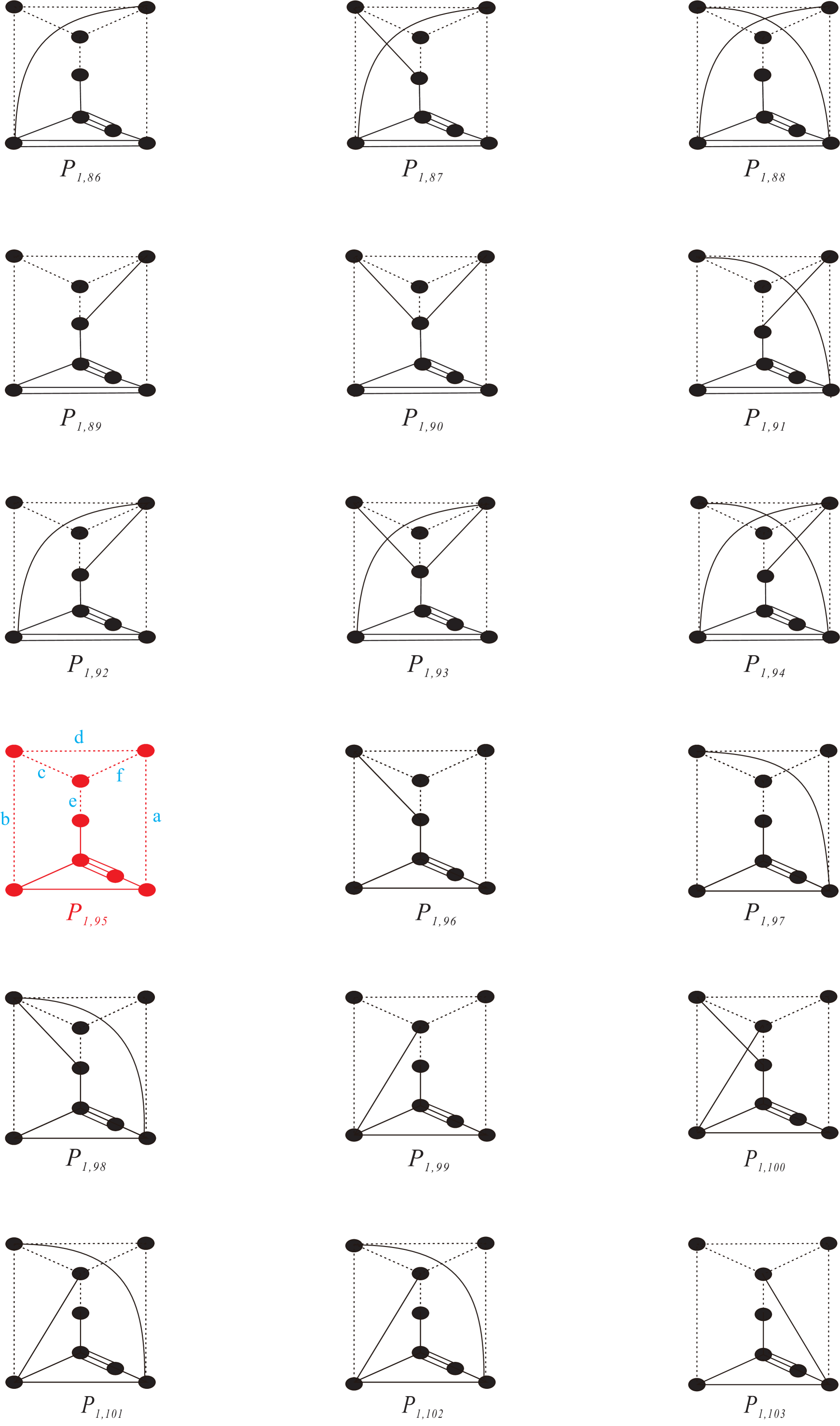
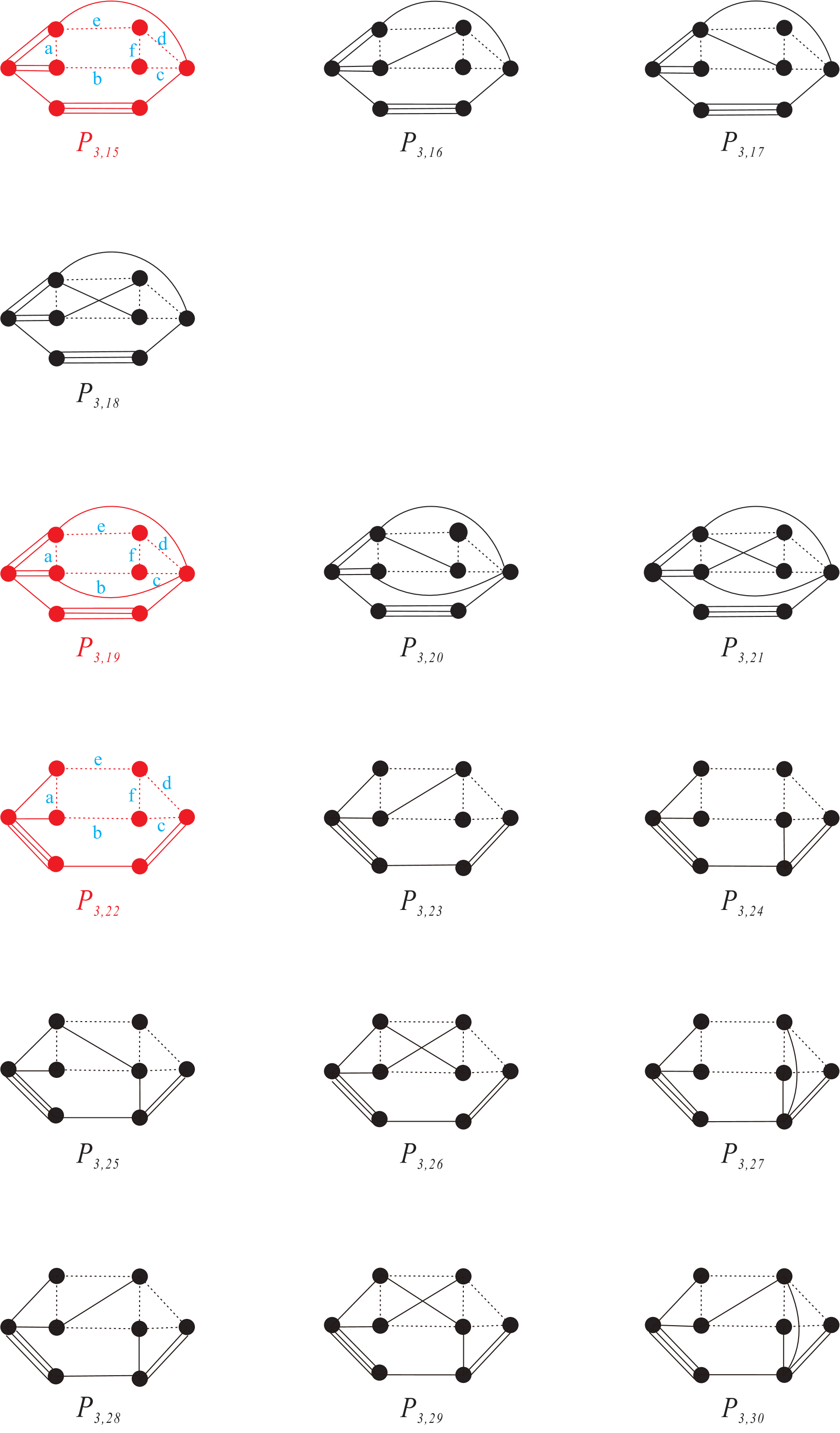
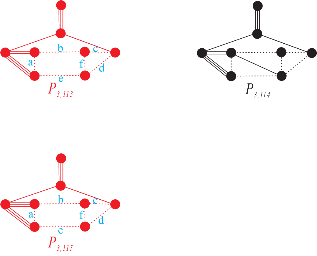
After conducting all of these procedures in Mathematica, we find that only fourteen of all simple $4$ -polytopes with $8$ facets admit compact hyperbolic structure. Besides, we can glue the $3$ -prism to seven of them. The results are reported in Table 6. The polytopes with labels in red are the “basis” polytopes, and the ones on last line can be obtained by gluing prism ends to those of the second line from the bottom. The Coxeter diagrams and length information are shown in the end of this paper (pages 22–55).


$d_{k}$	6			5					4			3
polytope	1	2	3	4	6	7	8	$13$	$16$	$17$	$34$	$18$	$21$	$26$
# (selected) SEILper potential	8	12	18	1	1	11	4	4	12	48	12	75	1	4
# gram (of basis vectors)	8	12	18	1	1	5	1	3	4	8	12	4	1	2
# gram after suitably gluing	130	49	115	2	1	15	2	N	N	N	N	N	N	N
$3$ -prisms to the orthoganal ends	130	49	115	2	1	15	2	N	N	N	N	N	N	N

Table 6. Results of the compact hyperbolic Coxeter

4

-polytopes with 8 facets. The value of polytope labeled by

13,16,17,34,18,21,

26

on the last line is “N”, which means the

l_{4}\_basis

set of

P_{13}

P_{16}

P_{17}

P_{34}

P_{18}

P_{21}

P_{26}

is empty and we are not be able to glue them with prism ends.

7. Validation and Results

1. “Basis Approach” vs. “Direct approach”.

We calculate SEILper potential matrices without using $l_{4}\_basis$ -conditions for those polytopes having $3$ -simplex facets. The numbers of Gram matrices corresponding to all of the possible compact hyperbolic polytopes and the results after the Mathematica round are reported in Table 7. They are the same as the previous work accomplished via “basis approach”.


grp	6			5

polytopes	1	2	3		4	6	7	8
#SEILper	130	49	115		571	26	8,579	5,258
#Gram	130	49	115		2	1	15	2

Table 7. Results obtained by direct approach.

2. The compact hyperbolic $4$ -cubes are in the family of compact hyperbolic Coxeter $4$ -polytope with 8 facets. We obtain the same results of exactly $12$ compact hyperbolic $4$ -cubes obtained by Jacquemet and Tschantz in [JT18] ³³3It seems that there is a small typo in Table $5$ of [JT18], where the lengths for $\Sigma_{2}^{2}$ and $\Sigma_{2}^{3}$ should be swapped. as shown in Figure 33.

3. Flikson and Turmarkin constructed 8 compact hyperbolic Coxeter polytopes with 8 facets in [FT14] as follows, which are exactly the eight bases of the polytope $P_{1}$ shown in red in Figure 10–17.

4. A. Burcroff obtained independently and confirmed the same result in [Bur22] after our mutual check. The correspondence of notions of the polytopes, which admit a hyperbolic structure, between our list and Burcroff’s are presented in Table 8.


MZ	1	2	3	4	6	7	8	13	16	17	18	21	26	34
A. Burcroff	$G_{1}$	$G_{3}$	$G_{2}$	$G_{7}$	$G_{8}$	$G_{9}$	$G_{6}$	$G_{5}$	$G_{13}$	$G_{11}$	$G_{12}$	$G_{10}$	$G_{14}$	$G_{4}$

Table 8. Notion correspondence between our list and the list in [Bur22].

1. Coxeter diagrams for $P_{1}$

	a	b	c
	d	e	f
$\displaystyle P_{1,1}$	$\displaystyle\frac{1}{2}\sqrt{5+3\sqrt{5}+4\sqrt{3+\sqrt{5}}}$	$\displaystyle\sqrt{\frac{1}{14}(11+6\sqrt{2}+\sqrt{5(9-4\sqrt{2})})}$	$\displaystyle\sqrt{\frac{1}{7}(10+4\sqrt{10}+\sqrt{253+80\sqrt{10}})}$
$\displaystyle P_{1,1}$	$\displaystyle\sqrt{\frac{1}{7}(5+4\sqrt{2})(2+\sqrt{5})}$	$\displaystyle\frac{1}{2}\sqrt{\frac{1}{2}(5+3\sqrt{5}+4\sqrt{3+\sqrt{5}})}$	$\displaystyle\frac{1}{2}\sqrt{9+4\sqrt{2}+\sqrt{5}}$
$\displaystyle P_{1,19}$	$\displaystyle\sqrt{\frac{61}{62}+\frac{5\sqrt{5}}{62}}$	$\displaystyle\sqrt{\frac{73}{38}+\frac{25\sqrt{5}}{38}}$	$\displaystyle 2\sqrt{\frac{1}{19}(8+3\sqrt{5})}$
$\displaystyle P_{1,19}$	$\displaystyle 3\sqrt{\frac{1}{589}(63+26\sqrt{5})}$	$\displaystyle\frac{1}{2}\sqrt{7+2\sqrt{5}}$	$\displaystyle\sqrt{\frac{74}{31}+\frac{33\sqrt{5}}{31}}$
$\displaystyle P_{1,28}$	$\displaystyle\sqrt{\frac{20}{11}+\frac{6\sqrt{5}}{11}}$	$\displaystyle\sqrt{\frac{20}{11}+\frac{6\sqrt{5}}{11}}$	$\displaystyle\sqrt{\frac{16}{11}+\frac{7\sqrt{5}}{11}}$
$\displaystyle P_{1,28}$	$\displaystyle\frac{3}{11}(3+2\sqrt{5})$	$\displaystyle\frac{1}{2}\sqrt{5+\sqrt{5}}$	$\displaystyle\sqrt{\frac{16}{11}+\frac{7\sqrt{5}}{11}}$
$\displaystyle P_{1,54}$	$\displaystyle\frac{1}{2}(1+\sqrt{5})$	$\displaystyle\frac{1}{2}(1+\sqrt{5})$	$\displaystyle\frac{1}{2}(1+\sqrt{5})$
$\displaystyle P_{1,54}$	$\displaystyle\frac{1}{2}(1+\sqrt{5})$	$\displaystyle\frac{1}{2}(1+\sqrt{5})$	$\displaystyle\frac{1}{2}(1+\sqrt{5})$
$\displaystyle P_{1,61}$	$\displaystyle\sqrt{\frac{23}{11}+\frac{8\sqrt{5}}{11}}$	$\displaystyle\sqrt{\frac{23}{11}+\frac{8\sqrt{5}}{11}}$	$\displaystyle\sqrt{\frac{23}{11}+\frac{8\sqrt{5}}{11}}$
$\displaystyle P_{1,61}$	$\displaystyle\frac{1}{11}(28+15\sqrt{5})$	$\displaystyle\frac{1}{2}(1+\sqrt{5})$	$\displaystyle\sqrt{\frac{23}{11}+\frac{8\sqrt{5}}{11}}$
$\displaystyle P_{1,71}$	$\displaystyle\sqrt{\frac{17}{22}+\frac{13}{22\sqrt{5}}}$	$\displaystyle\sqrt{\frac{42}{11}+\frac{17\sqrt{5}}{11}}$	$\displaystyle\sqrt{\frac{65}{22}+\frac{25\sqrt{5}}{22}}$
$\displaystyle P_{1,71}$	$\displaystyle\sqrt{\frac{13}{11}+\frac{2}{\sqrt{5}}}$	$\displaystyle\sqrt{\frac{19}{8}+\frac{7\sqrt{5}}{8}}$	$\displaystyle\sqrt{\frac{2}{55}(25+9\sqrt{5})}$
$\displaystyle P_{1,83}$	$\displaystyle\sqrt{\frac{1}{3}(1+\sqrt{10}-\sqrt{7-2\sqrt{10}})}$	$\displaystyle\sqrt{\frac{1}{2}(2+\sqrt{5}+\sqrt{7+3\sqrt{5}})}$	$\displaystyle\sqrt{\frac{1}{11}(24+6\sqrt{2}+5\sqrt{5}+4\sqrt{10})}$
$\displaystyle P_{1,83}$	$\displaystyle(\frac{13}{9}+\frac{4\sqrt{10}}{9})^{1/4}$	$\displaystyle\frac{2}{\sqrt{7+6\sqrt{2}-\sqrt{5}-4\sqrt{10}}}$	$\displaystyle\sqrt{\frac{1}{33}(1+28\sqrt{2}+4\sqrt{5}(2+\sqrt{2}))}$
$\displaystyle P_{1,95}$	$\displaystyle\frac{1}{4}(5+\sqrt{5})$	$\displaystyle\sqrt{\frac{65}{22}+\frac{25\sqrt{5}}{22}}$	$\displaystyle\sqrt{\frac{431}{341}+\frac{170\sqrt{5}}{341}}$
$\displaystyle P_{1,95}$	$\displaystyle\sqrt{\frac{26}{11}+\frac{10\sqrt{5}}{11}}$	$\displaystyle\sqrt{\frac{5}{31}(6+\sqrt{5})}$	$\displaystyle\sqrt{\frac{57}{62}+\frac{25\sqrt{5}}{62}}$

1. Coxeter diagrams for $P_{2}$

	a	b	c
	d	e	f
$\displaystyle P_{2,1}$	$\displaystyle\sqrt{\frac{2}{11}(7+\sqrt{5})}$	$\displaystyle\frac{1}{38}(16+6\sqrt{5}+19\sqrt{\frac{1728}{361}+\frac{496\sqrt{5}}{361}})$	$\displaystyle\frac{1}{19}(16+6\sqrt{5}+\sqrt{\frac{1}{2}(169-15\sqrt{5})})$
$\displaystyle P_{2,1}$	$\displaystyle\frac{1}{2}\sqrt{\frac{1}{2}(9+\sqrt{5})}$	$\displaystyle\frac{1}{19}\sqrt{\frac{1}{22}(22539+9889\sqrt{5}+4\sqrt{56071390+25075410\sqrt{5}})}$	$\displaystyle\frac{1}{19}\sqrt{\frac{1}{22}(76723+34293\sqrt{5}+4\sqrt{526827338+235604346\sqrt{5}})}$
$\displaystyle P_{2,13}$	$\displaystyle\frac{1}{2}\sqrt{\frac{1}{2}(9+\sqrt{5})}$	$\displaystyle\frac{1}{2}(3+\sqrt{5})$	$\displaystyle\sqrt{\frac{39}{8}+\frac{17\sqrt{5}}{8}}$
$\displaystyle P_{2,13}$	$\displaystyle\frac{1}{2}\sqrt{\frac{1}{2}(9+\sqrt{5})}$	$\displaystyle\sqrt{\frac{39}{8}+\frac{17\sqrt{5}}{8}}$	$\displaystyle\frac{1}{4}(11+5\sqrt{5})$
$\displaystyle P_{2,19}$	$\displaystyle\sqrt{\frac{2}{11}(7+\sqrt{5})}$	$\displaystyle\frac{1}{4}(5+\sqrt{5})$	$\displaystyle\sqrt{\frac{26}{11}+\frac{10\sqrt{5}}{11}}$
$\displaystyle P_{2,19}$	$\displaystyle\sqrt{\frac{2}{11}(7+\sqrt{5})}$	$\displaystyle\sqrt{\frac{26}{11}+\frac{10\sqrt{5}}{11}}$	$\displaystyle\frac{1}{11}(35+16\sqrt{5})$
$\displaystyle P_{2,29}$	$\displaystyle\frac{1}{2}(1+\sqrt{5})$	$\displaystyle 1+\frac{\sqrt{5}}{2}$	$\displaystyle\frac{1}{2}\sqrt{5(3+\sqrt{5})}$
$\displaystyle P_{2,29}$	$\displaystyle\frac{1}{2}(1+\sqrt{5})$	$\displaystyle\frac{1}{2}\sqrt{5(3+\sqrt{5})}$	$\displaystyle\frac{1}{2}(7+3\sqrt{5})$
$\displaystyle P_{2,32}$	$\displaystyle\sqrt{\frac{43}{38}+\frac{9\sqrt{5}}{38}}$	$\displaystyle\frac{1}{8}(13+3\sqrt{5})$	$\displaystyle\frac{1}{2}\sqrt{\frac{5}{38}(87+35\sqrt{5})}$
$\displaystyle P_{2,32}$	$\displaystyle\sqrt{\frac{43}{38}+\frac{9\sqrt{5}}{38}}$	$\displaystyle\frac{1}{2}\sqrt{\frac{5}{38}(87+35\sqrt{5})}$	$\displaystyle\frac{1}{38}(83+43\sqrt{5})$
$\displaystyle P_{2,33}$	$\displaystyle\frac{1}{2}\sqrt{5+\sqrt{5}}$	$\displaystyle\frac{1}{2}(3+\sqrt{5})$	$\displaystyle\sqrt{5+2\sqrt{5}}$
$\displaystyle P_{2,33}$	$\displaystyle\frac{1}{2}\sqrt{5+\sqrt{5}}$	$\displaystyle\sqrt{5+2\sqrt{5}}$	$\displaystyle\frac{1}{2}(7+3\sqrt{5})$
$\displaystyle P_{2,36}$	$\displaystyle\sqrt{\frac{1}{2}(2+\sqrt{5}+\sqrt{7+3\sqrt{5}})}$	$\displaystyle\frac{1}{4}(7+3\sqrt{5}+4\sqrt{3+\sqrt{5}})$	$\displaystyle\frac{1}{2}\sqrt{61+43\sqrt{2}+\sqrt{5(1451+1026\sqrt{2})}}$
$\displaystyle P_{2,36}$	$\displaystyle\sqrt{\frac{1}{2}(2+\sqrt{5}+\sqrt{7+3\sqrt{5}})}$	$\displaystyle\frac{1}{2}\sqrt{61+43\sqrt{2}+27\sqrt{5}+19\sqrt{10}}$	$\displaystyle\sqrt{2}(2+\sqrt{5})+\frac{3}{2}(3+\sqrt{5})$
$\displaystyle P_{2,39}$	$\displaystyle\sqrt{\frac{2}{19}(9+\sqrt{5})}$	$\displaystyle\frac{1}{22}\sqrt{1063+419\sqrt{5}+8\sqrt{29530+13204\sqrt{5}}}$	$\displaystyle\frac{1}{22}(26+10\sqrt{5}+11\sqrt{\frac{340}{121}+\frac{124\sqrt{5}}{121}})$
$\displaystyle P_{2,39}$	$\displaystyle\frac{1}{2}\sqrt{5+\sqrt{5}}$	$\displaystyle\frac{1}{11}\sqrt{\frac{1}{19}(5426+1707\sqrt{5}+8\sqrt{356050+159164\sqrt{5}})}$	$\displaystyle\frac{11}{\sqrt{4628-2011\sqrt{5}-4\sqrt{52445-22999\sqrt{5}}}}$
$\displaystyle P_{2,41}$	$\displaystyle\sqrt{\frac{43}{38}+\frac{9\sqrt{5}}{38}}$	$\displaystyle\frac{1}{4}\sqrt{23+9\sqrt{5}+2\sqrt{202+90\sqrt{5}}}$	$\displaystyle\frac{1}{4}(1+\sqrt{5}+2\sqrt{8+3\sqrt{5}})$
$\displaystyle P_{2,41}$	$\displaystyle\frac{1}{2}(1+\sqrt{5})$	$\displaystyle\frac{1}{2}\sqrt{\frac{1}{19}(143+37\sqrt{5}+2\sqrt{2442+1082\sqrt{5}})}$	$\displaystyle\sqrt{\frac{1}{38}(319+141\sqrt{5}+2\sqrt{43618+19506\sqrt{5}})}$
$\displaystyle P_{2,43}$	$\displaystyle\sqrt{\frac{2}{19}(9+\sqrt{5})}$	$\displaystyle 2+\frac{\sqrt{5}}{2}$	$\displaystyle\sqrt{\frac{78}{19}+\frac{34\sqrt{5}}{19}}$
$\displaystyle P_{2,43}$	$\displaystyle\sqrt{\frac{2}{19}(9+\sqrt{5})}$	$\displaystyle\sqrt{\frac{78}{19}+\frac{34\sqrt{5}}{19}}$	$\displaystyle\frac{1}{19}(47+20\sqrt{5})$
$\displaystyle P_{2,44}$	$\displaystyle 1.9923$	$\displaystyle 4.04306$	$\displaystyle 4.7181$
$\displaystyle P_{2,44}$	$\displaystyle 1.08754$	$\displaystyle 4.60491$	$\displaystyle 8.13984$
$\displaystyle P_{2,46}$	$\displaystyle 1.9923$	$\displaystyle 3.71598$	$\displaystyle 5.56213$
$\displaystyle P_{2,46}$	$\displaystyle 1.345$	$\displaystyle 4.25068$	$\displaystyle 9.72857$

Remark 7.1.

For $P_{2,44}$ , the acute solutions are:

$f=\displaystyle\frac{1}{11\sqrt{19}}\sqrt{22104+12082\sqrt{2}+9885\sqrt{5}+5400\sqrt{10}+4\sqrt{86889872+59414261\sqrt{2}+38858338\sqrt{5}+26570859\sqrt{10}}}$

$e=\sqrt{1-31f^{2}+14\sqrt{5}f^{2}}$

$b=\displaystyle\frac{1}{248}(-42-49\sqrt{2}-38\sqrt{5}-3\sqrt{10}+(5666+679\sqrt{2}-2538\sqrt{5}-295\sqrt{10})f^{2})$

$a=\displaystyle\frac{1}{1264}e(584+137\sqrt{2}+350\sqrt{5}+163\sqrt{10}+(50886+13227\sqrt{2}-22792\sqrt{5}-5903\sqrt{10})f^{2})$

$d=\displaystyle\frac{1}{1896}ef(30344+21847\sqrt{2}-12830\sqrt{5}-10679\sqrt{10}+19(-203414-160301\sqrt{2}+90964\sqrt{5}+71693\sqrt{10})f^{2})$

$c=\displaystyle\frac{1}{117552}ef(-1719980-1190961\sqrt{2}+844320\sqrt{5}+495395\sqrt{10}+(242831436+150419207\sqrt{2}-108605296\sqrt{5}$

$-67264185\sqrt{10})f^{2})$

For $P_{2,46}$ , the acute solutions are:

$f=\displaystyle\frac{1}{11\sqrt{2}}\sqrt{3358+1857\sqrt{2}+1498\sqrt{5}+831\sqrt{10}+2\sqrt{2(3804500+2601475\sqrt{2}+1701426\sqrt{5}+1163413\sqrt{10}}}$

$e=\displaystyle\sqrt{1-11f^{2}+5\sqrt{5}f^{2}}$

$d=\displaystyle\frac{1}{712}ef(-1188-100\sqrt{5}+547\sqrt{2}+85\sqrt{10}-3f^{2}(-51628+23074\sqrt{5}-39527\sqrt{2}+17687\sqrt{10}))$

$c=\displaystyle\frac{1}{22072}ef((-5147665-3402751\sqrt{2}+2303503\sqrt{5}+1520761\sqrt{10})f^{2}+(10517-15966\sqrt{2}+2905\sqrt{5}+935\sqrt{10}))$

$b=\displaystyle\frac{1}{124}(-22-36\sqrt{2}-14\sqrt{5}-6\sqrt{10}-69f^{2}-313\sqrt{2}f^{2}+35\sqrt{5}f^{2}+139\sqrt{10}f^{2})$

$a=\displaystyle\frac{1}{356}e(171+313\sqrt{2}+9\sqrt{5}-21\sqrt{10}+(-10376-9016\sqrt{2}+4644\sqrt{5}+4027\sqrt{10})f^{2})$

3. Coxeter diagrams for $P_{3}$

	$a$	$b$	$c$
	$d$	$e$	$f$
$P_{3,1}$	$\frac{3}{11}(3+2\sqrt{5})$	$\frac{2}{11}\sqrt{265+118\sqrt{5}}$	$\frac{1}{2}\sqrt{5+\sqrt{5}}$
$P_{3,1}$	$\frac{1}{2}\sqrt{5+\sqrt{5}}$	$\frac{2}{11}\sqrt{265+118\sqrt{5}}$	$\frac{7}{11}(3+2\sqrt{5})$
$P_{3,4}$	$\frac{1}{11}(17+4\sqrt{5})$	$\sqrt{\frac{17208}{2299}+\frac{7688\sqrt{5}}{2299}}$	$\sqrt{\frac{2}{19}(9+\sqrt{5})}$
$P_{3,4}$	$\sqrt{\frac{2}{19}(9+\sqrt{5})}$	$\sqrt{\frac{17208}{2299}+\frac{7688\sqrt{5}}{2299}}$	$\frac{1}{209}(257+208\sqrt{5})$
$P_{3,5}$	$\frac{1}{19}(17+4\sqrt{5})$	$\sqrt{\frac{20936}{3971}+\frac{9352\sqrt{5}}{3971}}$	$\sqrt{\frac{2}{11}(7+\sqrt{5})}$
$P_{3,5}$	$\sqrt{\frac{2}{11}(7+\sqrt{5})}$	$\sqrt{\frac{20936}{3971}+\frac{9352\sqrt{5}}{3971}}$	$\frac{1}{209}(257+208\sqrt{5})$
$P_{3,15}$	$3.54605$	$5.88536$	$1.9923$
$P_{3,15}$	$1.345$	$5.88536$	$6.61923$
$P_{3,19}$	$\frac{1}{11}(8+13\sqrt{2}+9\sqrt{5}+5\sqrt{10})$	$\frac{1}{11}\sqrt{2074+1462\sqrt{2}+950\sqrt{5}+630\sqrt{10}}$	$\sqrt{\frac{1}{2}(2+\sqrt{5}+\sqrt{7+3\sqrt{5}})}$
$P_{3,19}$	$\sqrt{\frac{1}{2}(2+\sqrt{5}+\sqrt{7+3\sqrt{5}})}$	$\frac{1}{11}\sqrt{2074+1462\sqrt{2}+950\sqrt{5}+630\sqrt{10}}$	$\frac{1}{11}(37+12\sqrt{2}+2\sqrt{5}(5+4\sqrt{2}))$
$P_{3,22}$	$\frac{1}{2}(3+\sqrt{5})$	$\sqrt{\frac{115}{11}+\frac{51\sqrt{5}}{11}}$	$\sqrt{\frac{10}{11}+\frac{3\sqrt{5}}{11}}$
$P_{3,22}$	$\sqrt{\frac{10}{11}+\frac{3\sqrt{5}}{11}}$	$\sqrt{\frac{115}{11}+\frac{51\sqrt{5}}{11}}$	$\frac{7}{11}(3+2\sqrt{5})$
$P_{3,32}$	$4.41427$	$6.42282$	$1.82559$
$P_{3,32}$	$1.23245$	$6.42282$	$6.61923$
$P_{3,48}$	$1+\sqrt{5}+\sqrt{7+3\sqrt{5}}$	$\sqrt{\frac{1}{11}(222+161\sqrt{2}+104\sqrt{5}+67\sqrt{10})}$	$\sqrt{\frac{1}{22}(19+9\sqrt{5}+2\sqrt{147+65\sqrt{5}})}$
$P_{3,48}$	$\sqrt{\frac{1}{22}(19+9\sqrt{5}+2\sqrt{147+65\sqrt{5}})}$	$\sqrt{\frac{1}{11}(222+161\sqrt{2}+104\sqrt{5}+67\sqrt{10})}$	$\frac{1}{11}(37+12\sqrt{2}+2\sqrt{5}(5+4\sqrt{2}))$
$P_{3,58}$	$\frac{1}{76}(25+7\sqrt{5}+8\sqrt{108+31\sqrt{5}})$	$\frac{1}{19}\sqrt{\frac{1}{22}(30747+13689\sqrt{5}+8\sqrt{29359122+13129762\sqrt{5}})}$	$\sqrt{\frac{2}{11}(7+\sqrt{5})}$
$P_{3,58}$	$\frac{1}{2}\sqrt{\frac{1}{2}(9+\sqrt{5})}$	$\frac{1}{38}(32+12\sqrt{5}+19\sqrt{\frac{1592}{361}+\frac{711\sqrt{5}}{361}})$	$\frac{1}{19}\sqrt{\frac{1}{22}(26791+8529\sqrt{5}+8\sqrt{11214278+5015082\sqrt{5}})}$
$P_{3,70}$	$5.67675$	$7.83841$	$1.82559$
$P_{3,70}$	$1.14412$	$6.04875$	$6.24279$
$P_{3,82}$	$\frac{1}{11}\sqrt{197+69\sqrt{5}+4\sqrt{2(845+358\sqrt{5})}}$	$\frac{1}{11}\sqrt{\frac{1}{19}(7186+3203\sqrt{5}+4\sqrt{6387730+2856676\sqrt{5}}}$	$\sqrt{\frac{2}{19}(9+\sqrt{5})}$
$P_{3,82}$	$\frac{1}{2}\sqrt{5+\sqrt{5}}$	$\frac{1}{22}(26+10\sqrt{5}+11\sqrt{\frac{1385}{121}+\frac{619\sqrt{5}}{121})}$	$\frac{1}{11}\sqrt{\frac{1}{19}(11128+3983\sqrt{5}+8\sqrt{2439905+1091149\sqrt{5}})}$
$P_{3,84}$	$3.84864$	$4.97946$	$1.08754$
$P_{3,84}$	$1.9923$	$6.47518$	$5.62568$
$P_{3,86}$	$\frac{3}{4}+\frac{\sqrt{5}}{4}+\sqrt{\frac{5}{2}+\sqrt{5}}$	$1+\frac{\sqrt{5}}{2}+\sqrt{\frac{5}{2}+\sqrt{5}}$	$\frac{1}{2}\sqrt{3+\sqrt{5}}$
$P_{3,86}$	$\frac{1}{\sqrt{2-\frac{3}{\sqrt{5}}}}$	$\sqrt{\frac{1}{22}(173+75\sqrt{5}+4\sqrt{3625+1621\sqrt{5}})}$	$\sqrt{\frac{1}{22}(123+49\sqrt{5}+4\sqrt{1385+619\sqrt{5}})}$
$P_{3,98}$	$\frac{3}{19}(8+3\sqrt{5})$	$\frac{1}{19}\sqrt{2442+1082\sqrt{5}}$	$\frac{1}{2}\sqrt{\frac{1}{2}(9+\sqrt{5})}$
$P_{3,98}$	$\frac{1}{2}\sqrt{\frac{1}{2}(9+\sqrt{5})}$	$\frac{1}{19}\sqrt{2442+1082\sqrt{5}}$	$\frac{1}{19}(20+17\sqrt{5})$
$P_{3,104}$	$2+\sqrt{5}$	$3+\sqrt{5}$	$\frac{1}{2}\sqrt{3+\sqrt{5}}$
$P_{3,104}$	$\frac{1}{2}\sqrt{3+\sqrt{5}}$	$3+\sqrt{5}$	$2+\sqrt{5}$
$P_{3,110}$	$\frac{1}{2}(1+\sqrt{5})$	$\sqrt{7+3\sqrt{5}}$	$\frac{1}{2}(1+\sqrt{5})$
$P_{3,110}$	$\frac{1}{2}(1+\sqrt{5})$	$\sqrt{7+3\sqrt{5}}$	$2+\sqrt{5}$
$P_{3,113}$	$\frac{1}{2}\sqrt{\frac{3}{2}(3+\sqrt{5})+\sqrt{8+3\sqrt{5}}}$	$\sqrt{\frac{1}{38}(94+40\sqrt{5}+\sqrt{2(8331+3725\sqrt{5})})}$	$\sqrt{\frac{43}{38}+\frac{9\sqrt{5}}{38}}$
$P_{3,113}$	$\frac{1}{2}(1+\sqrt{5})$	$\frac{1}{2}(2+\sqrt{5}+\sqrt{8+3\sqrt{5})}$	$\sqrt{\frac{1}{19}(8+3\sqrt{5})(9+2\sqrt{8+3\sqrt{5})}}$
$P_{3,115}$	$\frac{1}{4}(5+\sqrt{5})$	$\sqrt{\frac{109}{19}+\frac{48\sqrt{5}}{19}}$	$\sqrt{\frac{43}{38}+\frac{9\sqrt{5}}{38}}$
$P_{3,115}$	$\sqrt{\frac{43}{38}+\frac{9\sqrt{5}}{38}}$	$\sqrt{\frac{109}{19}+\frac{48\sqrt{5}}{19}}$	$\frac{1}{19}(20+17\sqrt{5})$

Remark 7.2.

For $P_{3,15}$ , the acute solutions are:

$f=\frac{1}{11}\sqrt{799+406\sqrt{2}+364\sqrt{5}+168\sqrt{10}+2\sqrt{2(211980+145015\sqrt{2}+94834\sqrt{5}+64817\sqrt{10}}}$

$e=\frac{1}{2}\sqrt{-1-\sqrt{5}+f^{2}+\sqrt{5}f^{2}}$

$d={\displaystyle\frac{1}{496}}e(1248+161\sqrt{2}+240\sqrt{5}+67\sqrt{10}+(140+81\sqrt{2}-3\sqrt{5}(36+7\sqrt{2}))f^{2})$

$c={\displaystyle\frac{1}{1488}}ef(4396+1661\sqrt{2}+436\sqrt{5}+511\sqrt{10}+(-896-1327\sqrt{2}+304\sqrt{5}+595\sqrt{10})f^{2})$

$b={\displaystyle\frac{1}{186}}ef(248+211\sqrt{2}-31\sqrt{5}-94\sqrt{10}+(-1000-443\sqrt{2}+443\sqrt{5}+200\sqrt{10})f^{2})$

$a={\displaystyle\frac{1}{248}}(-259+13\sqrt{2}-7\sqrt{5}-3\sqrt{10}+(37+69\sqrt{2}+\sqrt{5}-35\sqrt{10})f^{2})$

For $P_{3,32}$ , the acute solutions are:

$f=\frac{1}{11}\sqrt{799+406\sqrt{2}+364\sqrt{5}+168\sqrt{10}+2\sqrt{2(211980+145015\sqrt{2}+94834\sqrt{5}+64817\sqrt{10}}}$

$e={\displaystyle\frac{1}{2\sqrt{2}}}\sqrt{-1-3\sqrt{5}+f^{2}+3\sqrt{5}f^{2}}$

$d={\displaystyle\frac{1}{2728}}e(4968+731\sqrt{2}+1464\sqrt{5}+315\sqrt{10}+11(20-28\sqrt{5}-3\sqrt{2}(-7+\sqrt{5}))f^{2})$

$c={\displaystyle\frac{1}{8184}}ef(16476+7091\sqrt{2}+3724\sqrt{5}+2619\sqrt{10}+11(-216-287\sqrt{2}+56\sqrt{5}+129\sqrt{10})f^{2})$

$b={\displaystyle\frac{1}{186}}ef(248+211\sqrt{2}-31\sqrt{5}-94\sqrt{10}+(-1000-443\sqrt{2}+443\sqrt{5}+200\sqrt{10})f^{2})$

$a={\displaystyle\frac{1}{496}}(-517+53\sqrt{2}-19\sqrt{5}-17\sqrt{10}+(127+329\sqrt{2}-15\sqrt{5}-157\sqrt{10})f^{2})$

For $P_{3,70}$ , the acute solutions are:

$f={\displaystyle\frac{1}{\sqrt{22}}}\sqrt{135+64\sqrt{2}+57\sqrt{5}+28\sqrt{10}+4\sqrt{2743+1884\sqrt{2}+1231\sqrt{5}+838\sqrt{10}}}$

$e={\displaystyle\frac{1}{2\sqrt{2}}}\sqrt{-1-3\sqrt{5}+f^{2}+3\sqrt{5}f^{2}}$

$d={\displaystyle\frac{1}{23684}}e(36906+2881\sqrt{2}+11886\sqrt{5}+847\sqrt{10}+(4504+3808\sqrt{2}-4044\sqrt{5}-874\sqrt{10})f^{2}$

$c={\displaystyle\frac{1}{2913132}}((2545015+877512\sqrt{2}+2315748\sqrt{5}+1194982\sqrt{10})ef+(2442218+1364747\sqrt{2}-1270198\sqrt{5}-$

$586721\sqrt{10})ef^{3})$

$b={\displaystyle\frac{1}{3813}}((6454+4099\sqrt{2}-743\sqrt{5}-1864\sqrt{10})ef+\frac{1}{2}(-8619-7529\sqrt{2}+3601\sqrt{5}+3483\sqrt{10})ef^{3})$

$a={\displaystyle\frac{1}{248}}(-97-15\sqrt{2}-73\sqrt{5}+13\sqrt{10}+(21-53\sqrt{2}+19\sqrt{5}+17\sqrt{10})f^{2})$

For $P_{3,84}$ , the acute solutions are:

$f={\displaystyle\frac{1}{11\sqrt{19}}}\sqrt{11104+5702\sqrt{2}+5133\sqrt{5}+2276\sqrt{10}+8\sqrt{4842088+3311169\sqrt{2}+2165554\sqrt{5}+1480687\sqrt{10}}}$

$e={\displaystyle\frac{1}{2}}\sqrt{-1-2\sqrt{5}+f^{2}+2\sqrt{5}f^{2}}$

$d={\displaystyle\frac{1}{24216}}e(-17104+5893\sqrt{2}-3602\sqrt{5}-20597\sqrt{10}+(-115066-24517\sqrt{2}+50384\sqrt{5}+12469\sqrt{10})f^{2})$

c= ${\displaystyle\frac{1}{1937062056}}ef(9466659574+914636627\sqrt{2}-3948733168\sqrt{5}-1618127971\sqrt{10}+(-23059580156-23947802279\sqrt{2}+$

$10158748906\sqrt{5}+10850958719\sqrt{10})f^{2})$

$b={\displaystyle\frac{1}{9918884}}ef(-31360330-1617047\sqrt{2}+13795674\sqrt{5}+3094731\sqrt{10}+(61953682+76754869\sqrt{2}-5\sqrt{5}(5508882+$

$6899345\sqrt{2}))f^{2})$

$a={\displaystyle\frac{1}{248}}(-57+\frac{177}{\sqrt{2}}-265\sqrt{\frac{5}{2}}+37\sqrt{5}+(-679-\frac{117}{\sqrt{2}}+89\sqrt{\frac{5}{2}}+295\sqrt{5})f^{2})$

	a	b	c	d	e
$\displaystyle P_{4,1}$	$\displaystyle\frac{1}{2}\sqrt{3(3+\sqrt{5})}$	$\displaystyle\sqrt{\frac{3}{19}(8+3\sqrt{5})}$	$\displaystyle\frac{1}{2}\sqrt{7+3\sqrt{5}}$	$\displaystyle\sqrt{\frac{2}{19}(8+3\sqrt{5})}$	$\displaystyle\sqrt{\frac{5}{19}(8+3\sqrt{5})}$
$\displaystyle P_{4,2}$	$\displaystyle\frac{1}{4}\sqrt{57+23\sqrt{5}+4\sqrt{30(9+4\sqrt{5})}}$	$\displaystyle\sqrt{\frac{24}{19}+\frac{9\sqrt{5}}{19}}$	$\displaystyle\frac{1}{4}(2(2+\sqrt{5})+\sqrt{21+9\sqrt{5}})$	$\displaystyle\sqrt{\frac{16}{19}+\frac{6\sqrt{5}}{19}}$	$\displaystyle\frac{1}{2}\sqrt{\frac{1}{19}(249+91\sqrt{5}+60\sqrt{6}+32\sqrt{30})}$
$\displaystyle P_{6,1}$	$\displaystyle\sqrt{\frac{5}{19}(8+3\sqrt{5})}$	$\displaystyle\sqrt{\frac{5}{19}(8+3\sqrt{5})}$	$\displaystyle\sqrt{\frac{5}{38}(9+\sqrt{5})}$	$\displaystyle\sqrt{\frac{5}{38}(9+\sqrt{5})}$	$\displaystyle\frac{25}{19}(9+\sqrt{5})-9$
$\displaystyle P_{8,1}$	$\displaystyle\frac{1}{2}\sqrt{5+\sqrt{5}}$	$\displaystyle\frac{1}{2}(3+\sqrt{5})$	$\displaystyle\frac{1}{2}(1+\sqrt{5})$	$\displaystyle\sqrt{5+2\sqrt{5}}$
$\displaystyle P_{8,2}$	$\displaystyle\frac{1}{2}(1+\sqrt{5+2\sqrt{5}})$	$\displaystyle\sqrt{7+3\sqrt{5}+\sqrt{85+38\sqrt{5}}}$	$\displaystyle\frac{1}{2}(1+\sqrt{5})$	$\displaystyle\frac{1}{2}\sqrt{43+19\sqrt{5}+2\sqrt{890+398\sqrt{5}}}$
$\displaystyle P_{13,1}$	$\displaystyle\frac{1}{2}\sqrt{3+\sqrt{2}}$	$\displaystyle\frac{1}{2}\sqrt{3+\sqrt{2}}$	$\displaystyle\frac{1}{2}(2+\sqrt{2})$	$\displaystyle 1+\sqrt{2}$	$\displaystyle\frac{1}{2}(2+\sqrt{2})$
$\displaystyle P_{13,2}$	$\displaystyle\sqrt{\frac{17}{23}+\frac{8\sqrt{2}}{23}}$	$\displaystyle\frac{1}{2}+\frac{1}{\sqrt{2}}$	$\displaystyle\frac{3}{2}+\frac{1}{\sqrt{2}}$	$\displaystyle 1+\frac{1}{\sqrt{2}}$	$\displaystyle\sqrt{\frac{17}{23}+\frac{8\sqrt{2}}{23}}$
$\displaystyle P_{13,3}$	$\displaystyle\sqrt{\frac{17}{23}+\frac{8\sqrt{2}}{23}}$	$\displaystyle\sqrt{\frac{17}{23}+\frac{8\sqrt{2}}{23}}$	$\displaystyle 1+\frac{1}{2\sqrt{2}}$	$\displaystyle 1+\frac{3}{2\sqrt{2}}$	$\displaystyle 1+\frac{1}{\sqrt{2}}$
$\displaystyle P_{16,1}$	$\displaystyle\sqrt{1+\frac{1}{\sqrt{2}}}$	$\displaystyle\sqrt{1+\frac{1}{\sqrt{2}}}$	$\displaystyle\sqrt{1+\frac{1}{\sqrt{2}}}$	$\displaystyle\sqrt{1+\frac{1}{\sqrt{2}}}$
$\displaystyle P_{16,2}$	$\displaystyle 2+\sqrt{2}$	$\displaystyle\sqrt{\frac{13}{7}+\frac{9\sqrt{2}}{7}}$	$\displaystyle\sqrt{\frac{2}{7}(3+\sqrt{2})}$	$\displaystyle 1+\frac{1}{\sqrt{2}}$
$\displaystyle P_{16,3}$	$\displaystyle\sqrt{1+\frac{1}{\sqrt{2}}}$	$\displaystyle\sqrt{1+\frac{1}{\sqrt{2}}}$	$\displaystyle\sqrt{1+\frac{1}{\sqrt{2}}}$	$\displaystyle\sqrt{1+\frac{1}{\sqrt{2}}}$
$\displaystyle P_{16,4}$	$\displaystyle\sqrt{\frac{13}{7}+\frac{9\sqrt{2}}{7}}$	$\displaystyle 2+\sqrt{2}$	$\displaystyle 1+\frac{1}{\sqrt{2}}$	$\displaystyle\sqrt{\frac{2}{7}(3+\sqrt{2})}$

	a	b	c
	d	e
$\displaystyle P_{7,1}$	$\displaystyle\sqrt{\frac{23}{8}+\frac{9\sqrt{5}}{8}}$	$\displaystyle\frac{1}{2}\sqrt{\frac{1}{2}(6+\sqrt{5})}$	$\displaystyle\frac{1}{4}\sqrt{5(3+\sqrt{5})}$
$\displaystyle P_{7,1}$	$\displaystyle\frac{1}{2}(1+\sqrt{5})$	$\displaystyle\sqrt{\frac{23}{8}+\frac{9\sqrt{5}}{8}}$
$\displaystyle P_{7,2}$	$\displaystyle\frac{1}{8}(3(1+\sqrt{5})+\sqrt{206+86\sqrt{5}})$	$\displaystyle\frac{1}{2}\sqrt{\frac{1}{2}(6+\sqrt{5})}$	$\displaystyle\frac{1}{4}\sqrt{22+\frac{17\sqrt{5}}{2}+\sqrt{655+290\sqrt{5}}}$
$\displaystyle P_{7,2}$	$\displaystyle\frac{1}{2}(1+\sqrt{5})$	$\displaystyle\frac{1}{8}(5+\sqrt{5}+\sqrt{206+86\sqrt{5}})$
$\displaystyle P_{7,3}$	$\displaystyle\frac{1}{8}(5+3\sqrt{5}+\sqrt{206+86\sqrt{5}})$	$\displaystyle\frac{1}{2}\sqrt{\frac{1}{2}(6+\sqrt{5})}$	$\displaystyle\frac{1}{4}\sqrt{\frac{1}{2}(39+11\sqrt{5}+\sqrt{470+130\sqrt{5}})}$
$\displaystyle P_{7,3}$	$\displaystyle\frac{1}{2}(1+\sqrt{5})$	$\displaystyle\frac{1}{8}(5+3\sqrt{5}+\sqrt{206+86\sqrt{5}})$
$\displaystyle P_{7,4}$	$\displaystyle 1+\sqrt{2}$	$\displaystyle 1+\frac{1}{2\sqrt{2}}$	$\displaystyle 1+\frac{1}{\sqrt{2}}$
$\displaystyle P_{7,4}$	$\displaystyle\sqrt{\frac{9}{14}+\frac{2\sqrt{2}}{7}}$	$\displaystyle\sqrt{\frac{1}{7}(9+4\sqrt{2})}$
$\displaystyle P_{7,5}$	$\displaystyle 1+\frac{1}{\sqrt{2}}+\sqrt{\frac{26}{7}+\frac{18\sqrt{2}}{7}}$	$\displaystyle 1+\frac{1}{2\sqrt{2}}$	$\displaystyle\frac{1}{14}(7+7\sqrt{2}+2\sqrt{91+63\sqrt{2}})$
$\displaystyle P_{7,5}$	$\displaystyle\sqrt{\frac{9}{14}+\frac{2\sqrt{2}}{7}}$	$\displaystyle\sqrt{\frac{2}{7}(6+3\sqrt{2}+2\sqrt{5+3\sqrt{2}})}$
$\displaystyle P_{7,6}$	$\displaystyle 1+\frac{1}{\sqrt{2}}+\sqrt{\frac{26}{7}+\frac{18\sqrt{2}}{7}}$	$\displaystyle 1+\frac{1}{2\sqrt{2}}$	$\displaystyle\frac{1}{2}(\sqrt{2}+\sqrt{\frac{52}{7}+\frac{36\sqrt{2}}{7}})$
$\displaystyle P_{7,6}$	$\displaystyle\sqrt{\frac{9}{14}+\frac{2\sqrt{2}}{7}}$	$\displaystyle\sqrt{\frac{1}{7}(13+8\sqrt{2}+2\sqrt{54+38\sqrt{2}})}$
$\displaystyle P_{7,7}$	$\displaystyle\sqrt{\frac{1}{31}(29+10\sqrt{5})}$	$\displaystyle\frac{1}{2}\sqrt{4+\sqrt{5}}$	$\displaystyle\sqrt{\frac{1}{31}(23+9\sqrt{5})}$
$\displaystyle P_{7,7}$	$\displaystyle\frac{1}{2}(1+\sqrt{5})$	$\displaystyle\sqrt{\frac{2}{31}(29+10\sqrt{5})}$
$\displaystyle P_{7,8}$	$\displaystyle\frac{1}{62}\sqrt{4347+1577\sqrt{5}+8\sqrt{11(21727+9289\sqrt{5})}}$	$\displaystyle\frac{1}{2}\sqrt{4+\sqrt{5}}$	$\displaystyle\frac{1}{62}\sqrt{\frac{1}{2}(7899+2851\sqrt{5}+48\sqrt{29048+12674\sqrt{5}})}$
$\displaystyle P_{7,8}$	$\displaystyle\frac{1}{2}(1+\sqrt{5})$	$\displaystyle\frac{1}{124}(49+3\sqrt{5}+8\sqrt{448+178\sqrt{5}}$
$\displaystyle P_{7,9}$	$\displaystyle\frac{1}{31}\sqrt{1079+433\sqrt{5}+4\sqrt{75257+33535\sqrt{5}}}$	$\displaystyle\frac{1}{2}\sqrt{4+\sqrt{5}}$	$\displaystyle\frac{1}{31}\sqrt{968+213\sqrt{5}+4\sqrt{6613+787\sqrt{5}}}$
$\displaystyle P_{7,9}$	$\displaystyle\frac{1}{2}(1+\sqrt{5})$	$\displaystyle\frac{1}{62}(22+14\sqrt{5}+31\sqrt{\frac{7168}{961}+\frac{2848\sqrt{5}}{961}})$
$\displaystyle P_{7,10}$	$\displaystyle\sqrt{\frac{13}{7}+\frac{9\sqrt{2}}{7}}$	$\displaystyle\frac{1}{2}+\frac{1}{\sqrt{2}}$	$\displaystyle 2\sqrt{\frac{1}{7}(3+\sqrt{2})}$
$\displaystyle P_{7,10}$	$\displaystyle 1+\frac{1}{\sqrt{2}}$	$\displaystyle\sqrt{\frac{45}{7}+\frac{29\sqrt{2}}{7}}$
$\displaystyle P_{7,11}$	$\displaystyle 2+\sqrt{2}$	$\displaystyle\frac{1}{2}+\frac{1}{\sqrt{2}}$	$\displaystyle 1+\sqrt{2}$
$\displaystyle P_{7,11}$	$\displaystyle 1+\frac{1}{\sqrt{2}}$	$\displaystyle 3+\frac{5}{\sqrt{2}}$
$\displaystyle P_{7,12}$	$\displaystyle\frac{1}{14}(25+13\sqrt{2})$	$\displaystyle\frac{1}{2}+\frac{1}{\sqrt{2}}$	$\displaystyle\frac{8}{7}+\frac{17}{7\sqrt{2}}$
$\displaystyle P_{7,12}$	$\displaystyle 1+\frac{1}{\sqrt{2}}$	$\displaystyle\frac{1}{14}(41+37\sqrt{2})$
$\displaystyle P_{7,13}$	$\displaystyle 1+\sqrt{2}$	$\displaystyle\frac{1}{2}+\frac{1}{\sqrt{2}}$	$\displaystyle 1+\sqrt{2}$
$\displaystyle P_{7,13}$	$\displaystyle\sqrt{\frac{9}{14}+\frac{2\sqrt{2}}{7}}$	$\displaystyle\sqrt{\frac{9}{7}+\frac{4\sqrt{2}}{7}}$
$\displaystyle P_{7,14}$	$\displaystyle 1+\frac{1}{\sqrt{2}}+\sqrt{\frac{26}{7}+\frac{18\sqrt{2}}{7}}$	$\displaystyle\frac{1}{2}+\frac{1}{\sqrt{2}}$	$\displaystyle\frac{1}{2}+\frac{1}{\sqrt{2}}+\sqrt{\frac{26}{7}+\frac{18\sqrt{2}}{7}}$
$\displaystyle P_{7,14}$	$\displaystyle\sqrt{\frac{9}{14}+\frac{2\sqrt{2}}{7}}$	$\displaystyle\sqrt{\frac{1}{7}(13+8\sqrt{2}+2\sqrt{54+38\sqrt{2}})}$
$\displaystyle P_{7,15}$	$\displaystyle 1+\frac{1}{\sqrt{2}}+\sqrt{\frac{26}{7}+\frac{18\sqrt{2}}{7}}$	$\displaystyle\frac{1}{2}+\frac{1}{\sqrt{2}}$	$\displaystyle 1+\frac{1}{\sqrt{2}}+\sqrt{\frac{26}{7}+\frac{18\sqrt{2}}{7}}$
$\displaystyle P_{7,15}$	$\displaystyle\sqrt{\frac{9}{14}+\frac{2\sqrt{2}}{7}}$	$\displaystyle\sqrt{\frac{2}{7}(6+3\sqrt{2}+2\sqrt{5+3\sqrt{2}})}$

	$a$	$b$	$c$	$d$
$P_{17,1}$	$\displaystyle\frac{1}{2}(1+\sqrt{5})$	$\displaystyle\frac{1}{4}(3+\sqrt{5})$	$\displaystyle\frac{1}{2}(1+\sqrt{5})$	$\displaystyle\frac{1}{2}(1+\sqrt{5})$
$P_{17,2}$	$\displaystyle 1+\frac{1}{\sqrt{2}}$	$\displaystyle\frac{1}{2}+\frac{1}{\sqrt{2}}$	$\displaystyle 1+\frac{1}{\sqrt{2}}$	$\displaystyle\frac{3}{2}+\frac{1}{\sqrt{2}}$
$P_{17,3}$	$\displaystyle 1+\frac{1}{\sqrt{2}}$	$\displaystyle\frac{1}{2}+\frac{1}{\sqrt{2}}$	$\displaystyle 1+\frac{1}{\sqrt{2}}$	$\displaystyle\frac{3}{2}+\frac{1}{\sqrt{2}}$
$P_{17,4}$	$\displaystyle\frac{1}{2}(1+\sqrt{5})$	$\displaystyle\frac{1}{2}\sqrt{3+\frac{3}{\sqrt{5}}}$	$\displaystyle\frac{1}{2}(1+\sqrt{5})$	$\displaystyle\frac{1}{2}(1+\sqrt{5})$
$P_{17,5}$	$\displaystyle\frac{1}{2}(1+\sqrt{5})$	$\displaystyle\frac{1}{10}(5+3\sqrt{5})$	$\displaystyle\frac{1}{2}(1+\sqrt{5})$	$\displaystyle\frac{1}{2}(1+\sqrt{5})$
$P_{17,6}$	$\displaystyle\frac{1}{2}(1+\sqrt{5})$	$\displaystyle\frac{1}{2}\sqrt{3+\sqrt{5}}$	$\displaystyle\frac{1}{2}(1+\sqrt{5})$	$\displaystyle\frac{1}{2}(3+\sqrt{5})$
$P_{17,7}$	$\displaystyle\frac{1}{2}(1+\sqrt{5})$	$\displaystyle\frac{1}{2}(1+\sqrt{5})$	$\displaystyle\frac{1}{2}(1+\sqrt{5})$	$\displaystyle\frac{1}{2}(3+\sqrt{5})$
$P_{17,8}$	$\displaystyle\frac{1}{\sqrt{2}}(2\cos\frac{\pi}{7}(1+2\cos\frac{\pi}{7})-1)$	$\displaystyle 2\cos^{2}\frac{\pi}{7}-\frac{1}{2}$	$\displaystyle\frac{1}{\sqrt{2}}(2\cos\frac{\pi}{7}(1+2\cos\frac{\pi}{7})-1)$	$\displaystyle 2\cos\frac{\pi}{7}(1+2\cos\frac{\pi}{7})$
$P_{18,1}$	$2+\sqrt{2}$	$2+\sqrt{2}$	$5+4\sqrt{2}$
$P_{18,2}$	$\sqrt{2+\sqrt{2}}$	$\sqrt{2+\sqrt{2}}$	$1+\sqrt{2}$
$P_{18,3}$	$2+\sqrt{2}$	$2+\sqrt{2}$	$5+4\sqrt{2}$
$P_{18,4}$	$\sqrt{2+\sqrt{2}}$	$\sqrt{2+\sqrt{2}}$	$1+\sqrt{2}$
$P_{26,1}$	$\sqrt{1+\frac{1}{\sqrt{2}}}$	$\sqrt{1+\frac{1}{\sqrt{2}}}$	$\sqrt{1+\frac{1}{\sqrt{2}}}$
$P_{26,2}$	$\sqrt{1+\frac{1}{\sqrt{2}}}$	$\sqrt{1+\frac{1}{\sqrt{2}}}$	$\sqrt{1+\frac{1}{\sqrt{2}}}$

	$a$	$b$	$c$	$d$
$P_{34,1}$	$\frac{1}{4}(1+\sqrt{13})$	$\frac{1}{4}(1+\sqrt{13})$	$\sqrt{\frac{1}{6}{(5+\sqrt{13})}}$	$\frac{1}{4}(1+\sqrt{13})$
$P_{34,2}$	$\frac{1}{2}\sqrt{3+\sqrt{5}}$	$\frac{1}{2}\sqrt{3+\sqrt{5}}$	$\frac{1}{2}\sqrt{3+\sqrt{5}}$	$\frac{1}{2}\sqrt{3+\sqrt{5}}$
$P_{34,3}$	$\frac{\sqrt{5}}{2}$	$\sqrt{\frac{1}{10}(15-\sqrt{5})}$	$\frac{\sqrt{5}}{2}$	$\frac{\sqrt{5}}{2}$
$P_{34,4}$	$\frac{1}{2}+\frac{1}{\sqrt{2}}$	$\frac{1}{2}+\frac{1}{\sqrt{2}}$	$\frac{1}{2}+\frac{1}{\sqrt{2}}$	$\frac{1}{2}+\frac{1}{\sqrt{2}}$
$P_{34,5}$	$\frac{1}{2}(1+\sqrt{5})$	$\frac{1}{2}\sqrt{3+\sqrt{5}}$	$\frac{1}{2}\sqrt{3+\sqrt{5}}$	$\frac{1}{2}\sqrt{3+\sqrt{5}}$
$P_{34,6}$	$\frac{1}{2}\sqrt{3+\sqrt{5}}$	$\frac{1}{2}(1+\sqrt{5})$	$\frac{1}{2}(1+\sqrt{5})$	$\frac{1}{2}\sqrt{3+\sqrt{5}}$
$P_{34,7}$	$\frac{1}{4}(1+\sqrt{13})$	$\frac{1}{4}(1+\sqrt{13})$	$\frac{1}{4}(5+\sqrt{13})$	$\frac{1}{4}(1+\sqrt{13})$
$P_{34,8}$	$\frac{1}{2}\sqrt{3+\sqrt{5}}$	$\frac{1}{2}\sqrt{3+\sqrt{5}}$	$\frac{1}{4}(3+\sqrt{5}+\sqrt{3+\sqrt{5}}$	$\frac{1}{2}\sqrt{3+\sqrt{5}}$
$P_{34,9}$	$\frac{\sqrt{5}}{2}$	$\frac{\sqrt{5}}{2}$	$\frac{1}{4}(5+\sqrt{5})$	$\frac{\sqrt{5}}{2}$
$P_{34,10}$	$\frac{1}{4}(1+\sqrt{13})$	$\frac{1}{4}(1+\sqrt{13})$	$\frac{1}{3}(2+\sqrt{13})$	$\frac{1}{4}(1+\sqrt{13})$
$P_{34,11}$	$\frac{1}{2}\sqrt{3+\sqrt{5}}$	$\frac{1}{2}(1+\sqrt{5})$	$\frac{1}{2}\sqrt{3+\sqrt{5}}$	$\frac{1}{2}\sqrt{3+\sqrt{5}}$
$P_{34,12}$	$\frac{\sqrt{5}}{2}$	$2-\frac{1}{\sqrt{5}}$	$\frac{\sqrt{5}}{2}$	$\frac{\sqrt{5}}{2}$
$P_{21,1}$	$-\frac{1}{2}(2\sqrt{3+\sqrt{3}}-(2+\sqrt{3})^{3/2})$	$\sqrt{2(2+\sqrt{3})}$	$-\frac{1}{2}(2\sqrt{3+\sqrt{3}}-(2+\sqrt{3})^{3/2})$

References

[All06] D. Allcock. Infinitely many hyperbolic Coxeter groups through dimension 19 Geometry $\&$ Topology 10 (2006), 737–758.
[Bur22] A. Burcroff. Near classification of compact hyperbolic Coxeter d-polytopes with $d+4$ facets and related dimension bounds. arXiv:2201.03437.
[And $70^{(1)}$ ] E. M. Andreev. Convex polyhedra in Lobachevskii spaces (Russian). Math. USSR Sbornik 10 (1970), 413–440.
[And $70^{(2)}$ ] E. M. Andreev. Convex polyhedra of finite volume in Lobachevskii space (Russian). Math. USSR Sbornik 12 (1970), 255–259.
[Bor98] R. Borcherds. Coxeter groups, Lorentzian lattices, and K3 surfaces. IMRN, 19 (1998), 1011–1031.
[Bou68] N. Bourbaki. Groupes et alg‘ebres de Lie. Ch. IV–VI, Hermann, Paris, 1968.
[Bug84] V. O. Bugaenko. Groups of automorphisms of unimodular hyperbolic quadratic forms over the ring $\mathbb{Z}[\frac{\sqrt{5}+1}{2}]$ Moscow Univ. Math. Bull., 39 (1984), 6–14.
[Bug92] V. O. Bugaenko. Arithmetic crystallographic groups generated by reflections, and reflective hyperbolic lattices. Adv. Sov. Math., 8 (1992), 33–55.
[Cox34] H. S. M. Coxeter. Discrete groups generated by reflections. Ann. Math., 35 (1934), 588–621.
[Ess94] F. Esselmann. Über kompakte hyperbolische Coxeter-Polytope mit wenigen Facetten. Universit at Bielefeld, SFB 343, (1994) No. 94-087.
[Ess96] F. Esselmann. The classification of compact hyperbolic Coxeter $d$ -polytopes with $d+2$ facets. Comment. Math. Helvetici 71 (1996), 229–242.
[F] A. Flikson http://www.maths.dur.ac.uk/users/anna.felikson/Polytopes/polytopes.html
[FT $08^{(1)}$ ] A. Felikson, P. Tumarkin. On hyperbolic Coxeter polytopes with mutually intersecting facets. J. Combin. Theory A 115 (2008), 121-146.
[FT $08^{(2)}$ ] A. Felikson, P. Tumarkin. On compact hyperbolic Coxeter $d$ -polytopes with $d+4$ facets. Trans. Moscow Math. Soc. 69 (2008), 105-151.
[FT09] A. Felikson, P. Tumarkin. Coxeter polytopes with a unique pair of non-intersecting facets. J. Combin. Theory A 116 (2009), 875-902.
[FT14] A. Felikson, P. Tumarkin. Essential hyperbolic Coxeter polytopes. Israel Journal of Mathematics (2014), 199, 1, 113–161.
[Gan59] F. R. Gantmacher. The theory of matrix. Chelsca Publishing Company (1959), New York.
[Grü67] B. Grünbaum. Convex Polytopes. Wiley, New York, (1967).2nd edn. Springer, Berlin (2003)
[Grü72] B. Grünbaum. Arrangements and Spreads. American Mathematical Society, New York (1972).
[GS67] B. Grünbaum, V.P. Sreedharan. An enumeration of simplicial 4-polytopes with 8 vertices. J. Combin. Theory 2 (1967), 437–465.
[ImH90] H.-C. Im Hof. Napier cycles and hyperbolic Coxeter groups, Bull. Soc. Math. de Belg. S´erie A, XLII (1990), 523–545.
[Jac17] M. Jacquemet On hyperbolic Coxeter n-cubes. Europ. J. Combin. 59 (2017), 192-203.
[JT18] M. Jacquemet and S. Tschantz. All hyperbolic Coxeter n-cubes J. Combin. Theory A, 158 (2018), 387-406.
[Kap74] I. M. Kaplinskaya. Discrete groups generated by reflections in the faces of simplicial prisms in Lobachevskian spaces. Math. Notes 15 (1974), 88–91.
[KM13] A. Kolpakov and B. Martelli. Hyperbolic four-manifolds with one cusp. Geom $\&$ Funct. Anal., 23, 2013, 1903–1933.
[Kos67] J. L. Koszul. Lectures on hyperbolic Coxeter group. University of Notre Dame, 1967.
[Lan50] F. Lanner. On complexes with transitive groups of automorphisms. Comm. Sem. Math. Univ. Lund, 11 (1950), 1–71.
[MZ18] J. Ma and F. Zheng. Orientable hyperbolic 4-manifolds ove the 120-cell. ArXiv:math:GT/1801.08814.
[Mak65] V. S. Makarov. On one class of partitions of Lobachevskian space. Dokl. Akad. Nauk SSSR, 161 no.2, (1965), 277–278. English transl.: Sov. Math. Dokl. 6, 400-401 (1965), Zbl.135,209.
[Mak66] V. S. Makarov. On one class of discrete groups of Lobachevskian space having an infinite fundamental region of finite measure. Dokl. Akad. Nauk SSSR, 167 no.2, (1966), 30–33. English transl.: Sov. Math. Dokl. 7, 328-331 (1966), Zbl.146,165.
[Mak68] V. S. Makarov. On Fedorov groups of four- and five-dimensional Lobachevsky spaces. Issled. po obshch. algebre. no. 1, Kishinev St. Univ., 1970, 120–129 (Russian).
[Mnë88] N. E Mnëv. The universality theorems on the classification problem of configuration varieties and convex polytopes varieties. volume 1346 of Lecture Notes in Mathematics, pages 527–543. Springer, 1988.
[P1882] H. Poincaré. Theorié des groupes fuchsiens (French). Acta Math. 1, 1882, no. 1, 1–76.
[Pro87] M. N. Prokhorov. The absence of discrete reflection groups with non-compact fundamental polyhedron of finite volume in Lobachevsky space of large dimension. Math. USSR Izv., 28 (1987), 401–411.
[Rob15] M. Roberts. A Classification of Non-Compact Coxeter Polytopes with $n+3$ Facets and One Non-Simple Vertex arXiv:1511.08451.
[Rus89] O. P. Rusmanov. Examples of non-arithmetic crystallographic Coxeter groups in $n$ -dimensional Lobachevsky space for $6\leq n\leq 10$ . Problems in Group Theory and Homology Algebra, Yaroslavl, 1989, 138–142 (Russian).
[Tum03] P. Tumarkin. Non-compact hyperbolic Coxeter n-polytopes with n+3 facets, short version (3 pages). Russian Math. Surveys, 58 (2003), 805-806.
[Tuma $04^{(1)}$ ] P. Tumarkin. Hyperbolic Coxeter $n$ -polytopes with $n+2$ facets. Math. Notes 75 (2004), 848–854.
[Tum $04^{(2)}$ ] P. Tumarkin. Hyperbolic Coxeter n-polytopes with $n+3$ facets. Trans. Moscow Math. Soc. (2004), 235–25.
[Tum07] P. Tumarkin. Compact hyperbolic Coxeter n-polytopes with $n+3$ facets. the electronic journal of combinatorics 14 (2007).
[Vin67] E. B. Vinberg. Discrete groups generated by reflections in Lobachevskii spaces. Mat. USSR Sb. 1 (1967), 429–444.
[Vin69] E. B. Vinberg. Some examples of crystallographic groups in Lobachevskian spaces. 78(120), no. 4,(1969), 633–639.
[Vin72] E. B. Vinberg. On groups of unit elements of certain quadratic forms. Math. USSR Sb., 16 (1972), 17–35.
[Vin $85^{(1)}$ ] E. B. Vinberg. The absence of crystallographic groups of reflections in Lobachevsky spaces of large dimension. Trans. Moscow Math. Soc., 47 (1985), 75–112.
[Vin $85^{(2)}$ ] E. B. Vinberg. Hyperbolic reflection groups. Russian Math. Surveys 40 (1985), 31–75.
[Vin93] E. B. Vinberg, editor. Geometry II - Spaces of Constant Curvature. Springer, 1993.
[VK78] E. B. Vinberg and I. M. Kaplinskaya. On the groups $O_{18,1}(\mathbb{Z})$ and $O_{19,1}(\mathbb{Z})$ . Soviet Math. Dokl. 19 (1978), 194–197.