Community Energy Storage-based Energy Trading Management for Cost Benefits and Network Support

The cost reductions of battery technologies have paved the way to integrate energy storage systems closer to users to facilitate effective energy management within residential communities. Community energy storage systems (CESs), in particular, are connected to the low voltage side of the distribution transformers in distribution networks (DNs) with the aim of supporting network operations. By exploiting the CES charge-discharge operation with the rooftop photovoltaic (PV) power, the network reliability can be increased by mitigating the technical challenges in low voltage DNs such as active power losses and voltage deviations beyond statutory range.

Energy management problems with a CES system may involve competing objectives of different stakeholders, such as DN power loss reduction and voltage regulation for network operators and energy cost reduction for users. Hence, compared to the single objective optimization approach, multi-objective optimization formulation allows us to realize the trade-offs between several competing stakeholder objectives in an energy management framework with a CES system.

This paper studies the charge-discharge scheduling of a CES system with residential PV power by comparing three different energy trading systems (ETSs); (1) a system where PV users can exchange energy with both the grid and the CES system (ETS 1), (2) a system where PV users can exchange energy only with the CES system (ETS 2), and (3) a system where PV users exchange energy only with the grid (ETS 3). By employing the linear version of the branch power flow model in [1], a multi-objective optimization framework is developed to study the trade-off between the minimizations of the total energy costs for the users and the CES provider and DN power loss in the ETSs while satisfying the CES device limits, network current flow and voltage limits.

In one branch of literature, optimization and control frameworks to exploit behind-the-meter user-owned energy storage systems to achieve economic and network benefits have been explored [2, 3, 4, 5, 6, 7]. Another branch of literature studies scheduling of centralized in-front-of-the-meter energy storage systems. To visualize the trade-off solutions among various network and economic benefits in the scheduling of centralized energy storage systems, multi-objective optimization frameworks have been proposed [8, 9, 10, 11, 12]. For instance, in [8], achieving network voltage regulation, peak demand reduction and the annual battery operating cost reduction has been studied by developing a multi-objective optimization framework. In [12], a multi-objective optimization framework has been explored to study the optimal trade-off between economic and technical goals including the DN voltage deviations, congestion, power losses, energy costs of supplying loads, and energy storage maintenance and investment costs. The common feature of the existing research is that the energy storage is merely enabled to exchange energy with the grid. In contrast to these single path energy flow-based frameworks, here, we explore the capability of sharing a CES system among multiple users by allowing them to trade energy directly with the storage system without breaching the network constraints such as voltage and current flow limits.

We organize the paper as follows. The ETS configurations are given in Section II and the DN power flow model is given in Section III. The multi-objective optimization framework is presented in Section IV. Numerical analyses and simulations are demonstrated in Section V with conclusions in Section VI.

In the first two sub-sections of the this section, the models of the demand-side and the CES operation used in the ETSs are generalized. Then, the three ETS configurations are explained according to how the energy flows between the CES system, users and the grid are enabled.

To calculate the DN voltages with the ETSs in Section II, this paper leverages the linearized Distflow equations in [1] developed for a radial DN.

Consider a radial DN described by a rooted tree $\mathcal{G}=(\mathcal{V},\mathcal{E})$ where $\mathcal{V}=\{0,1,\dotsm,\text{N}\}$ is the set of buses and $\mathcal{E}=\{(i,j)\}\subset\mathcal{V}\times\mathcal{V}$ is the set of distribution lines. We ignore index $t$ in voltages and power in (8) for notational simplicity. Bus 0 is the slack bus representing the distribution transformer’s secondary side. For bus $i\in\mathcal{V}$, $V_{i}$, $P_{i}$, and $Q_{i}$ are the voltage magnitude, active power consumption, and reactive power consumption, respectively. Additionally, $V_{0}$ is known and fixed. $r_{ij}$ and $x_{ij}$ are the resistance and reactance for each line $(i,j)\in\mathcal{E}$, respectively. Moreover, $P_{ij}$ and $Q_{ij}$ denote the active and reactive power flowing from bus $i$ to $j$. With $\mathbf{P}=(P_{1},\dotsm,P_{\text{N}})^{\text{T}}$, $\mathbf{Q}=(Q_{1},\dotsm,Q_{\text{N}})^{\text{T}}$, and $\mathbf{V}=(V_{1}^{2},\dotsm,V_{\text{N}}^{2})^{\text{T}}$, the linearized Distflow model can be compactly written as [14]

Here, $\mathbf{R},~{}\mathbf{X}\in\mathbb{R}^{\text{N}\times\text{N}}$ where $\mathbf{R}_{ij}=\sum_{(h,k)\in\mathcal{L}_{i}\cap\mathcal{L}_{j}}r_{hk}$ and $\mathbf{X}_{ij}=\sum_{(h,k)\in\mathcal{L}_{i}\cap\mathcal{L}_{j}}x_{hk}$. $\mathcal{L}_{i}\subset\mathcal{E}$ is the set of lines on the path connecting bus $0$ and bus $i$. $\mathbf{1}$ is the N-dimensional all-ones vector.

Given that $\mathbf{V}_{\text{min}}=V_{\text{min}}^{2}\mathbf{1}$ and $\mathbf{V}_{\text{max}}=V_{\text{max}}^{2}\mathbf{1}$ with $V_{\text{max}}$ and $V_{\text{min}}$ being the maximum and minimum DN voltage magnitude limits, respectively, it is required that

Without loss of generality, both non-participating and participating users may exist at a given bus $i\in\mathcal{V}\backslash\{0\}$. There the participating user set is given by $\mathcal{P}_{i}\subset\mathcal{P}$, and the non-participating user set is given by $\mathcal{N}_{i}\subset\mathcal{N}$. The active power consumption at bus $i$, $P_{i}=\frac{1}{\Delta t}\Big{(}\sum_{n\in\mathcal{P}_{i}}e_{n}(t)+\sum_{m\in\mathcal{N}_{i}}d_{m}(t)+e_{s}(t)\Big{)}$ if the CES is placed at that bus. Otherwise, it is simply $P_{i}=\frac{1}{\Delta t}\Big{(}\sum_{n\in\mathcal{P}_{i}}e_{n}(t)+\sum_{m\in\mathcal{N}_{i}}d_{m}(t)\Big{)}$. Note that, here, $d_{m}(t)$ is the energy demand of user $m\in\mathcal{N}_{i}$. For each ETS, $e_{s}(t)$ is calculated accordingly with the choice of energy transactions $l_{n}(t)$, $y_{n}(t)$ and $e_{g}(t)$ as described in Section II-C. If user $a\in\mathcal{A}_{i}$ has a reactive power demand $q_{a}(t)$, $Q_{i}$ can be taken as $Q_{i}=\sum_{a\in\mathcal{A}_{i}}q_{a}(t)$ where $\mathcal{A}_{i}=\mathcal{P}_{i}\cup\mathcal{N}_{i}$.

In addition to the voltage constraints, line current flow limits are also considered and given by

where $I_{ij,\text{max}}$ is the magnitude of the maximum allowed complex current in line $(i,j)$, and $I^{2}_{ij}(t)=\frac{P_{ij}(t)^{2}+Q_{ij}(t)^{2}}{V^{2}_{0}(t)}$ by taking $V_{i}(t)^{2}\approx V_{0}^{2}(t),~{}\forall i\in\mathcal{V}\backslash\{0\}$ [14].

In each ETS, the aggregator solves a multi-objective optimization problem to find $l_{n}(t)$ and $e_{g}(t)$, and this section describes its generalized formation. The optimization includes two objectives: (1) the total energy cost, i.e., the sum of energy costs of the users $\mathcal{P}$ and the CES provider, minimization and (2) the DN power loss minimization.

By taking $\lambda_{g}(t)$ as the grid energy price, both the users $\mathcal{P}$ and the CES provider incur a total energy cost $f_{\text{cost}}$ that is given by

where $E_{\mathcal{P}}(t)=\sum_{n\in\mathcal{P}}l_{n}(t)$.

Given $I^{2}_{ij}(t)$ as for (10), the total active power loss of the DN is calculated by using [14]

After normalizing the objective functions and applying the linear-weighted combination [15], the multi-objective optimization problem is given by

where $\boldsymbol{x}=(\boldsymbol{E_{\mathcal{P}}},\boldsymbol{e_{g}})$ with $\boldsymbol{E_{\mathcal{P}}}=(E_{\mathcal{P}}(1),\dotsm,E_{\mathcal{P}}(H))^{\text{T}}$ and $\boldsymbol{e_{g}}=(e_{g}(1),\dotsm,e_{g}(H))^{\text{T}}$. $\text{w}_{1}$ and $\text{w}_{2}$ are the weight coefficients, and $\mathcal{X}$ is the feasible set. The set $\mathcal{X}$ is subject to constraints (5), (1)-(4), (9)-(10) for the ETS 1, (6), (1)-(4), (9)-(10) for the ETS 2, and (7), (1)-(4), (9)-(10) for the ETS 3 in Section II-C. Let the individual minimal points of $f_{\text{cost}}$ and $f_{\text{loss}}$ are given by $\boldsymbol{x^{*}_{\text{cost}}}=\operatornamewithlimits{argmin}_{{\boldsymbol{x}~{}\in~{}\mathcal{X}}}f_{\text{cost}}$ and $\boldsymbol{x^{*}_{\text{loss}}}=\operatornamewithlimits{argmin}_{{\boldsymbol{x}~{}\in~{}\mathcal{X}}}f_{\text{loss}}$. Then the values for $f_{\text{cost}}^{\text{utopia}}$, $f_{\text{loss}}^{\text{utopia}}$, $f_{\text{cost}}^{\text{Nadir}}$, and $f_{\text{loss}}^{\text{Nadir}}$ in (13) are calculated as follows;

To find the coefficients $\text{w}_{1}$ and $\text{w}_{2}$, the Analytic Hierarchy Process (AHP) [16] can be applied, and $\sum_{k=1}^{2}\text{w}_{k}=1$ with $\text{w}_{k}\in[0,1]$. If the set $\mathcal{P}$ comprises either only deficit users or surplus users, we take $l_{n}^{*}(t)=E_{\mathcal{P}}^{*}(t)\frac{e_{n}(t)}{\sum_{\mathcal{P}}e_{n}(t)}$ once $E_{\mathcal{P}}^{*}(t)$ is found by solving (13). If both types of users exist in $\mathcal{P}$, then we set $l_{n}^{*}(t)=0$. (13) is a convex quadratically-constrained quadratic program, and thus, (13) can be solved by using convex optimization algorithms in [17].

In simulations, the radial distribution feeder with 7 buses given in [3] is considered.

55 users are connected to the feeder as shown in Fig. 4, and hence, $\left|\mathcal{A}\right|=55$. Real PV power and active power demand data of 55 users in Canberra, Australia [18] are used to generate users’ daily active power and PV power profiles in simulations. The generated daily power profiles represent the selected users’ average Autumn daily demand and PV power profiles. Reactive power demand is not considered because of lack of real data. Additionally, $B_{\text{max}}=900~{}\text{kWh},~{}B_{\text{min}}=0.05B_{\text{max}},~{}\gamma^{\text{ch}}_{\text{max}}=\gamma^{\text{dis}}_{\text{max}}=400~{}\text{kW},~{}\eta_{d}=1.02,~{}\eta_{c}=0.98,~{}\Delta t=1/12~{}\text{hrs},~{}H=288,~{}V_{\text{0}}=1~{}\text{p.u.},~{}V_{\text{min}}=0.95~{}\text{p.u.},~{}V_{\text{max}}=1.05~{}\text{p.u.}$. The CES is placed at bus 7. $\text{w}_{1}=0.67$ and $\text{w}_{2}=0.33$ which are found by using the pairwise comparison matrix in [12] with the AHP. The grid energy price signal $\lambda_{g}(t)$ is taken as the the time-of-use price signal in [19] and is shown in Fig. 5.

In this paper, to compare the performance of the three ETSs, a baseline is considered without a CES. The users $\mathcal{P}$ in the baseline exchanges energy only with the grid for which they receive a price $\lambda_{g}(t)$.

Fig. 6 illustrates the temporal variations of the total grid energy load $E(t)$, that is given by $E(t)=E_{\mathcal{P}}(t)+E_{\mathcal{N}}(t)+e_{g}(t)$ where $E_{\mathcal{N}}(t)$ is the total grid energy of the users $\mathcal{N}$ at time $t$, in the three ETSs and in the baseline system.

As shown in the figure, during the day, $E(t)$ is negative in the baseline system due to excess PV power generation at the users $\mathcal{P}$. Fig. 7 depicts the distributions of the total grid load $E(t)$ within the 24-hr time period in the three ETSs and in the baseline system.

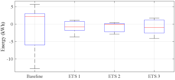
In this figure, the maximum and the minimum grid loads are illustrated by the whisker horizontal bars. The figure depicts the ETSs reduce the positive peak grid energy demand and the peak reverse power flow to the grid (negative grid load) that occurs due to excess PV power during the day in the baseline. Out of the three ETSs, the ETS 2 results in the lowest peak positive and negative grid energy loads as the users $\mathcal{P}$ predominantly exchange all their energy transactions with the CES system.

Fig. 8 shows the temporal variations of the CES energy charge levels with the three ETSs.

Additionally, Figs. 9(a), 9(b) and 9(c) depict the different energy transactions in the three ETSs.

Fig. 8 shows, in all systems, the CES system is charging during the day ($e_{s}(t)>0$) and discharging in the afternoon ($e_{s}(t)<0$). As shown in Figs. 9(a) and 9(b), in the ETSs 1 and 2, the CES system exchanges energy with both the users $\mathcal{P}$ and the grid, i.e., the profiles of $\sum_{n\in\mathcal{P}}y_{n}(t)$ and $e_{g}(t)$ have non-zero values. In these two systems, the CES charges during the day mainly due to the PV energy sold by the users ($\sum_{n\in\mathcal{P}}y_{n}(t)>0$). However, in ETS 3, because the users do not exchange energy with the CES, i.e., $\sum_{n\in\mathcal{P}}y_{n}(t)=0$, the CES charge-discharge profile $e_{s}(t)$ coincides with the CES provider’s grid energy trading profile $e_{g}(t)$ as shown in Fig. 9(c). Therefore, in the ETS 3, the charging of the CES during the day occurs mainly due to the energy bought by the CES provider ($e_{g}(t)>0$). In all three systems, the CES system discharges in the afternoon and that reduces the afternoon peak grid energy demand as shown in Fig. 6.

Fig. 10 compares the total revenue ($-f_{\text{cost}}$ in (11)) and the DN energy loss, by using (12), in the three ETSs with those of the baseline system.

As shown, all three ETSs are capable of reducing the DN energy loss of the baseline system by nearly 85%. Additionally, the total revenues of the three ETSs are higher than that in the baseline system. The total revenue decreases from the ETS 3 through the ETS 1 to the ETS 2. A similar trend was observed for the DN energy loss. In the ETS 3, both participating users and the CES provider receive positive cumulative revenues and that leads to the greatest revenue of the three systems. On the other hand, in the ETS 2, the users receive zero revenue because they trade energy only with the CES system ($l_{n}(t)=0$), without receiving a price for their energy transactions. That leads to the least revenue in the ETS 2. However, the reduction of the revenue of the ETS 2 compared to the revenue of the ETS 3, where the users only exchange energy with the grid, is only by 19%, and the reduction of the revenue of the ETS 1, where the users trade energy with both the grid and the CES system, compared to revenue of the ETS 3 is only by 7%. These trends highlight that energy trading between the users and the CES system can give a better trade-off between the DN power loss and energy cost reductions.

Fig. 11 illustrates the bus voltages of the baseline system.

As shown, due to excess PV power generation during the day, all buses of the feeder experience over-voltage conditions and in the afternoon, due to peak energy demand, the lower voltage limit is breached at buses 3-7. Figs. 12, 13 and 14 depict that, by exploiting the CES system charging-discharging with PV power generation, all three ETSs can regulate the voltage excursions in the DN that occurs in the baseline system.

We have studied the extent to which the integration of residential photovoltaic (PV) power with a community energy storage (CES) system can minimize distribution network (DN) power loss and energy costs, by comparing three different energy trading systems (ETSs). A network-constrained multi-objective optimization framework has been developed to study the trade-offs between the energy cost and DN power loss reductions while satisfying the DN voltage and current flow limits. Numerical results highlighted that energy trading between the PV users and the CES system can create a better trade-off between the network power loss and energy cost reductions while reducing peak electricity demand on the grid. Future work includes exploring methods for optimal sizing and location of the CES system and combining the ETS operations with behind-the-meter energy storage systems.

References

- [1] M. Baran and F. F. Wu, “Optimal sizing of capacitors placed on a radial distribution system,” IEEE Trans. Power Del., vol. 4, no. 1, pp. 735–743, Jan 1989.
- [2] J. von Appen, T. Stetz, M. Braun, and A. Schmiegel, “Local voltage control strategies for pv storage systems in distribution grids,” IEEE Trans. Smart Grid, vol. 5, no. 2, pp. 1002–1009, 2014.
- [3] M. Zeraati, M. E. Hamedani Golshan, and J. M. Guerrero, “Distributed control of battery energy storage systems for voltage regulation in distribution networks with high pv penetration,” IEEE Trans. Smart Grid, vol. 9, no. 4, pp. 3582–3593, July 2018.
- [4] S. Hashemi and J. Østergaard, “Efficient control of energy storage for increasing the pv hosting capacity of lv grids,” IEEE Trans. Smart Grid, vol. 9, no. 3, pp. 2295–2303, May 2018.
- [5] Z. Wang, C. Gu, F. Li, P. Bale, and H. Sun, “Active demand response using shared energy storage for household energy management,” IEEE Trans. Smart Grid, vol. 4, no. 4, pp. 1888–1897, Dec 2013.
- [6] B. Celik, R. Roche, D. Bouquain, and A. Miraoui, “Decentralized neighborhood energy management with coordinated smart home energy sharing,” IEEE Trans. Smart Grid, vol. 9, no. 6, pp. 6387–6397, Nov 2018.
- [7] T. Jiang, Y. Cao, L. Yu, and Z. Wang, “Load shaping strategy based on energy storage and dynamic pricing in smart grid,” IEEE Trans. Smart Grid, vol. 5, no. 6, pp. 2868–2876, Nov 2014.
- [8] J. Tant, F. Geth, D. Six, P. Tant, and J. Driesen, “Multiobjective battery storage to improve pv integration in residential distribution grids,” IEEE Trans. Sustain. Energy, vol. 4, no. 1, pp. 182–191, Jan 2013.
- [9] W. Shi, X. Xie, C. Chu, and R. Gadh, “Distributed optimal energy management in microgrids,” IEEE Trans. Smart Grid, vol. 6, no. 3, pp. 1137–1146, May 2015.
- [10] N. Karthikeyan, J. R. Pillai, B. Bak-Jensen, and J. W. Simpson-Porco, “Predictive control of flexible resources for demand response in active distribution networks,” IEEE Trans. Power Syst., vol. 34, no. 4, pp. 2957–2969, July 2019.
- [11] H. Gao, L. Wang, J. Liu, and Z. Wei, “Integrated day-ahead scheduling considering active management in future smart distribution system,” IEEE Trans. Power Syst., vol. 33, no. 6, pp. 6049–6061, Nov 2018.
- [12] M. Nick, R. Cherkaoui, and M. Paolone, “Optimal allocation of dispersed energy storage systems in active distribution networks for energy balance and grid support,” IEEE Trans. Power Syst., vol. 29, no. 5, pp. 2300–2310, Sep. 2014.
- [13] C. P. Mediwaththe and L. Blackhall, “Network-aware demand-side management framework with a community energy storage system considering voltage constraints,” IEEE Trans. Power Syst., pp. 1–1, 2020.
- [14] W. Lin and E. Bitar, “Decentralized stochastic control of distributed energy resources,” IEEE Trans. Power Syst., vol. 33, no. 1, pp. 888–900, Jan 2018.
- [15] O. Grodzevich and O. Romanko, “Normalization and other topics in multi-objective optimization,” in Fields MITACS Ind. Prob. Workshop, Aug 2006.
- [16] T. L. Saaty, “Decision making — the analytic hierarchy and network processes (AHP/ANP),” J. Syst. Sci. Syst. Eng., vol. 13, no. 1, pp. 1–35, Mar 2004.
- [17] S. Boyd and L. Vandenberghe, Convex Optimization, 1st ed. Cambridge University Press, 2004, pp. 67–95.
- [18] M. Shaw, B. Sturmberg, L. Guo, X. Gao, E. Ratnam, and L. Blackhall, “The Nextgen Energy Storage Trial in the ACT, Australia,” in Proc. ACM Conf. on Future Energy Syst., 2019, pp. 439–442.
- [19] Origin, “VIC residential energy price fact sheet,” 2018. [Online]. Available: https://bit.ly/2UEWqzm